Spin-excitations of the quantum Hall ferromagnet of composite fermions

Abstract

The spin-excitations of a fractional quantum Hall system are evaluated within a bosonization approach. In a first step, we generalize Murthy and Shankar’s Hamiltonian theory of the fractional quantum Hall effect to the case of composite fermions with an extra discrete degree of freedom. Here, we mainly investigate the spin degrees of freedom, but the proposed formalism may be useful also in the study of bilayer quantum-Hall systems, where the layer index may formally be treated as an isospin. In a second step, we apply a bosonization scheme, recently developed for the study of the two-dimensional electron gas, to the interacting composite-fermion Hamiltonian. The dispersion of the bosons, which represent quasiparticle-quasihole excitations, is analytically evaluated for fractional quantum Hall systems at $\nu=1/3$ and $\nu=1/5$. The finite width of the two-dimensional electron gas is also taken into account explicitly. Furthermore, we consider the interacting bosonic model and calculate the lowest-energy state for two bosons. In addition to a continuum describing scattering states, we find a bound-state of two bosons. This state is interpreted as a pair excitation, which consists of a skyrmion of composite fermions and an antiskyrmion of composite fermions. The dispersion relation of the two-boson state is evaluated for $\nu=1/3$ and $\nu=1/5$. Finally, we show that our theory provides the microscopic basis for a phenomenological non-linear sigma-model for studying the skyrmion of composite fermions.

I Introduction

Quantum Hall physics – the study of two-dimensional (2D) electrons in a strong magnetic field – has revealed a lot of unexpected phenomena during the last 25 years.perspectives Apart from the integer and fractional quantum Hall effects (IQHE and FQHE, respectively), which have been identified as macroscopic quantum phenomena, exotic topological spin excitations are displayed by these systems. The physical properties of quantum Hall systems are governed by the Landau quantization; the energy of 2D electrons with a band mass $m_{B}$ and charge $-e$ in a perpendicular magnetic field $B$ is quantized into equidistant energy levels, the so-called Landau levels (LLs), with a level separation $\hbar w_{C}=\hbar eB/m_{B}c$. The large LL degeneracy is characterized by the flux density $n_{\phi}=1/2\pi l_{B}^{2}$, given in terms of the magnetic length $l_{B}=\sqrt{\hbar c/eB}$, and the LL filling is thus defined as the ratio $\nu=n_{el}/n_{\phi}$ of the electronic density $n_{el}$ and $n_{\phi}$. Due to the Zeeman effect, each LL $n$ is split into two spin-branches with an energy separation $g^{*}\mu_{B}B$, where $g^{*}$ is the effective Landé factor ($g^{*}=-0.44$ for GaAs), and $\mu_{B}=2\hbar e/m$ is the Bohr magneton. Because the band mass is reduced with respect to the bare electron mass $m$ ($m_{B}=0.068m$ for GaAs), the spin-branch separation is about $70$ times smaller than the LL separation.

The IQHE may be understood in a one-particle picture, in which the Coulomb interaction is only a small perturbation. If $\nu=N$, with integral $N$, the ground state is non-degenerate and one has to provide a finite energy to promote an electron to the next higher level. Due to the localization of additional electrons by residual impurities in the sample, the Hall resistance remains at its quantized value $R_{H}=h/e^{2}N$ over a certain range of the magnetic field. This plateau in the Hall resistance is accompanied by a vanishing longitudinal resistance, and both are the signature of the quantum Hall effect. If the lower spin branch of the $n$-th LL is completely filled, one has $N=2n+1$, and $N=2n+2$ in the case of complete filling of both spin branches.

The one-particle picture ceases to be valid at partial filling $\nu\neq N$, where one is confronted with the LL degeneracy. In this limit, electrons in a partially filled level are strongly correlated due to their mutual Coulomb repulsion, which constitutes the relevant energy scale. In the lowest LL, the formation of composite fermions (CFs) leads to incompressible quantum liquids at $\nu=p/(2sp+1)$.jain ; heinonen The FQHE, displayed by these liquids, may be interpreted as an IQHE of CFs. The physical properties of CFs have been extensively studied in the framework of Jain’s wave-function approach,jain ; heinonen which is a generalization of Laughlin’s trial wave functions.laughlin A complementary field-theoretical formalism, based on Chern-Simons transformations, has been proposed by Lopez and Fradkin.lopezfradkin The latter has been particularly successful in the description of the metallic state at $\nu=1/2$, which may be interpreted as a Fermi sea of CFs.HLR More recently, Murthy and Shankar have developed a Hamiltonian theory of the FQHE, a second-quantized approach.MS It systematically accounts for the mechanism of how these excitations are formed and what are their constituents, namely, electrons or holes bound to an even number of vortex-like objects.

Although the main features of the IQHE may be understood in the framework of a noninteracting model of spin-polarized electrons, the study of spin-excitations at $\nu=1$, when only one spin-branch of the lowest LL ($n=0$) is completely filled, requires a more complete treatment of the problem. Indeed, the lowest-energy excitations involve a spin reversal, and the spin degree of freedom must be considered explicitly. In addition to spin-wave excitations, which are gapped due to the Zeeman effect, one finds topological skyrmion excitations;skyrme if the Coulomb interaction is large with respect to the Zeeman gap, it is energetically favorable to distribute the spin reversal over a group of neighboring spins.leekane ; sondhi ; moon These skyrmion excitations give rise to unusual spin polarizations.barrett More recently, the different spin excitations at $\nu=1$ have been investigated in a bosonization approach.doretto Although the bosonization method of fermionic systems is well established for one-dimensional electron systems,delf ; voit only few generalizations to higher dimensions have been proposed. castroneto ; houghton One particular example is a recently developed bosonization scheme for the 2D electron gas (2DEG) in a magnetic field.harry ; doretto The extension presented in Ref. doretto, , in particular, allows for the treatment of complex many-body structures, such as small skyrmion-antiskyrmion pairs in terms of bound states of the bosonic excitations.

Here, we generalize the Hamiltonian theory of the FQHE of Ref. MS, to incorporate spin or any other discrete degree of freedom. Although in this paper we apply our theory to the investigation of spin excitations, the developed formalism has a wider range of application and may also be useful for further studies on bilayer quantum Hall systems, for which the layer index is formally treated as an isospin.perspectives ; moon For certain values of the magnetic field, the ground state may be viewed as a $\nu=1$ state of CFs, and it is therefore natural to test the bosonization scheme for these cases. The method allows us to investigate the CF excitation spectrum and to describe, for example, skyrmion-like excitations at filling factors such as $\nu=1/3$. Indeed, optically pumped nuclear magnetic resonance measurements, which give information about the spin polarization of the 2DEG, indicate the existence of such excitation around $\nu=1/3$.khandelwal2

The outline of the paper is the following. The generalization of the Hamiltonian theory to the case of fermions with an extra discrete degree of freedom is presented in Sec. II. In Sec. III, we apply the previously developed bosonization method doretto to the obtained CF Hamiltonian and study the dispersion relation of the resulting bosons. Bound states of two of these elementary excitations, which we interpret as small skyrmion-antiskyrmion pairs, are also considered. Sec. IV is devoted to the semiclassical limit of our approach, from which we show that an effective Lagrangian, similar to the one suggested by Sondhi et al.,sondhi accounts for the long-wavelength properties of the system. A summary of the main results is finally presented in Sec. V.

II Hamiltonian Theory of CFs with Spin

Our first aim is to derive the Hamiltonian theory for electrons with spin in the lowest LL and construct the CF basis. In principle, the generalization of the algebraic properties of the Murthy and Shankar model [Ref. MS, ] to the case of discrete degrees of freedom, such as the spin or the isospin in the context of bilayer quantum Hall systems, may be written down intuitively. In this section, however, they are derived, with the help of a set of transformations, from the microscopic model of an interacting 2DEG, with spin $\sigma=\uparrow$ (+1) or $\downarrow$ (-1) in a perpendicular magnetic field $B{\bf e}_{z}=\mbox{\boldmath$\nabla$}\times{\bf A}$. The Hamiltonian of the system reads, in terms of the electron fields $\psi_{\sigma}({\bf r})$ and $\psi_{\sigma}^{\dagger}({\bf r})$ ($\hbar=c=1$)

$$\hat{H}=\hat{H}_{0}+\hat{H}_{Z}+\hat{H}_{I},$$ (1)

where the orbital part is

$$\hat{H}_{0}=\frac{1}{2m_{B}}\sum_{\sigma}\int d^{2}r\psi_{\sigma}^{\dagger}({\bf r})\left[-i\mathbf{\mbox{\boldmath$\nabla$}}+e{\bf A}({\bf r})\right]^{2}\psi_{\sigma}({\bf r}),$$ (2)

the Zeeman term is

$$\hat{H}_{Z}=\frac{1}{2}g^{*}\mu_{B}B\sum_{\sigma}\sigma\int d^{2}r\psi_{\sigma}^{\dagger}({\bf r})\psi_{\sigma}({\bf r}),$$ (3)

and the interaction Hamiltonian is

$$\hat{H}_{I}=\frac{1}{2}\sum_{\sigma,\sigma^{\prime}}\int d^{2}rd^{2}r^{\prime}\psi_{\sigma}^{\dagger}({\bf r})\psi_{\sigma^{\prime}}^{\dagger}({\bf r}^{\prime})V({\bf r}-{\bf r}^{\prime})\psi_{\sigma^{\prime}}({\bf r}^{\prime})\psi_{\sigma}({\bf r}),$$ (4)

which couples electrons with different spin orientation. Here, $V({\bf r})=e^{2}/\epsilon r$ is the isotropic Coulomb interaction potential, with $r=|{\bf r}|$, and $\epsilon$ is the dielectric constant of the host semiconductor.

II.1 Microscopic Theory

Following closely the steps of Ref. MS, , we perform a Chern-Simons transformation on the electron fields, defined by

$$\psi_{\sigma}({\bf r})=e^{-2is_{\sigma}\int d^{2}r^{\prime}\theta({\bf r}-{\bf r}^{\prime})\rho_{\sigma}({\bf r}^{\prime})}\psi_{\sigma}^{CS}({\bf r}),$$ (5)

where $\theta({\bf r})$ is the angle between the vector ${\bf r}$ and the $x$-axis. The density operator reads $\rho_{\sigma}({\bf r})=\psi_{\sigma}^{\dagger}({\bf r})\psi_{\sigma}({\bf r})=\psi_{\sigma}^{CS\dagger}({\bf r})\psi_{\sigma}^{CS}({\bf r})$. Thus, the Zeeman $\hat{H}_{Z}$ and the interaction $\hat{H}_{I}$ terms in Eq. (1) remain invariant under the above transformation. In order to describe fermionic fields, which is the case of interest here, $s_{\sigma}$ must be integer. Note that this transformation breaks the $SU(2)$ symmetry explicitly unless $s_{\uparrow}=s_{\downarrow}$. For the symmetric case, a Hamiltonian theory for bilayer systems has very recently been established by Stanić and Milovanović who investigated composite bosons at a total filling factor $\nu=1$.stanic Here, we discuss the more general case in which the electronic density of $\uparrow$-electrons is not necessarily the same as that of $\downarrow$-electrons. The transformation generates the two-component spinor Chern-Simons vector potential ${\bf a}_{\sigma}^{CS}({\bf r})$ with

$$\mbox{\boldmath$\nabla$}\times{\bf a}_{\sigma}^{CS}({\bf r})=-2s_{\sigma}\phi_{0}\rho_{\sigma}({\bf r}){\bf e}_{z},$$ (6)

in terms of the flux quantum $\phi_{0}=2\pi/e$.

In order to decouple the electronic degrees of freedom and the complicated fluctuations of the Chern-Simons field, Murthy and Shankar introduced an auxiliary vector potentialMS ${\bf a}_{\sigma}({\bf q})$, which was inspired by the plasmon description proposed by Bohm and Pines for the electron gas.bohm If the spin degree of freedom is taken into account, this vector potential consists of two spinor components, both of which are chosen transverse to satisfy the Coulomb gauge, $\mbox{\boldmath$\nabla$}\cdot{\bf a}_{\sigma}({\bf r})=0$. For its Fourier components one thus finds ${\bf a}_{\sigma}({\bf q})=-i{\bf e}_{z}\times{\bf e}_{q}a_{\sigma}({\bf q})$, where ${\bf e}_{q}={\bf q}/|{\bf q}|$ is the unit vector in the direction of propagation of the field. Its conjugate field is chosen longitudinal, ${\bf P}_{\sigma}({\bf q})=i{\bf e}_{q}P_{\sigma}({\bf q})$, with the commutation relations

$$\left[a_{\sigma}({\bf q}),P_{\sigma^{\prime}}(-{\bf q}^{\prime})\right]=i\delta_{\sigma,\sigma^{\prime}}\delta_{{\bf q},{\bf q}^{\prime}}.$$ (7)

The Hilbert space is enlarged by these non-physical degrees of freedom, and one therefore has to impose the constraint $a_{\sigma}({\bf q})|\phi\rangle=0$ on the physical states $|\phi\rangle$. The orbital part (2) of the Hamiltonian thus becomes

$$\hat{H}_{0}^{CS} = \frac{1}{2m_{B}}\sum_{\sigma}\int d^{2}r\psi_{\sigma}^{CS\dagger}({\bf r})$$ (8)

$$\times\left[\mbox{\boldmath$\Pi$}_{\sigma}+e:{\bf a}_{\sigma}^{CS}({\bf r}):+e{\bf a}_{\sigma}({\bf r})\right]^{2}\psi_{\sigma}^{CS}({\bf r}),$$

where the mean-field part of the Chern-Simons vector potential $\langle{\bf a}_{\sigma}^{CS}({\bf r})\rangle$ has been absorbed into a generalized momentum $\mbox{\boldmath$\Pi$}_{\sigma}=-i\mbox{\boldmath$\nabla$}+e\left[{\bf A}({\bf r})+\langle{\bf a}_{\sigma}^{CS}({\bf r})\rangle\right]$, and $:{\bf a}_{\sigma}^{CS}({\bf r}):$ denotes its normal-ordered fluctuations. The conjugate field $P_{\sigma}({\bf q})$ generates the translations of the vector potential, and one may therefore choose the unitary transformation $\psi_{\sigma}^{CS}({\bf r})=U_{\sigma}\psi_{\sigma}^{CP}({\bf r})$, in terms of the composite-particle field $\psi_{\sigma}^{CP}({\bf r})$, with

$$U_{\sigma}=\exp\left(i\sum_{{\bf q}}^{Q}P_{\sigma}(-{\bf q})\frac{4\pi s_{\sigma}}{q}\delta\rho({\bf q})\right),$$

to make the long-range ($q<Q$) fluctuations of the Chern-Simons vector potential vanish. The transformed Hamiltonian (8) without the short-range terms related to $:a_{\sigma}^{CS}({\bf q}):$ thus reads

$$\hat{H}_{0}^{CP}=\sum_{\sigma}\int d^{2}r\psi_{\sigma}^{CP\dagger}({\bf r})\mathcal{H}_{\sigma}({\bf r})\psi_{\sigma}^{CP}({\bf r}),$$ (9)

with the Hamiltonian density

$$\mathcal{H}_{\sigma} = \frac{\mbox{\boldmath$\Pi$}_{\sigma}^{2}}{2m_{B}}+\frac{1}{2m_{B}}\left[{\bf a}_{\sigma}({\bf r})+4\pi s_{\sigma}{\bf P}_{\sigma}({\bf r})\right]^{2}$$ (10)

$$+\frac{1}{m_{B}}\mbox{\boldmath$\Pi$}_{\sigma}\cdot\left[{\bf a}_{\sigma}({\bf r})+4\pi s_{\sigma}{\bf P}_{\sigma}({\bf r})\right].$$

The second term is the Hamiltonian density of a quantum mechanical harmonic oscillator, as may be seen from the commutation relations (7). In the absence of the third term of Eq. (10), which couples the electric current density and the harmonic oscillators, one may write down the field as a product of the ground-state wavefunction of the oscillators $\chi({\bf r})$ and $\phi^{*}({\bf r})$, where $\phi^{*}({\bf r})$ is the $N$-particle wavefunction of charged particles in an effective magnetic field

$$\mbox{\boldmath$\nabla$}\times\left[{\bf A}({\bf r})+\langle{\bf a}_{\sigma}^{CS}({\bf r})\rangle\right]=B_{\sigma}^{*}{\bf e}_{z},$$

with $B_{\sigma}^{*}=B-2s_{\sigma}\phi_{0}n_{el}^{\sigma}=B_{\sigma}/(2s_{\sigma}p_{\sigma}+1)$, in terms of the average density $n_{el}^{\sigma}$ of electrons with spin $\sigma$. In the absence of correlations between electrons with different spin, the filling of each spin branch may thus be characterized by a renormalized filling factor, $\nu_{\sigma}^{*}=n_{el}^{\sigma}2\pi l_{\sigma}^{*2}$, with the new magnetic length $l_{\sigma}^{*}=1/\sqrt{eB_{\sigma}^{*}}$. The oscillator wavefunction becomes, with the help of the transformed constraint, $\left[qa_{\sigma}({\bf q})-4\pi s_{\sigma}\rho_{\sigma}({\bf q})\right]|\phi\rangle=0$

$$\chi({\bf r})=\exp\left[-\sum_{\sigma,{\bf q}}2\pi s_{\sigma}\delta\rho_{\sigma}(-{\bf q})\frac{1}{q^{2}}\delta\rho_{\sigma}({\bf q})\right].$$

The exponent may be rewritten in terms of the complex coordinates $z_{j}=x_{j}+iy_{j}$ for spin-up and $w_{\mu}=x_{\mu}+iy_{\mu}$ for spin-down particles kane

$$\sum_{\sigma,{\bf q}}2\pi s_{\sigma}\delta\rho_{\sigma}(-{\bf q})\frac{1}{q^{2}}\delta\rho_{\sigma}({\bf q})\simeq$$

$$\sum_{i<j}2s_{\uparrow}\ln|z_{i}-z_{j}|-\sum_{j}\frac{|z_{j}|^{2}}{4l_{B}^{2}}c_{\uparrow}^{2}+$$

$$\sum_{\mu<\nu}2s_{\downarrow}\ln|w_{\mu}-w_{\nu}|-\sum_{j}\frac{|w_{\mu|^{2}}}{4l_{B}^{2}}c_{\downarrow}^{2},$$

where $c_{\sigma}^{2}=2s_{\sigma}p_{\sigma}/(2s_{\sigma}p_{\sigma}+1)$, at integer values of $\nu_{\sigma}^{*}=p_{\sigma}$. The complete wavefunction therefore becomes

$$\psi(z_{i},w_{\mu})=\prod_{i<j}\left(z_{i}-z_{j}\right)^{2s_{\uparrow}}\prod_{\mu<\nu}\left(w_{\mu}-w_{\nu}\right)^{2s_{\downarrow}}\phi^{*}(z_{i},w_{\mu}),$$ (11)

where the Gaussian factors have been absorbed into the electronic part of the wavefunction $\phi^{*}(z_{i},w_{\mu})$. If there are no correlations between particles with different spin orientation, i.e. in the absence of interactions, the electronic part of the wavefunction may be written as a product, $\phi^{*}(z_{i},w_{\mu})=\phi_{p_{\uparrow}}^{\uparrow}(z_{i})\phi_{p_{\downarrow}}^{\downarrow}(w_{\mu})$, and Eq. (11) thus represents a product of two Laughlin wavefunctionslaughlin (for $p_{\sigma}=1$) or unprojected Jain wavefunctionsjain (for $p_{\sigma}>1$) for the two spin orientations. If one includes correlations between particles with different spin orientation, one may use the ansatz

$$\phi^{*}(z_{i},w_{\mu})=\phi_{p_{\uparrow}}^{\uparrow}(z_{i})\phi_{p_{\downarrow}}^{\downarrow}(w_{\mu})\prod_{i,\mu}\left(z_{i}-w_{\mu}\right)^{m},$$

with integral $m$. For $p_{\sigma}=1$, one recovers Halperin’s wavefunctions, halperin3 if

$$\phi_{1}^{\uparrow}(z_{i})=\prod_{i<j}(z_{i}-z_{j})~{}e^{-\sum_{j}|z_{j}|^{2}/4l_{B}^{2}},$$

and similarly

$$\phi_{1}^{\downarrow}(w_{\mu})=\prod_{\mu<\nu}(w_{\mu}-w_{\nu})~{}e^{-\sum_{\nu}|w_{\nu}|^{2}/4l_{B}^{2}}.$$

In this case the filling factors of the two spin branches become $\nu_{\sigma}=(2s_{\sigma}-m)/(s_{\uparrow}s_{\downarrow}-m^{2})$. For larger values of $p_{\sigma}$, the wavefunction (11) contains components in higher LLs and is thus no longer analytic, as required by the lowest LL condition. jach Eq. (11) must therefore be projected into the lowest LL, and the final trial wavefunctions become

$$\psi(z_{i},w_{\mu}) = \mathcal{P}\prod_{i<j}\left(z_{i}-z_{j}\right)^{2s_{\uparrow}}\prod_{\mu<\nu}\left(w_{\mu}-w_{\nu}\right)^{2s_{\downarrow}}$$ (12)

$$\times\prod_{i,\mu}\left(z_{i}-w_{\mu}\right)^{m}\phi_{p_{\uparrow}}^{\uparrow}(z_{i})\phi_{p_{\downarrow}}^{\downarrow}(w_{\mu}),$$

where $\mathcal{P}$ denotes the projection to the lowest LL. They may be interpreted as a CF generalization of Halperin’s wavefunctions.halperin3

Up to this point, the coupling term between the electronic and oscillator degrees of freedom in the Hamiltonian density (10) has been neglected. Murthy and Shankar have proposed a decoupling procedure, which also applies to the case of electrons with spin, with the only difference that two unitary transformations $\bar{U}_{\sigma}$ are required for the two spin orientations. The reader is referred to their review (Ref. MS, ) for the details of the decoupling transformations, and we will limit ourselves to the presentation of the results. With the choice of equal number of oscillators and particles for each spin orientation, the kinetic term in the Hamiltonian vanishes, and the model in the limit of small wave vectors becomes

$$\hat{H} = \sum_{\sigma,{\bf q}}\omega_{C}A_{\sigma}^{\dagger}({\bf q})A_{\sigma}({\bf q})+\frac{1}{2}\gamma\sum_{\sigma}\sigma\rho_{\sigma}({\bf q}=0)$$ (13)

$$+\frac{1}{2}\sum_{{\bf q}}\sum_{\sigma,\sigma^{\prime}}v_{0}(q)\rho_{\sigma}(-{\bf q})\rho_{\sigma^{\prime}}({\bf q})$$

where $A_{\sigma}({\bf q})\equiv\left[a_{\sigma}({\bf q})+4\pi is_{\sigma}P_{\sigma}({\bf q})\right]/\sqrt{8\pi s_{\sigma}}$, $\gamma=g^{*}\mu_{B}B$ is the Zeeman energy, and

$$v_{0}=\frac{2\pi e^{2}}{\epsilon q}e^{-|ql_{B}|^{2}/2}$$ (14)

is the interaction potential in the lowest LL. The transformed density operators may be expressed in first quantization with the help of the position of the $j$-th particle ${\bf r}_{j}$ and its generalized momentum $\mbox{\boldmath$\Pi$}_{\sigma}^{j}$,

$$\rho_{\sigma}({\bf q})=\sum_{j}e^{-i{\bf q}\cdot{\bf r}_{j}}\left[1-\frac{il_{B}^{2}}{(1+c_{\sigma})}{\bf q}\times\mbox{\boldmath$\Pi$}_{\sigma}^{j}+\mathcal{O}(q^{2})\right],$$ (15)

where terms of order $\mathcal{O}(q^{2})$ have been omitted, and the oscillators are chosen to remain in their ground state, $\langle A_{\sigma}({\bf q})\rangle=\langle A_{\sigma}^{\dagger}({\bf q})\rangle=0$. The transformed constraint is given by

$$\chi_{\sigma}({\bf q})|\phi\rangle=0,$$ (16)

with

$$\chi_{\sigma}({\bf q})=\sum_{j}e^{-i{\bf q}\cdot{\bf r}_{j}}\left[1+il_{B}^{2}\frac{{\bf q}\times\mbox{\boldmath$\Pi$}_{\sigma}^{j}}{c_{\sigma}(1+c_{\sigma})}+\mathcal{O}(q^{2})\right].$$ (17)

To construct the theory at larger wave vectors, Shankar had the ingenious insight that if one considers the terms in the expressions (15) and (17) as the first terms of a series expansion of an exponential,

$$\bar{\rho}_{\sigma}({\bf q})=\sum_{j}e^{-i{\bf q}\cdot{\bf R}_{\sigma,j}^{(e)}}\qquad{\rm and}\qquad\bar{\chi}_{\sigma}({\bf q})=\sum_{j}e^{-i{\bf q}\cdot{\bf R}_{\sigma,j}^{(v)}},$$

both operators find a compelling physical interpretation.shankar The operator

$${\bf R}_{\sigma}^{(e)}={\bf r}-\frac{l_{B}^{2}}{(1+c_{\sigma})}{\bf e}_{z}\times\mbox{\boldmath$\Pi$}_{\sigma}$$

may be interpreted as the electronic guiding center operator, and its components satisfy the correct commutation relations, $\left[X_{\sigma}^{(e)},Y_{\sigma^{\prime}}^{(e)}\right]=-il_{B}^{2}\delta_{\sigma,\sigma^{\prime}}$, where the number index has been omitted. This leads to the algebra for the Fourier components of the density in the lowest LL GMP

$$\left[\bar{\rho}_{\sigma}({\bf q}),\bar{\rho}_{\sigma^{\prime}}({\bf q}^{\prime})\right]=\delta_{\sigma,\sigma^{\prime}}2i\sin\left(\frac{{\bf q}\wedge{\bf q}^{\prime}l_{B}^{2}}{2}\right)\bar{\rho}_{\sigma}({\bf q}+{\bf q}^{\prime}),$$ (18)

where we have defined ${\bf q}\wedge{\bf q}^{\prime}=({\bf q}\times{\bf q}^{\prime})_{z}$. In the same manner, the components of the operator

$${\bf R}_{\sigma}^{(v)}={\bf r}+\frac{l_{B}^{2}}{c_{\sigma}(1+c_{\sigma})}{\bf e}_{z}\times\mbox{\boldmath$\Pi$}_{\sigma}$$

satisfy $\left[X_{\sigma}^{(v)},Y_{\sigma^{\prime}}^{(v)}\right]=il_{B}^{2}\delta_{\sigma,\sigma^{\prime}}/c_{\sigma}^{2}$, which leads to

$$\left[\bar{\chi}_{\sigma}({\bf q}),\bar{\chi}_{\sigma^{\prime}}({\bf q}^{\prime})\right]=-\delta_{\sigma,\sigma^{\prime}}2i\sin\left(\frac{{\bf q}\wedge{\bf q}^{\prime}l_{B}^{2}}{2c_{\sigma}^{2}}\right)\bar{\chi}_{\sigma}({\bf q}+{\bf q}^{\prime}).$$ (19)

The operator $\bar{\chi}_{\sigma}({\bf q})$, which characterizes the constraint, may thus be interpreted as the density operator of a second type of particle with charge $-c_{\sigma}^{2}$, in units of the electronic charge. However, this particle, the so-called pseudo-vortex, only exists in the enlarged Hilbert space because it is an excitation of the correlated electron liquid and must be described in terms of the electronic degrees of freedom. A similar algebra has been investigated by Pasquier and Haldane in the description of bosons at $\nu=1$.PH The final model Hamiltonian thus reads

$$\hat{H} = \frac{1}{2}\gamma\sum_{\sigma}\sigma\bar{\rho}_{\sigma}({\bf q}=0)$$ (20)

$$+\frac{1}{2}\sum_{{\bf q}}\sum_{\sigma,\sigma^{\prime}}v_{0}(q)\bar{\rho}_{\sigma}(-{\bf q})\bar{\rho}_{\sigma^{\prime}}({\bf q})$$

with the constraint (16) and the algebras (18) and (19) for the electronic and the pseudo-vortex density, respectively. In the case of bilayer systems, the interaction between particles in the same layer is different (stronger) than that between particles in the different layers. This breaks the $SU(2)$ symmetry, and one thus has to replace $v_{0}(q)\rightarrow v_{0}^{\sigma,\sigma^{\prime}}(q)$.moon

II.2 Model in the CF-Basis

In order to construct the CF representation of the model, Murthy and Shankar proposed the “preferred” combination of electronic and pseudo-vortex density,MS ; shankar

$$\bar{\rho}_{\sigma}^{P}({\bf q})=\bar{\rho}_{\sigma}({\bf q})-c_{\sigma}^{2}\bar{\chi}_{\sigma}({\bf q}),$$ (21)

which plays the role of the CF density. This approximation allows one to omit the constraint in the case of a gapped ground state,MS whereas it fails in the limit $\nu=1/2$, where the system becomes compressibleHLR and where the constraint has to be taken into account explicitly in a conserving approximation.approxcons The CF basis is introduced after a variable transformation of the guiding-center coordinates ${\bf R}_{\sigma}^{(e)}$ and ${\bf R}_{\sigma}^{(v)}$,

$${\bf R}_{\sigma}^{(e)}={\bf R}_{\sigma}+\mbox{\boldmath$\eta$}_{\sigma}c_{\sigma}\qquad{\bf R}_{\sigma}^{(v)}={\bf R}_{\sigma}+\mbox{\boldmath$\eta$}_{\sigma}/c_{\sigma}.$$

The new variables play the role of the CF guiding center (${\bf R}_{\sigma}$) and the CF cyclotron variable ($\mbox{\boldmath$\eta$}_{\sigma}$) and commute with each other. Their components, however, satisfy the commutation relations

$$\left[X_{\sigma},Y_{\sigma^{\prime}}\right]=-i\delta_{\sigma,\sigma^{\prime}}l_{\sigma}^{*2},\qquad\left[\eta_{\sigma}^{x},\eta_{\sigma^{\prime}}^{y}\right]=i\delta_{\sigma,\sigma^{\prime}}l_{\sigma}^{*2},$$

in terms of the CF magnetic length $l_{\sigma}^{*}=l_{B}/\sqrt{1-c_{\sigma}^{2}}$. The CF density operator therefore becomes

$$\bar{\rho}_{\sigma}^{P}({\bf q})=\sum_{n,n^{\prime};m,m^{\prime}}G_{m,m^{\prime}}(ql_{\sigma}^{*})F_{n,n^{\prime}}(q)c_{n,m;\sigma}^{\dagger}c_{n^{\prime},m^{\prime};\sigma},$$ (22)

where $c_{n,m;\sigma}^{\dagger}$ creates a CF with spin $\sigma$ in the state $|n,m\rangle$. The quantum number $n$ denotes the CF-LL, and $m$ indicates the CF guiding-center state. The matrix elements are given by MS ; goerbig04

$$G_{m,m^{\prime}}(ql_{\sigma}^{*}) = \sqrt{\frac{m^{\prime}!}{m!}}\left(\frac{-i(q_{x}+iq_{y})l_{\sigma}^{*}}{\sqrt{2}}\right)^{m-m^{\prime}}$$ (23)

$$\times L_{m^{\prime}}^{m-m^{\prime}}\left(\frac{q^{2}l_{\sigma}^{*2}}{2}\right)e^{-q^{2}l_{\sigma}^{*2}/4}$$

for $m\geq m^{\prime}$, and

$$F_{n,n^{\prime}}(q) = \sqrt{\frac{n^{\prime}!}{n!}}\left(\frac{-i(q_{x}-iq_{y})l_{\sigma}^{*}c_{\sigma}}{\sqrt{2}}\right)^{n-n^{\prime}}$$

$$\times e^{-q^{2}l_{\sigma}^{*2}c_{\sigma}^{2}/4}\left[L_{n^{\prime}}^{n-n^{\prime}}\left(\frac{q^{2}l_{\sigma}^{*2}c_{\sigma}^{2}}{2}\right)\right.$$

$$\left.-c_{\sigma}^{2(1-n+n^{\prime})}e^{-(ql_{B})^{2}/2c_{\sigma}^{2}}L_{n^{\prime}}^{n-n^{\prime}}\left(\frac{q^{2}l_{\sigma}^{*2}}{2c_{\sigma}^{2}}\right)\right]$$

for $n\geq n^{\prime}$.

We now restrict the Hilbert space to the lowest CF-LL. In this case, the CF density operator $\bar{\rho}^{P}_{\sigma}({\bf r})$ reads $\langle\bar{\rho}_{\sigma}^{P}({\bf q})\rangle_{n=0}=F_{n=0}^{CF}(q)\bar{\bar{\rho}}_{\sigma}({\bf q})$, where

$$F_{n=0}^{CF}(q)=F_{0,0}(q)=e^{-|ql^{*}c|^{2}/4}\left[1-c^{2}e^{-|ql_{B}|^{2}/2c^{2}}\right]$$ (25)

is the CF form factor, $p_{\uparrow}=p_{\downarrow}=1$, $s_{\uparrow}=s_{\downarrow}=s$, and therefore $c_{\uparrow}=c_{\downarrow}=c$ and $l^{*}_{\uparrow}=l^{*}_{\downarrow}=l^{*}$ (symmetric model). The electronic filling factor is thus given by $\nu=1/(2s+1)$, and the projected CF density operator is

$$\bar{\bar{\rho}}_{\sigma}({\bf q})=\sum_{m,m^{\prime}}G_{m,m^{\prime}}(ql^{*})c_{m,\sigma}^{\dagger}c_{m^{\prime},\sigma},$$ (26)

where $c_{m,\sigma}^{\dagger}$ creates a spin $\sigma$ composite fermion in the lowest CF-LL and where we have omitted the level index. The projected CF density operators satisfy a similar algebra as the projected electron density operators,GMP ; goerbig04

$$\left[\bar{\bar{\rho}}_{\sigma}({\bf q}),\bar{\bar{\rho}}_{\sigma^{\prime}}({\bf q}^{\prime})\right]=\delta_{\sigma,\sigma^{\prime}}2i\sin\left(\frac{{\bf q}\wedge{\bf q}^{\prime}l_{\sigma}^{*2}}{2}\right)\bar{\bar{\rho}}_{\sigma}({\bf q}+{\bf q}^{\prime}),$$ (27)

just with the magnetic length $l_{B}$ replaced by the CF magnetic length $l^{*}$. The Hamiltonian, which describes the low-energy excitations of the FQHE system at $\nu^{*}=1$ is thus given by

$$\hat{H} = \frac{1}{2}\gamma\sum_{\sigma}\sum_{m}\sigma c_{m,\sigma}^{\dagger}c_{m,\sigma}$$ (28)

$$+\frac{1}{2}\sum_{\sigma,\sigma^{\prime}}\sum_{{\bf q}}v_{0}(q)\left[F_{n=0}^{CF}(q)\right]^{2}\bar{\bar{\rho}}_{\sigma}(-{\bf q})\bar{\bar{\rho}}_{\sigma^{\prime}}({\bf q})$$

$$= \hat{H}_{Z}+\hat{H}_{I}$$

Note the similarity with the original Hamiltonian (20); the product $v_{0}(q)\left[F_{n=0}^{CF}(q)\right]^{2}$ plays the role of an effective CF interaction potential. In this sense, the FQHE system at $\nu=1/(2s+1)$ may be treated exactly in the same manner as the 2DEG at $\nu=1$.

In principle, one may also describe higher CF-LLs with only one filled spin branch. If the completely filled lower levels are assumed to form a homogeneous inert background, the low-energy excitations of the system at $\nu^{*}=2n+1$ are described by the same Hamiltonian (28) now in terms of the CF form factor of the $n$-th level, $F_{n}^{CF}(q)=F_{n,n}(q)$. Here, however, we concentrate only on the case $n=0$, and we neglect the presence of higher CF-LLs. This assumption becomes valid if the spin splitting is smaller than the typical CF-LL splitting (formally, we consider the limit $\gamma\rightarrow 0$).

III Bosonization of the Model

As the model Hamiltonian (28) for the FQHE system at $\nu=1/(2s+1)$ resembles the one of the 2DEG at $\nu=1$, it will be studied with the aid of the bosonization method for the 2DEG at $\nu=1$ recently developed by two of us.doretto More precisely, within this bosonization approach, we can study the elementary neutral excitations (spin-waves, quasiparticle-quasihole pair) of the system. Here, we will quote the main results in order to apply the bosonization method to the case of CFs at $\nu^{*}=1$. For more details, see Ref. doretto, .

In the same way as it was done for the 2DEG at $\nu=1$, we first consider the noninteracting term of the Hamiltonian (28), namely the Zeeman term restricted to the lowest CF-LL, in order to define the bosonic operators. At $\nu^{*}=1$, the ground state of the noninteracting system is the quantum Hall ferromagnet of CFs, $|FM^{CF}\rangle$, which is illustrated in Fig. 1 and which can be written as

$$|FM^{CF}\rangle=\prod_{m=0}^{N_{\phi}^{*}-1}c^{\dagger}_{m\,\uparrow}|0\rangle,$$ (29)

where $|0\rangle$ is the vacuum state and $N_{\phi}^{*}$ is the degeneracy of each CF-LL. The neutral elementary excitation of the system corresponds to a spin reversal within the lowest CF-LL as one spin up CF is destroyed and one spin down CF is created in the system. This excited state may be built by applying the spin density operator $\bar{S}^{-}=\bar{S}_{x}-i\bar{S}_{y}$ to the ground state (29).

Figure 1: Schematic representation of the ground state of the 2DEG at $\nu^{*}=1$ (the quantum Hall ferromagnet of CFs).

We define the projected CF spin density operators in the same manner as for the projected CF density operators [Eq. (26)],

$$\bar{\bar{S}}^{+}_{\bf q} = \sum_{m,m^{\prime}}G_{m,m^{\prime}}(ql^{*})c^{\dagger}_{m\,\uparrow}c_{m^{\prime}\,\downarrow}$$ (30)

$$\bar{\bar{S}}^{-}_{\bf q} = \sum_{m,m^{\prime}}G_{m,m^{\prime}}(ql^{*})c^{\dagger}_{m\,\downarrow}c_{m^{\prime}\,\uparrow}$$ (31)

The commutation relation between $\bar{\bar{S}}^{+}_{\bf q}$ and $\bar{\bar{S}}^{-}_{\bf q}$ may thus be written in terms of CF density operators,

$$[\bar{\bar{S}}^{+}_{\mathbf{q}},\bar{\bar{S}}^{-}_{\mathbf{q^{\prime}}}]=e^{-i{\bf q}^{\prime}\wedge{\bf q}l^{*2}/2}\bar{\bar{\rho}}_{\uparrow}(\mathbf{q+q^{\prime}})-e^{-i{\bf q}\wedge{\bf q}^{\prime}l^{*2}/2}\bar{\bar{\rho}}_{\downarrow}(\mathbf{q+q^{\prime}}).$$

Although the above commutation relation is quite different from the canonical commutation relation between bosonic operators, its average value in the ground state of the noninteracting system [Eq. (29)] is not. Notice that, the average values of $\bar{\bar{\rho}}_{\uparrow}(\mathbf{q})$ and $\bar{\bar{\rho}}_{\downarrow}(\mathbf{q})$ in the uniform state (29) are $\langle\bar{\bar{\rho}}_{\uparrow}(\mathbf{q+q^{\prime}})\rangle=N_{\phi}^{*}\delta_{\mathbf{q+q^{\prime}},0}$ and $\langle\bar{\bar{\rho}}_{\downarrow}(\mathbf{q+q^{\prime}})\rangle=0$, respectively, where $N_{\phi}^{*}=\mathcal{A}/2\pi l^{*2}$ is the number of states in one CF-LL, in terms of the total surface $\mathcal{A}$. Therefore, the average value of the above commutator is

$$\langle[\bar{\bar{S}}^{+}_{\mathbf{q}},\bar{\bar{S}}^{-}_{\mathbf{q^{\prime}}}]\rangle=N^{*}_{\phi}\delta_{\mathbf{q+q^{\prime}},0}.$$ (32)

With the help of the expression (32), we can define the following bosonic operators

$$b_{\mathbf{q}} = (N_{\phi}^{*})^{-1/2}\bar{\bar{S}}^{+}_{-\mathbf{q}},$$ (33)

$$b^{\dagger}_{\mathbf{q}} = (N_{\phi}^{*})^{-1/2}\bar{\bar{S}}^{-}_{\mathbf{q}}.$$ (34)

Here, the commutation relation between the operators $b_{\mathbf{q}}$ and $b^{\dagger}_{\mathbf{q}}$ is approximated by its average value in the ground state (29), i.e.

$$[b_{\mathbf{q}},b^{\dagger}_{\mathbf{q^{\prime}}}]\approx\langle[b_{\mathbf{q}},b^{\dagger}_{\mathbf{q^{\prime}}}]\rangle=\delta_{\mathbf{q,q^{\prime}}},$$ (35)

in analogy with Tomonaga’s approach to the one-dimensional electron gas.tomonaga This is the main approximation of the bosonization method.

The quantum Hall ferromagnet of CFs $|FM^{CF}\rangle$ is the boson vacuum as the action of $c_{m^{\prime}\,\downarrow}$ on this state is equal to zero. Therefore, the eigenvectors of the bosonic Hilbert space are

$$|\{n_{\mathbf{q}}\}\rangle=\prod_{\mathbf{q}}\frac{(b^{\dagger}_{\mathbf{q}})^{n_{\mathbf{q}}}}{\sqrt{n_{\mathbf{q}}!}}|FM^{CF}\rangle,$$ (36)

with $n_{\bf q}>0$ and $\sum n_{\bf q}<N_{\phi}^{*}$. In addition, note that the state $b^{\dagger}_{\bf q}|FM^{CF}\rangle$ is a linear combination of particle-hole excitations.

One also finds the bosonic representation of the projected CF density operators $\bar{\bar{\rho}}_{\sigma}(\mathbf{q})$,doretto

$$\bar{\bar{\rho}}_{\sigma}(\mathbf{q})=\delta_{\sigma,\uparrow}\delta_{\mathbf{q},0}N^{*}_{\phi}-\sigma\sum_{\mathbf{k}}e^{-\sigma i\mathbf{q}\wedge\mathbf{k}l^{*2}/2}b^{\dagger}_{\mathbf{q}+\mathbf{k}}b_{\mathbf{k}}.$$ (37)

One can see that the CF density operator is quadratic in the bosonic operators $b$. In contrast to the expressions of Ref. doretto, , the Gaussian factor $e^{-|ql_{B}|^{2}/4}$ is absent in Eqs. (33), (34) and (37) as it is included in the interaction potential $v_{0}(q)$ [Eq. (14)]. Therefore, from Eq. (37), the CF density operator $\bar{\bar{\rho}}({\bf q})$ has the following bosonic representation

$$\bar{\bar{\rho}}({\bf q}) = \bar{\bar{\rho}}_{\uparrow}(\mathbf{q})+\bar{\bar{\rho}}_{\downarrow}(\mathbf{q})$$

$$= \delta_{\mathbf{q},0}N_{\phi}^{*}+2i\sum_{\mathbf{k}}\sin(\mathbf{q}\wedge\mathbf{k}l^{*2}/2)b^{\dagger}_{\mathbf{q}+\mathbf{k}}b_{\mathbf{k}}.$$

We are now able to study the complete Hamiltonian (28), i.e., the interacting system at $\nu^{*}=1$. The bosonic representation of the Zeeman term $\hat{H}_{Z}$ is given bydoretto

$$\hat{H}_{Z}=\gamma\sum_{\mathbf{q}}b^{\dagger}_{\mathbf{q}}b_{\mathbf{q}}-\frac{1}{2}\gamma N^{*}_{\phi}.$$ (39)

Because the CF density operator is quadratic in the bosonic operators, $\hat{H}_{I}$ in Eq. (28) is quartic in the operators $b$, and one obtains with the help of Eq. (III)

$$\hat{H}_{I} = \sum_{\mathbf{p,q}}\int\frac{d^{2}k}{2\pi^{2}}\;v_{0}(\mathbf{k})\left[F_{0}^{CF}(k)\right]^{2}\sin(\mathbf{k}\wedge\mathbf{p}l^{*2}/2)$$ (40)

$$\times\sin(\mathbf{k}\wedge\mathbf{q}l^{*2}/2)b^{\dagger}_{\mathbf{k}+\mathbf{q}}b_{\mathbf{q}}b^{\dagger}_{\mathbf{p}-\mathbf{k}}b_{\mathbf{p}}$$

$$= \sum_{\mathbf{q}}\int\frac{d^{2}k}{2\pi^{2}}\;v_{0}(\mathbf{k})\left[F_{0}^{CF}(k)\right]^{2}\sin^{2}(\mathbf{k}\wedge\mathbf{q}l^{*2}/2)b^{\dagger}_{\mathbf{q}}b_{\mathbf{q}}$$

$$+\sum_{\mathbf{p,q}}\int\frac{d^{2}k}{2\pi^{2}}\;v_{0}(\mathbf{k})\left[F_{0}^{CF}(k)\right]^{2}\sin(\mathbf{k}\wedge\mathbf{p}l^{*2}/2)$$

$$\times\sin(\mathbf{k}\wedge\mathbf{q}l^{*2}/2)b^{\dagger}_{\mathbf{k}+\mathbf{q}}b^{\dagger}_{\mathbf{p}-\mathbf{k}}b_{\mathbf{q}}b_{\mathbf{p}}.$$

Adding Eq. (39) to (40) yields the expression for the total Hamiltonian of the FQHE system at $\nu^{*}=1$ in terms of bosonic operators,

$$\hat{H}^{B}=\hat{H}^{B}_{0}+\hat{H}^{B}_{int},$$ (41)

with the free boson Hamiltonian

$$\hat{H}^{B}_{0}=-\frac{1}{2}\gamma N^{*}_{\phi}+\sum_{\mathbf{q}}w_{\mathbf{q}}b^{\dagger}_{\mathbf{q}}b_{\mathbf{q}}$$ (42)

and the boson-boson interaction part

$$\hat{H}^{B}_{int} = \frac{2}{\mathcal{A}}\sum_{\mathbf{k,p,q}}v_{0}(k)\left[F_{0}^{CF}(k)\right]^{2}\sin(\mathbf{k}\wedge\mathbf{p}l^{*2}/2)$$ (43)

$$\times\sin(\mathbf{k}\wedge\mathbf{q}l^{*2}/2)b^{\dagger}_{\mathbf{k}+\mathbf{q}}b^{\dagger}_{\mathbf{p}-\mathbf{k}}b_{\mathbf{q}}b_{\mathbf{p}}.$$

The dispersion relation of the bosons is given by

$$w_{\mathbf{q}}=\gamma+\int\frac{d^{2}k}{2\pi^{2}}\;v_{0}(\mathbf{k})\left[F_{0}^{CF}(k)\right]^{2}\sin^{2}(\mathbf{k}\wedge\mathbf{q}l^{*2}/2).$$ (44)

Figure 2: Schematic representation of the neutral excitations of the quantum Hall ferromagnet of CFs at $\nu^{*}=1$. The bosonization method takes into account only spin-wave (SW) excitations which involve a spin reversal inside the lowest CF-LL. The excitations between different CF-LL, without a spin reversal (charge mode, CM) and with a spin-flip (SF) are neglected.

Therefore, the bosonization method for the 2DEG at $\nu=1$ allows us to map the fermionic model Hamiltonian (28) for the FQHE system at $\nu^{*}=1$, into an interacting bosonic one. The ground state of the bosonic model (41) is the boson vacuum, which corresponds to the quantum Hall ferromagnet of CFs, with energy $E_{FM}=-\gamma N_{\phi}^{*}/2$. In fact, this is also the ground state of the noninteracting bosonic model (39), and thus the ground state of the system does not change when the interaction between the electrons is introduced.

The bosonization approach doretto restricts the total Hamiltonian (28) to one particular sector of all excitations of the quantum Hall ferromagnet of CFs, namely the one which corresponds to a spin reversal inside the lowest CF-LL: a spin-wave (SW) excitation (Fig. 2). It neglects excitations between different CF-LLs, both those without spin reversal (charge mode, CM) and those which also involve a spin-flip (SF).

A further issue in the present bosonization scheme would be to provide the expression of the fermion field operator in terms of the bosonic ones, $b^{\dagger}_{\mathbf{q}}$ and $b_{\mathbf{q}}$, i.e., the analog of the Mattis-Mandelstam formula for one-dimensional fermionic systems. delf ; voit Such expression would enable one to calculate, for instance, correlation functions related to the model (41). Here, however, we are interested only in the energy dispersion of the collective spin excitations, which find their natural formulation in terms of the bosonic operators and which may be calculated without the precise expression for the fermionic fields.

III.1 Dispersion relation of the bosons

In this section, we evaluate the dispersion relation of the bosons [Eq. (44)] and investigate whether the interaction potential between them accounts for the formation of a bound state of two bosons, as it was found for the 2DEG at $\nu=1$. In addition to the bare Coulomb potential, we also consider the modification of the interaction potential between the original fermions due to finite-width effects.

For the Coulomb potential [Eq. (14)], the integral over momentum in (44) may be performed analytically,

$$w_{\mathbf{q}} = \gamma+\int\frac{d^{2}k}{2\pi^{2}}\;v_{0}(\mathbf{k})e^{-|kl^{*}c|^{2}/2}\left[1-c^{2}e^{-|kl_{B}|^{2}/2c^{2}}\right]^{2}\sin^{2}(\mathbf{k}\wedge\mathbf{q}l^{*2}/2)$$ (45)

$$= \gamma+\frac{e^{2}}{\epsilon l_{B}}\sqrt{1-c^{2}}\sqrt{\frac{\pi}{2}}\left[\alpha(c)-e^{-|ql^{*}|^{2}/4}{\rm I_{0}}\left(\frac{|ql^{*}|^{2}}{4}\right)\right.-\frac{c^{5}}{\sqrt{2-c^{2}}}e^{-|ql^{*}c|^{2}/4(2-c^{2})}{\rm I_{0}}\left(\frac{|ql^{*}c|^{2}}{4(2-c^{2})}\right)$$

$$\left.+2c^{3}e^{-|ql^{*}c|^{2}/4}{\rm I_{0}}\left(\frac{|ql^{*}c|^{2}}{4}\right)\right],$$

where ${\rm I_{0}(x)}$ is the modified Bessel function of the first kind.arfken The function

$$\alpha(c)=1-2c^{3}+\frac{c^{5}}{\sqrt{2-c^{2}}}$$

depends on the charge of the pseudo-vortex, $-c^{2}$, which is related to the electronic filling factor $\nu$. Remember that, for $\nu=1/(2s+1)$ we have $c^{2}=2s/(2s+1)$. For the case of vanishing Zeeman energy ($\gamma=0$), the results of Eq. (45) are shown in Figs. 3 (a) and (b) (solid lines) for $\nu=1/3$ and $1/5$, respectively. The energies are given in units of $e^{2}/\epsilon l_{B}$.

Notice that at $q=0$ the energy of the bosons is equal to the Zeeman energy $\gamma$ (in agreement with Goldstone’s theorem) and that $w_{q}\sim|ql_{B}|^{2}$ in the small-wavevector limit, $|ql_{B}|\ll 1$ [see Eq. (61)]. This is exactly the behavior of spin-wave excitations in a ferromagnetic system. Therefore, the long-wavelength limit of $w_{\bf q}$ corresponds to spin-wave excitations of the quantum Hall ferromagnet of CFs. To the best of our knowledge, this is the first analytical calculation of $w_{\bf q}$.

In analogy with the quantum Hall ferromagnet at $\nu=1$, we may associate the limit $q\rightarrow\infty$ of $w_{\bf q}$ to the energy $E_{ph}$ to create a well-separated CF-quasiparticle-quasihole pair, i.e.

$$E_{ph} = \gamma+\sqrt{\frac{\pi}{2}}\sqrt{1-c^{2}}\alpha(c)\frac{e^{2}}{\epsilon l_{B}}=\gamma+E^{C}_{ph},$$ (46)

where

$$E^{C}_{ph}=\left\{\begin{array}[]{r@{\quad}l}0.163&\nu=1/3,\\ 0.051&\nu=1/5,\end{array}\right.$$ (47)

in units of $e^{2}/\epsilon l_{B}$.

Our result is in agreement with the one found by Murthy in the “naive” approximation, where the dispersion relation of spin-wave excitations of the FQHE system (neglecting disorder, finite-width and Landau-level-mixing effects) at $\nu=1/3$ has been evaluated using the time-dependent Hartree-Fock approximation.murthy It is not a surprise that both calculations are in agreement as the main approximation of our bosonization method [Eq.(32)] resembles the one considered in the random-phase approximation (RPA).pines

On the other hand, our results appear to be overestimated when compared to the ones of Nakajima and Aoki, who have also calculated the spin wave excitation of the FQHE system at $\nu=1/3$ and $1/5$.nakajima They started from the results of Kallin and Halperin for the 2DEG at $\nu=1$,kallin turned to the spherical-geometry approach, introduced the CF picture and then performed mean-field calculations. Their results agree with the ones of Ref. kallin, for the 2DEG at $\nu=1$ with the replacements $e\rightarrow e^{*}$ and $l_{B}\rightarrow l^{*}$. Finally, Mandal has studied spin-wave excitations in the framework of a fermionic Chern-Simons gauge theory.mandal For $\nu=1/(2s+1)$, his results coincide with those obtained by Kallin and Halperin for the 2DEG at $\nu=1$, with the replacement $l_{B}\rightarrow l^{*}$, wheras the charge remains unchanged. Mandal’s estimates for the energy of a well separated CF quasiparticle-quasihole pair are therefore larger in comparison with the above mentionned works. A possible reason for this mismatch may be the presence of higher CF-LLs, which are implicitely taken into account in the numerical approach by Nakajima and Aokinakajima and explicitely in Murthy’s time-dependent Hartree-Fock calculations, beyond the naive approximation.murthy Remember that the model (28) used in our analyses, however, is restricted to a single level and thus ignores the presence of higher CF-LLs. The latter may in principle be included in a screened interaction potential, the $q$-dependent dielectric function of which may be calculated within the RPA.goerbig04 However, this would only take into account virtual density-density fluctuations, but no single-particle excitations.

The energy $E^{C}_{ph}$ has been calculated numerically by Mandal and Jain for the FQHE system (neglecting disorder, finite width and Landau level mixing) at $\nu=1/3$, using trial wavefunctions for the ground state in the spherical-geometry approach.mandal-jain The thermodynamic limit obtained from the calculations on finite systems indicated that $E^{C}_{ph}=0.074\;e^{2}/\epsilon l_{B}$, in agreement with the previous results by Rezayi,rezayi2 who performed numerical-diagonalization calculations on finite systems, without the CF picture. Notice that this value is almost half as large as the one we obtain in the framework of the Hamiltonian theory [Eq. (47)].

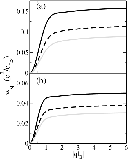
Figure 3: Dispersion relations of the bosons as a function of the momentum ${\bf q}$ with $\gamma=0$, in units of $e^{2}/\epsilon l_{B}$, when (a) $\nu=1/3$ and (b) $\nu=1/5$. The solid line corresponds to Eq. (45), whereas the dashed and solid gray lines represent the results for the width parameters $\lambda=0.5$ and $1.0$, respectively.

In order to include finite-width effects, we replace the bare Coulomb potential (14) by

$$v_{0}^{\lambda}(q)=\frac{2\pi e^{2}}{\epsilon q}e^{-|ql_{B}|^{2}/2}e^{|q\lambda|^{2}}\left[1-{\rm Erf}(\lambda q)\right],$$

where ${\rm Erf}(x)$ is the error function.arfken This expression has been obtained under the assumption that the confining potential in the $z$-direction (with a characteristic width $\lambda$, in units of $l_{B}$) is quadratic. MS ; shankar ; morf After replacing $v_{0}(q)\rightarrow v_{0}^{\lambda}(q)$, the momentum integral in Eq. (44) is evaluated numerically. For $\nu=1/3$ and $1/5$, the results for two different values of the width parameter ($\lambda=0.5$ and $1.0$, dashed and gray lines, respectively) are shown in Figs. 3 (a) and (b).

Notice that, in agreement with results by Murthy, the energy of the bosons decreases as $\lambda$ increases.murthy In fact, the finite-width results are likely to be more reliable than the ones at $\lambda=0$ as the preferred combination for the charge density [Eq. (II.2)] is derived in the long-wavelength limit, and the inclusion of finite-width effects cuts off the short-range contributions of the Coulomb potential.

From the experimental point of view, spin reversal excitations of the FQHE system have been studied with the help of inelastic light scattering.kang ; dujvone1 ; dujvone2 In this case, it is possible to probe some critical points of the dispersion relation of the neutral excitation, namely the ones at $q\rightarrow 0$ and $q\rightarrow\infty$. In particular, the latter can be probed because the wavevector is no longer conserved in the presence of residual disorder. The experimental spectrum at $\nu=1/3$ consists of five different peaks.dujvone1 ; dujvone2 Three of them have been associated to the charge modes at $q\rightarrow 0$ ($\Delta_{0}$), $q\rightarrow\infty$ ($\Delta_{\infty}$), and to the magnetoroton minimum. The one at the Zeeman energy has been associated to the long-wavelength limit of the spin-wave excitations, while the one between $\Delta_{0}$ and $\Delta_{\infty}$ was related to $E_{ph}$. In this case, it was estimated that $E_{ph}^{C}=0.054\;e^{2}/\epsilon l_{B}$. We obtain precisely this value for a width parameter $\lambda=3.0$, which corresponds to $290\,$Å at $B=7\,$T ($l_{B}=97\,$Å). In view of the approximations made (no Zeeman splitting, restriction to a single CF-LL level, and neglecting impurity effects), this is surprisingly close to the experimental situation, where a quantum well of width $330\,$Å was investigated at $7\,$T.dujvone1 ; dujvone2

III.2 Bound States of Two Bosons

Apart from the fact that our bosonization scheme reproduces the time-dependent Hartree-Fock (or RPA) results, it goes beyond as it yields an interacting bosonic model (41). Such kind of result was first derived for the 2DEG at $\nu=1$ in Ref. doretto, . In this section, we follow the lines of this work and study two-boson states in the interacting bosonic model in order to find out a relation between the two-boson bound states and the quasiparticle-quasihole (small skyrmion-antiskyrmion) pair excitations.

Finite-width effects are not considered here, and we therefore study the bosonic model (41) with the dispersion relation of the bosons given by Eq. (45). In order to study two-boson states, one needs to solve the Schrödinger equation

$$\mathcal{H}|\Phi_{\mathbf{P}}\rangle=E_{\mathbf{P}}|\Phi_{\mathbf{P}}\rangle,$$ (48)

where $|\Phi_{\mathbf{P}}\rangle$ is the more general representation of a two-boson state with total momentum ${\bf P}$, namely

$$|\Phi_{\mathbf{P}}\rangle=\sum_{\mathbf{q}}\Phi_{\mathbf{P}}(\mathbf{q})b^{\dagger}_{\mathbf{\frac{P}{2}-q}}b^{\dagger}_{\mathbf{\frac{P}{2}+q}}|FM\rangle.$$ (49)

Here, ${\bf P}$ is a good quantum number because the total momentum of a 2D system of charged particles in an external magnetic field is conserved when the total charge of the two-particle state is zero.osborne

Substituting Eq. (49) into (48) we obtain the following eigenvalue equation

$$[\varepsilon-E_{\mathbf{P}}(\mathbf{q})]\Phi_{\mathbf{P}}(\mathbf{q})=\int d^{2}k\,K_{\mathbf{P}}(\mathbf{k-q,q})\Phi_{\mathbf{P}}(\mathbf{k}),$$ (50)

where $E_{\bf P}({\bf q})=w_{{\bf P}/2-{\bf q}}+w_{{\bf P}/2+{\bf q}}$ is the energy of two free bosons, $\varepsilon=E_{\mathbf{P}}-E_{FM}$, and the kernel of the integral equation reads

$$K_{\mathbf{P}}(\mathbf{k-q,q}) = \frac{2}{\pi}\frac{e^{2}}{\epsilon l_{B}}\frac{e^{-|\mathbf{k-q}|^{2}/2(1-c^{2})}}{|\mathbf{k-q}|}\left[F^{CF}_{0}(|{\bf k}-{\bf q}|)\right]^{2}$$ (51)

$$\times\sin\left(\frac{(\mathbf{k-q})\wedge(\mathbf{P}/2+\mathbf{q})}{2(1-c^{2})}\right)$$

$$\times\sin\left(\frac{(\mathbf{k-q})\wedge(\mathbf{P}/2-\mathbf{q})}{2(1-c^{2})}\right).\;\;\;\;\;$$

In the above expressions, all momenta are measured in units of the inverse of the magnetic length $l_{B}^{-1}$.

The eigenvalues of (50) are evaluated numerically, using the quadrature technique.arfken In this case, the integral over momenta in (50) is replaced by a set of algebraic equations,

$$[\varepsilon-E_{\mathbf{P}}(\mathbf{q_{i}})]\Phi_{\mathbf{P}}(\mathbf{q_{i}})\approx\sum_{j\not=i}C_{j}K_{\mathbf{P}}(\mathbf{q_{j}-q_{i},q_{i}})\Phi_{\mathbf{P}}(\mathbf{q_{j}}),$$ (52)

and the eigenvalues for a fixed momentum ${\bf P}$ may be calculated by means of usual matrix techniques. The coefficients of the quadrature $C_{j}$ and the points ${\bf q}_{j}$ depend on the parametrization. We chose the one with $61$ points, which is used to calculate two-dimensional integrals over a circular region.stroud A cut-off for large momenta has to be introduced in order to define the region of integration. Therefore, only bosons with $|ql_{B}|<1$ are included in our calculations, and we concentrate on the analysis of the lowest-energy two-boson state. Both restrictions are related to the limitations of the numerical method.

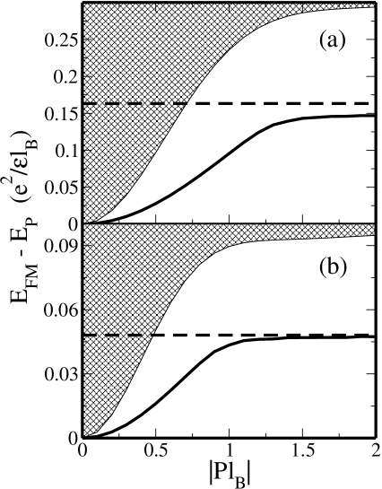
Figure 4: Dispersion relations of the two-boson state as a function of the total momentum ${\bf P}$, with $\gamma=0$, in units of $e^{2}/\epsilon l_{B}$, when (a) $\nu=1/3$ and (b) $1/5$. The solid line corresponds to the lowest-energy state of two bosons, the dashed line is the energy of a well-separated CF quasiparticle-quasihole [Eq. (46)], and the shaded area represents the continuum of scattering states.

In Figs. 4 (a) and (b), we show the lowest-energy state of two bosons (solid line) as a function of the total momentum ${\bf P}$ for $\nu=1/3$ and $1/5$, respectively, in units of $e^{2}/\epsilon l_{B}$, in the limit of $\gamma=0$. The shaded area corresponds to the continuum of scattering states. Because the solid line is below the band of scattering states, we may interpret the lowest energy eigenvalue ($E_{\bf P}$) as a bound state of two bosons. We have also included (dashed line) the value of the energy $E^{C}_{ph}$ of a CF-quasiparticle-quasihole pair [Eq. (46)], with the particle and the hole far apart from each other. Notice that in both cases, the asymptotic limit ($|{\bf P}|\rightarrow\infty$) of $E_{\bf P}$ is close to $E^{C}_{ph}$. In analogy with the 2DEG at $\nu=1$,doretto the bound state of two bosons with large ${\bf P}$ may be understood, for instance, as a CF quasiparticle bound to one spin wave plus a distant CF quasihole.doretto In this scenario, our results indicate that the creation of a CF quasiparticle dressed by a spin wave (or alternatively, a small skyrmion of CFs) is more favorable for the FQHE system at $\nu=1/3$ than for the one at $\nu=1/5$ as $|E^{C}_{ph}-E_{P\rightarrow\infty}|$ is smaller in the latter case. At present, no Knight-shift data are available for FQHE systems at $\nu=1/5$ to check our theoretical results.

The energy of small CF skyrmions for FQHE systems at $\nu=1/3$ and $1/5$ has been calculated numerically by Kamilla et al.,kamilla using a hard-core wavefunction.macdonald However, it is not possible to compare our results, namely, the asymptotic limit of $E_{\bf P}$, to the ones obtained by Kamilla and co-workers as they have evaluated the energy only of the positively charged excitation. In contrast to the 2DEG at $\nu=1$, the particle-hole symmetry is broken at $\nu=1/3$ and $1/5$. Therefore, the energy of the positive excitation cannot be used to estimate the energy of the negative one, and consequently the energy of a well-separated skyrmion-antiskyrmion pair cannot be determined. The breaking of the particle-hole symmetry at $\nu=1/3$ may be observed in the Knight-shift data, which are asymmetric around this filling factor.khandelwal2

IV Skyrmions of CFs

It has been shown in Ref. doretto, that the semi-classical limit of the interacting bosonic model provides a microscopic basis for a phenomenological model used by Sondhi et al.sondhi for the description of quantum Hall skyrmions. Sondhi’s model is given by the Lagrangian density

$$\mathcal{L}_{eff} = \frac{1}{2}\rho_{0}\mathcal{A}(\mathbf{n})\cdot\partial_{t}\mathbf{n}-\frac{1}{2}\rho_{S}(\mbox{\boldmath$\nabla$}\mathbf{n})^{2}+\frac{1}{2}\gamma\rho_{0}\mu_{B}\mathbf{n}\cdot\mathbf{B}$$ (53)

$$-\frac{e^{2}}{2\epsilon}\int d^{2}r^{\prime}\frac{q(\mathbf{r})q(\mathbf{r}^{\prime})}{|\mathbf{r}-\mathbf{r}^{\prime}|},$$

where $\rho_{S}$ is the spin stiffness,comment1 $\mathcal{A}(\mathbf{n})$ is the vector potential of a unit monopole ($\epsilon^{abc}\partial_{a}\mathcal{A}_{b}=n^{c}$) and $\rho_{0}=\nu/(2\pi l_{B}^{2})$ is the average electronic density. The topological charge or skyrmion density is given by

$$q(\mathbf{r})=\frac{1}{8\pi}\epsilon^{\alpha\beta}\mathbf{n}\cdot(\partial_{\alpha}\mathbf{n}\times\partial_{\beta}\mathbf{n}),$$ (54)

with $a,b,c=x,y,z$ and $\alpha,\beta=x,y$. Within the bosonization approach, the gradient, Zeeman and interaction terms of the above Lagrangian density have been derived, and one obtains, from a microscopic description, exactly the same coefficients. This result corroborates the relation between the bound state of two bosons and the small skyrmion-antiskyrmion pair excitation discussed in Ref. doretto, . In other words, the interacting bosonic model may be used to describe the quantum Hall skyrmion at $\nu=1$.

Here, we proceed in the same manner in order to derive the analogue of Sondhi’s model for the CF skyrmion at $\nu=1/(2s+1)$. We analyze the bosonic model (41), with the dispersion relation of the bosons given by Eq. (45).

Following the lines of Ref. moon, , we describe the CF skyrmion by the coherent state

$$|sk^{CF}(\mathbf{n})\rangle=\exp(-i\hat{O})|FM\rangle,$$ (55)

where the operator $\hat{O}$ is a non-uniform spin rotation which reorients the local spin from the direction $\mathbf{e}_{z}$ to $\mathbf{n}(\mathbf{r})$,

$$\hat{O} = \int d^{2}r\;\mathbf{\Omega}(\mathbf{r})\cdot\mathbf{S}(\mathbf{r})$$ (56)

$$= \int d^{2}q\;\left[\Omega^{+}(\mathbf{q})S^{-}_{-\mathbf{q}}+\Omega^{-}(\mathbf{q})S^{+}_{-\mathbf{q}}\right].$$

Here, $\mathbf{S}(\mathbf{r})$ is the spin operator, $\mathbf{n}(\mathbf{r})$ is a unit vector, and $\mathbf{\Omega}(\mathbf{r})=\mathbf{e}_{z}\times\mathbf{n}(\mathbf{r})$ defines the rotation angle. We assume that $\mathbf{\Omega(\mathbf{r})}$ describes small tilts away from the $\mathbf{e}_{z}$ direction, i.e. $\Omega^{\pm}(\mathbf{q})$ vanishes when $|ql_{B}|\gg 1$.

Using the expression for the spin density operator in terms of the boson operator $b$,comment2 the operator $\hat{O}$ becomes

$$\hat{O}\equiv\beta\sum_{{\bf q}}\left[\Omega^{+}_{\mathbf{q}}b^{\dagger}_{-\mathbf{q}}+\Omega^{-}_{{\bf q}}b_{\bf q}\right],$$ (57)

and the constant $\beta$ will be defined later.

We start with the analysis of the CF density operator (III). The average value of this operator in the state (55) is

$$\langle\bar{\bar{\rho}}({\bf k})\rangle = 2i\beta F^{0}_{CF}(k)$$ (58)

$$\times\sum_{\bf q}\sin\left(\mathbf{k}\wedge\mathbf{q}l^{*2}/2\right)\Omega^{-}_{{\bf k}+{\bf q}}\Omega^{+}_{-{\bf q}}.$$

Because only the long-wavelength limit of the theory is considered, one may approximate

$$\sin\left(\mathbf{k}\wedge\mathbf{q}l^{*2}/2\right)\approx\mathbf{k}\wedge\mathbf{q}l^{*2}/2=(\mathbf{k}\times\mathbf{q})_{z}l^{*2}/2,$$

and the CF form factor $F^{0}_{CF}(k)\approx 1-c^{2}$.

This implies that we only retain terms $\mathcal{O}(k^{2})$ in Eq. (58). Replacing the sum over momenta by an integral, and using the relation between the vector $\mathbf{\Omega}({\bf r})$ and the unit vector field $\mathbf{n}({\bf r})$, the average value of the CF density may be written as

$$\langle\bar{\bar{\rho}}({\bf k})\rangle = (1-c^{2})\frac{iN^{*}_{\phi}\beta^{2}(l^{*})^{4}}{2\pi}\int d^{2}q\;\mathbf{e}_{z}\cdot\left[(\mathbf{k}+\mathbf{q})\Omega^{-}_{\mathbf{k}+\mathbf{q}}\times\mathbf{q}\Omega^{+}_{\mathbf{q}}\right]$$ (59)

$$= -(1-c^{2})2\pi N^{*}_{\phi}\beta^{2}(l^{*})^{4}\int d^{2}r\;e^{-i\mathbf{k}\cdot\mathbf{r}}\mathbf{e}_{z}\cdot\left(\mbox{\boldmath$\nabla$}n^{x}\times\mbox{\boldmath$\nabla$}n^{y}-\mbox{\boldmath$\nabla$}n^{y}\times\mbox{\boldmath$\nabla$}n^{x}\right),$$

and therefore, its Fourier transform becomes

$$\langle\bar{\bar{\rho}}({\bf r})\rangle=-(1-c^{2})2\pi N^{*}_{\phi}\beta^{2}(l^{*})^{4}\mathbf{e}_{z}\cdot\left(\mbox{\boldmath$\nabla$}n^{x}\times\mbox{\boldmath$\nabla$}n^{y}-\mbox{\boldmath$\nabla$}n^{y}\times\mbox{\boldmath$\nabla$}n^{x}\right).$$ (60)

Notice that, if we choose the constant $\beta=1/\left(4\pi\sqrt{N^{*}_{\phi}}(l^{*})^{2}\right)$ the average value of the CF density is equal to the topological charge times the filling factor $\nu=(1-c^{2})=1/(2s+1)$, as suggested by Sondhi et al. in Ref. sondhi, . With this choice, we may calculate the average value of the energy in the state (55), considering the interacting bosonic model (41), with $w_{\bf q}$ as in Eq. (45).

The average value of the quadratic term of the Hamiltonian (41) is given by

$$\langle sk^{CF}|\hat{H}_{0}^{B}|sk^{CF}\rangle = \frac{1}{16\pi^{2}N^{*}_{\phi}(l^{*})^{4}}\sum_{\bf q}w_{\mathbf{q}}\Omega^{+}_{-\mathbf{q}}\Omega^{-}_{\mathbf{q}}.$$

Because the long-wavelength limit of the dispersion relation of the bosons [Eq. (45)] is

$$w_{\bf q}\approx\gamma+\frac{e^{2}}{l_{B}\epsilon}\sqrt{1-c^{2}}\sqrt{\frac{\pi}{2}}\frac{1}{4}\tilde{\alpha}(c)|ql^{*}|^{2},$$ (61)

with the constant

$$\tilde{\alpha}(c)=1-2c^{5}+\frac{c^{7}}{(2-c^{2})^{3/2}},$$ (62)

the average value of $\hat{H}_{0}^{B}$ is

$$\langle\mathcal{H}_{0}\rangle \approx \frac{1}{2}\rho_{S}\int d^{2}r\;\left[\mbox{\boldmath$\nabla$}\mathbf{n}(\mathbf{r})\right]^{2}$$ (63)

$$-\frac{1}{2}g^{*}\mu_{B}\frac{1}{2\pi(l^{*})^{2}}\int d^{2}r\;\mathbf{n}\cdot\mathbf{B}$$

$$+\frac{1}{2}g^{*}\mu_{B}B\frac{1}{2\pi}N^{*}_{\phi}.$$

Here, the spin stiffness is defined as

$$\rho_{S}=\frac{1}{16\pi}\frac{e^{2}}{\epsilon l^{*}}\sqrt{\frac{\pi}{2}}\tilde{\alpha}(c)=\rho_{S}^{*}\mu(c),$$ (64)

with

$$\rho_{S}^{*}\equiv\frac{1}{16\pi}\frac{e^{*2}}{\epsilon l^{*}}\sqrt{\frac{\pi}{2}}$$ (65)

and $\mu(c)=\tilde{\alpha}(c)/(1-c^{2})^{2}$. Notice that one would have obtained the value $\rho_{S}^{*}$ for the CF spin stiffness simply by replacing $e\rightarrow e^{*}$ and $l_{B}\rightarrow l^{*}$ in the expression for the electronic spin stiffness at $\nu=1$.sondhi This corresponds to a CF mean-field approach,nakajima and $\mu(c)$ may thus be interpreted as a mismatch factor with respect to the mean-field result.

Performing an analogous calculation for the quartic term of the Hamiltonian (41), one finds

$$\langle\hat{H}_{I}\rangle = {\cal N}\sum_{\mathbf{k,p,q}}v_{0}(k)\left[F_{0}^{CF}(k)\right]^{2}\sin(\mathbf{k}\wedge\mathbf{p}l^{*2}/2)$$

$$\times\sin(\mathbf{k}\wedge\mathbf{q}l^{*2}/2)\Omega^{-}_{\mathbf{k}+\mathbf{q}}\Omega^{-}_{\mathbf{p}-\mathbf{k}}\Omega^{+}_{-\mathbf{p}}\Omega^{+}_{-\mathbf{q}}$$

$$\approx \frac{(1-c^{2})^{2}}{2}\int d^{2}r\,d^{2}r^{\prime}\;V(\mathbf{r}-\mathbf{r^{\prime}})q(\mathbf{r})q(\mathbf{r^{\prime}}),$$

where ${\cal N}=2/\left(\mathcal{A}(4\pi)^{4}N^{*2}_{\phi}(l^{*})^{8}\right)$. Therefore, using equations (63) and (LABEL:energyskyrmion2), one obtains the average value of the total Hamiltonian with respect to the state $|sk^{CF}\rangle$

$$\langle\hat{H}\rangle = \frac{1}{2}\rho^{0}_{S}\int d^{2}r\;\left[\mbox{\boldmath$\nabla$}\mathbf{n}(\mathbf{r})\right]^{2}+\frac{1}{2}g^{*}\mu_{B}B\frac{1}{2\pi}N^{*}_{\phi}$$ (67)

$$-\frac{1}{2}g^{*}\mu_{B}\frac{1}{2\pi l^{*2}}\int d^{2}r\;\mathbf{n}\cdot\mathbf{B}$$

$$+\frac{e^{2}(1-c^{2})^{2}}{2}\int d^{2}r\,d^{2}r^{\prime}\;\frac{q(\mathbf{r})q(\mathbf{r^{\prime}})}{|\mathbf{r}-\mathbf{r^{\prime}}|}\;\;\;\;$$

Eq. (67) corresponds to an energy functional of a static configuration of the vector field $\mathbf{n}({\bf r})$, derived from a Lagrangian density similar to (53). Notice that the coefficient of the Zeeman term,

$$\frac{g^{*}\mu_{B}}{2}\frac{\nu^{*}}{2\pi l^{*2}}=\frac{g^{*}\mu_{B}}{2}\frac{\nu}{2\pi l_{B}^{2}},$$

is identical to that of Sondhi et al.,sondhi with the difference that here, this term is derived from first principles and not assumed phenomenologically. Furthermore, the last term in Eq. (67) accounts for the Coulomb interaction between CF-quasiparticles with effective charge $e^{*}=e(1-c^{2})$.

The analysis of the semi-classical limit of the interacting bosonic model (41) allows us to calculate analytically the spin stiffness. From Eq. (64), one obtains

$$\rho_{S}=\left\{\begin{array}[]{r@{\quad}l}6.207\times 10^{-3}&\nu=1/3,\\ 2.269\times 10^{-3}&\nu=1/5,\end{array}\right.$$ (68)

in units of $e^{2}/\epsilon l_{B}$.

There is a set of different values for the spin stiffness at $\nu=1/3$ and $1/5$ available in the literature. Based on Ref. mandal, , Mandal and Ravishankarmandal2 estimated that the spin stiffnesses at $\nu=1/3$ and $1/5$ are equal to $1.591\times 10^{-3}$ and $4.774\times 10^{-4}\;e^{2}/\epsilon l_{B}$, respectively. These values are derived from the spin stiffness at $\nu=1$ with the replacements $e\rightarrow e^{*}$ and $l_{B}\rightarrow l^{*}$, and may be interpreted as the mean-field values of the CF spin stiffness, as indicated above. In fact, these results are in agreement with estimates by Sondhi et al.sondhi The spin stiffness has also been calculated numerically by Moon et al.,moon using the hypernetted-chain-approximation.macdonald2 In this case, it was found that $\rho_{S}=9.23\times 10^{-4}\;\;[\nu=1/3]$ and $2.34\times 10^{-4}\;e^{2}/(\epsilon l_{B})\;\;[\nu=1/5]$. Those values are also considered by Lejnell et al.lejnell in the study of the quantum Hall skyrmion. Furthermore, the spin stiffness at $\nu=1/3$ as a function of temperature and finite width has been estimated by Murthymurthy2 in the Hartree-Fock approximation of the Hamiltonian theory. At low temperatures ($0<T<2\;K$), one finds $\rho_{S}(T)\approx 2.125\times 10^{-3}$.

The values we obtain with the help of the bosonization approach in the Hamiltonian theory are larger than the theoretical estimates found in the literature. In the case of the mean-field values obtained by Sondhi et al.sondhi and Mandal and Ravishankar,mandal2 the mismatch is given by the factor $\mu(c)$, which is $3.9$ at $\nu=1/3$ and $5.1$ at $\nu=1/5$. The origin of this mismatch is the Gaussian $\exp(-|ql_{B}|^{2}/2c^{2})$ in the CF form factor (25), which takes into account the difference between the magnetic length of the electron and that of the pseudo-vortex, which constitute the CF.MS The mismatch is thus due to the internal structure of the CF, which is not taken into account in a mean-field approximation, where the CF is considered as a pointlike particle with charge $e^{*}$.

A comparison with experimental data has only been done in Ref. murthy2, , where the temperature dependence of the spin polarization at $\nu=1/3$ has been evaluated, using the continuum quantum ferromagnet model in the large-$N$ approach. In this work, the two free parameters of the model (spin stiffness and magnetization density) have been taken temperature-dependent. This formalism had previously been used to describe the spin polarization of the 2DEG at $\nu=1$,read but with constant parameters. The agreement between the theoretical result and the experimental data,khandelwal2 even when only the zero-temperature values of two free parameters were taken into account, indicated that, within this formalism, the estimated value of the spin stiffness is quite reasonable. Although we find a larger value for the spin stiffness than Murthy’s, it can be reduced if finite-width effects are included in the model. Remember that the preferred combination of the CF density is less accurate at larger momenta and the inclusion of finite-width effects softens the short-range terms of the interaction potential.

Finally, the energy of the CF skyrmion ($E_{sk}$) may also be estimated in the long-wavelength limit. The leading term of the skyrmion energy is $4\pi\rho_{S}$,sondhi which is basically the energy of the skyrmion in the limit of zero Zeeman energy. One obtains from the values (68)

$$E_{sk}=\left\{\begin{array}[]{r@{\quad}l}0.078&\nu=1/3,\\ 0.028&\nu=1/5,\end{array}\right.$$ (69)

in units of $e^{2}/\epsilon l_{B}$. These results are in agreement with the energy of a large (number of spin reversals) skyrmion calculated by Kamilla et al.kamilla This indicates that the hard-core wavefunction description for the CF skyrmion and the Hamiltonian theory in the bosonization approach converge in the long-wavelength limit.

V Summary

In conclusion, we have calculated neutral spin excitations of FQHE systems at $\nu=1/(2s+1)$, using a bosonization approach for the Hamiltonian theory of the FQHE proposed by Murthy and Shankar.MS The generalization of this formalism with the inclusion of a discrete degree of freedom has been presented, under the assumption that one may neglect higher CF levels, which are separated from the ground state by a larger gap than the spin-level splitting ($\gamma\rightarrow 0$ limit).

Because in the CF picture the electronic system at $\nu=1/(2s+1)$ is described by a CF model with effective filling factor $\nu^{*}=1$, we can apply the bosonization method for the 2DEG at $\nu=1$, recently developed by two of us.doretto In this case, the neutral spin excitations of the system are treated as bosons, and the original interacting CF model is mapped onto an interacting bosonic one.

The dispersion relation of the bosons (neutral spin reversal excitations) has been evaluated analytically for an ideal system, neglecting finite-width, Landau-level-mixing and disorder effects. We have illustrated the results for FQHE systems at $\nu=1/3$ and $\nu=1/5$. The bosonization approach allows us to calculate analytically the energy of the spin excitations over the whole momentum range.

Our results agree with numerical investigations in the time-dependent Hartree-Fock approximation.murthy We have shown that the long-wavelength limit of the bosonic dispersion relation corresponds to spin-wave excitations of the quantum Hall ferromagnet of CFs, which is the ground state of the system. The energies of the spin waves are larger than those obtained in previous theoretical studies by Nakajima and Aoki.nakajima The large-wavevector limit of the dispersion relation is related to the energy to create a CF-quasiparticle-quasihole pair ($E_{ph}$), the constituents of which are far apart from each other. Our results are also larger than numerical ones obtained with the help of trial wavefunctions for the excited state in the CF picture mandal-jain and exact-diagonalization studies on systems with a few number of particles.rezayi2 Even if these values occur to be closer than ours to experimental estimatesdujvone1 ; dujvone2 of the $E_{ph}$, an excellent agreement is obtained when finite-width effects are taken into account. Indeed, the width of the quantum well used in the experiments corresponds to a width parameter $\lambda\sim 3l_{B}$ ($\sim 300\,$Å at $7\,$T), for which we obtain a reduction of $E_{ph}$ roughly by a factor of three. Note that finite-width results are more reliable in the Hamiltonian theory, which was originally derived in the long-wavelength limit, than that for the ideal 2D case because, in this case, short-range contributions of the interaction potential are suppressed.murthy This cuts off short-wavelength fluctuations and thus brings the model back to its regime of validity.

In the framework of the interacting bosonic model, we have shown that the interaction potential between the bosons accounts for the formation of two-boson bound states. As in the case of the 2DEG at $\nu=1$, the two-boson bound state is interpreted in terms of a small CF-skyrmion-antiskyrmion pair excitation. FQHE systems at $\nu=1/3$ and $1/5$ have been investigated. Based on the relation between the asymptotic limit of the energy of the lowest two-boson bound state and $E_{ph}$, we conclude that a CF quasiparticle dressed by spin waves is more stable than a bare CF quasiparticle only at $\nu=1/3$. Experimental results at $\nu=1/5$, such as Knight shift data, are lacking at the moment and may give further insight into the spin-excitation spectrum of this state.

Finally, we have shown that the semi-classical limit of the interacting bosonic model yields an energy functional derived from a Langrangian density, similar to the phenomenological one considered by Sondhi et al.sondhi for the study of the quantum Hall skyrmion. We thus corroborate the relation between the two-boson bound state and small skyrmion-antiskyrmion pair excitations.

- (1) S. Das Sarma and A. Pinczuk, eds., Perspectives in Quantum Hall Effects, Wiley, New York (1997).
- (2) J. K. Jain, Phys. Rev. Lett. 63, 199 (1989); Phys. Rev. B 41, 7653 (1990).
- (3) O. Heinonen, ed., Composite Fermions, World Scientific, Singapore (1998).
- (4) R. B. Laughlin, Phys. Rev. Lett. 50, 1395 (1983).
- (5) A. Lopez and E. Fradkin, Phys. Rev. B 44, 5246 (1991).
- (6) B. I. Halperin, P. A. Lee, and N. Read, Phys. Rev. B 47, 7312 (1993).
- (7) R. Shankar and G. Murthy, Phys. Rev. Lett. 79, 4437 (1997); G. Murthy and R. Shankar, in Ref. heinonen, ; G. Murthy and R. Shankar, Rev. Mod. Phys. 75, 1101 (2003).
- (8) T. H. R. Skyrme, Proc. R. Soc. London Ser. A 247, 260 (1958).
- (9) D. H. Lee and C. L. Kane, Phys. Rev. Lett. 64, 1313 (1990).
- (10) S. L. Sondhi, A. Karlhede, S. A. Kivelson, and E. H. Rezayi, Phys. Rev. B 47, 16419 (1993).
- (11) K. Moon, H. Mori, Kun Yang, S. M. Girvin, A. H. MacDonald, L. Zheng, D. Yoshioka, and Shou-Cheng Zhang, Phys. Rev. B 51, 5138 (1995).
- (12) S. E. Barrett, G. Dabbagh, L. N. Pfeiffer, K. W. West, and R. Tycko, Phys. Rev. Lett. 74, 5112 (1995).
- (13) R. L. Doretto, A. O. Caldeira, and S. M. Girvin, Phys. Rev. B 71, 045339 (2005).
- (14) J. von Delf and H. Schoeller, Ann. Phys. (Leipzig) 7, 225 (1998).
- (15) J. Voit, Rep. Prog. Phys. 58, 977 (1995).
- (16) A. H. Castro Neto and E. Fradkin, Phys. Rev. B 49, 10877 (1994).
- (17) A. Houghton and J. B. Marston, Phys. Rev. B 48, 7790 (1993).
- (18) H. Westfahl Jr., A. H. Castro Neto, and A. O. Caldeira, Phys. Rev. B 55, R7347 (1997).
- (19) P. Khandelwal, N. N. Kuzma, S. E. Barrett, L. N. Pfeiffer, and K. W. West, Phys. Rev. Lett. 81, 673 (1998).
- (20) I. Stanić and M. V. Milovanović, Phys. Rev. B 71, 035329 (2005).
- (21) D. Bohm and D. Pines, Phys. Rev. 92, 609 (1953).
- (22) C. L. Kane, S. Kivelson, D.-H. Lee, and S.-C. Zhang, Phys. Rev. B 43, 3255 (1991).
- (23) B. L. Halperin, Helv. Phys. Acta 56, 75 (1983).
- (24) S. M. Girvin and T. Jach, Phys. Rev. B 29, 5617 (1984).
- (25) R. Shankar, Phys. Rev. B 63, 085322 (2001).
- (26) S. M. Girvin, A. H. MacDonald, and P. M. Platzman, Phys. Rev. B 33, 2481 (1986).
- (27) V. Pasquier and F. D. M. Haldane, Nucl. Phys. B 516, 719 (1998).
- (28) B. I. Halperin and A. Stern, Phys. Rev. Lett. 80, 5457 (1998); G. Murthy and R. Shankar, ibid. 80, 5458 (1998); ibid. 79, 4437 (1997).
- (29) M. O. Goerbig, P. Lederer, and C. Morais Smith, Phys. Rev. B 69, 155324 (2004); Europhys. Lett. 68, 72 (2004).
- (30) S. Tomonaga, Prog. Theor. Phys. 5, 544 (1950).
- (31) G. Arfken and H. J. Weber, Mathematical methods for physicists, Academic Press (1995).
- (32) G. Murthy, Phys. Rev. B 60, 13702 (1999).
- (33) P. Nozières and D. Pines, The theory of quantum liquids, (Perseus books, 1999).
- (34) T. Nakajima and H. Aoki, Phys. Rev. Lett. 73, 3568 (1994).
- (35) C. Kallin and B. I. Halperin, Phys. Rev. B 30, 5655 (1984).
- (36) S. S. Mandal, Phys. Rev. B 56, 7525 (1997).
- (37) S. S. Mandal and J. K. Jain, Phys. Rev. B 64, 125310 (2001).
- (38) E. H. Rezayi, Phys. Rev. B 36, 5454 (1987).
- (39) R. Morf and N. d’Ambrumenil, Phys. Rev. B 68, 113309 (2003).
- (40) M. Kang, A. Pinczuk, B. S. Dennis, M. A. Eriksson, L. N. Pfeiffer, and K. W. West, Phys. Rev. Lett. 84, 546 (2000).
- (41) I. Dujovne, A. Pinczuk, M. Kang, B. S. Dennis, L. N. Pfeiffer, and K. W. West, Phys. Rev. Lett. 90, 036803 (2003).
- (42) I. Dujovne, C. F. Hirjibehedin, A. Pinczuk, M. Kang, B. S. Dennis, L. N. Pfeiffer, and K. W. West, Solid State Commun. 127, 109 (2003).
- (43) J. L. Osborne, A. J. Shields, M. Y. Simmons, N. R. Cooper, D. A. Ritchie, and M. Pepper, Phys. Rev. B 58, R4227 (1998).
- (44) A. H. Stroud, Approximate calculation of multiple integrals, Prentice-Hall series in automatic computation (1971).
- (45) R. K. Kamilla, X. G. Wu, and J. K. Jain, Solid State Commun. 99, 289 (1996).
- (46) A. H. MacDonald, H. A. Fertig, and L. Brey, Phys. Rev. Lett. 76, 2153 (1996).
- (47) At , , in units of .
- (48) Although the bosonic representation of the CF spin density operators are not derived here, they are similiar to the ones derived in Ref. doretto, for the 2DEG at , without the Gaussian factors .
- (49) S. S. Mandal and V. Ravishankar, Phys. Rev. B 57, 12333 (1998).
- (50) A. H. MacDonald, G. C. Aers, and M. W. C. Dharma-wardana, Phys. Rev. B 31, 5529 (1985).
- (51) K. Lejnell, A. Karlhede, and S. L. Sondhi, Phys. Rev. B 59, 10183 (1999).
- (52) G. Murthy, J. Phys.:Condens. Matter 12, 10543 (2000).
- (53) N. Read and S. Sachdev, Phys. Rev. Lett. 75, 3509 (1995).