The Kondo Effect in Non-Equilibrium Quantum Dots:
Perturbative Renormalization Group

Abstract

While the properties of the Kondo model in equilibrium are very well understood, much less is known for Kondo systems out of equilibrium. We study the properties of a quantum dot in the Kondo regime, when a large bias voltage $V$ and/or a large magnetic field $B$ is applied. Using the perturbative renormalization group generalized to stationary nonequilibrium situations, we calculate renormalized couplings, keeping their important energy dependence. We show that in a magnetic field the spin occupation of the quantum dot is non-thermal, being controlled by $V$ and $B$ in a complex way to be calculated by solving a quantum Boltzmann equation. We find that the well-known suppression of the Kondo effect at finite $V\gg T_{K}$ (Kondo temperature) is caused by inelastic dephasing processes induced by the current through the dot. We calculate the corresponding decoherence rate, which serves to cut off the RG flow usually well inside the perturbative regime (with possible exceptions). As a consequence, the differential conductance, the local magnetization, the spin relaxation rates and the local spectral function may be calculated for large $V,B\gg T_{K}$ in a controlled way.

1 Introduction

After 40 years of research, the single-impurity Kondo model[1] and its variants are certainly among the best understood strongly correlated systems. An amazingly broad spectrum of powerful theoretical methods[2] have been developed to describe the physics of a magnetic impurity in a metal, ranging from exact analytical solutions using the Bethe Ansatz, bosonization and conformal field theory, diagrammatic methods, flow equations, perturbative renormalization group to sophisticated numerical techniques like the numerical renormalization group. Using these tools an almost complete understanding of thermodynamic, transport and spectral properties of the single-impurity Kondo model has been achieved [2].

There is, however, one important field about which in comparison little is known: Kondo physics out of equilibrium, a question of both experimental and theoretical importance. Non-equilibrium can, for example, be reached when a finite current is driven through a Kondo system (see below).

The study of the Kondo effect out of equilibrium started both experimentally and theoretically in the late 1960’s when the tunneling between two metals through insulating barriers was investigated[6, 7, 3, 4, 5, 8] as a function of bias voltage. The observed logarithmic enhancement of the tunneling for low temperature and small voltages was attributed to exchange tunneling through magnetic impurities within the barriers by Appelbaum [9, 10] and Anderson[11]. The relevant impurities were argued[11] to reside close to one side of the junction, and the localized spin was therefore tacitly assumed to be in equilibrium with the metal closeby. The tunneling to the other metal is weak and the conductance in such a situation is determined by the equilibrium density of states on the impurity[12, 13]. Subsequent work by Ivezić[14] considered also impurities deep inside the junction, which were pointed out to require a full non-equilibrium treatment. A good review of these earlier works may be found in Ref. [15].

With the progress in nanotechnology, it became possible to realize Kondo physics in quantum dots[16, 17, 18, 19, 20, 21]. A dot in the Coulomb blockade regime which carries a net spin can be mapped to the Kondo model[22, 23]. The resonant tunneling through the dot leads to a removal of the Coulomb blockade, i.e. an increase of the conductance from small values up to the quantum limit, as the Kondo resonance develops. A finite bias voltage $V$ drives the system out of equilibrium. It has been observed that the Kondo effect is quenched by raising the transport bias voltage V well above the Kondo temperature $T_{K}$, i.e. $V\gg T_{K}$, and that the presence of a magnetic field splits the zero-bias conductance peak into two distinct peaks, located at bias voltages roughly equal to plus and minus the Zeeman splitting of the spin on the dot[16, 17, 18, 19, 20]. Similar experiments were also possible in metallic nanoconstrictions where it is possible to measure transport through a single magnetic impurity [24], however, in contrast to quantum dots it is not possible to control system parameters in such devices.

The most straightforward way to study quantum dots out of equilibrium is to apply a finite dc bias voltage and to measure the current-voltage characteristics. There have, however, been a few remarkable experiments which go further. For example, Franceschi et al. [25] managed to measure the splitting of the Kondo resonance by a dc bias voltage by using a three-lead configuration. Another set of questions can be addressed by studying the response to time-dependent external fields induced, for example, by external irradiation by a microwave field with frequency $\omega$ [26, 28, 29, 30, 31]. Kogan et al. [32] recently succeeded in observing satellites of the Kondo effect separated by $\omega$ in such an experiment.

Kondo impurities also have a pronounced effect on the distribution of electrons in mesoscopic wires, which are driven out of equilibrium by an applied bias voltage[33, 34, 35]. The inelastic scattering from the magnetic impurities at finite bias leads to a characteristic broadening[36, 37, 38] of the electronic distribution functions which can be measured in tunneling experiments[33, 34, 35].

Theoretically, the Kondo effect out of equilibrium has been studied by a number of methods ranging from perturbation theory [9, 10, 27, 12, 28, 46, 43, 44, 45, 39, 40, 41, 42], equations of motions and self-consistent diagrammatic methods [47, 48, 49, 30, 50, 51, 52, 53, 54, 55] (using the so-called non-crossing approximation), slave-boson mean-field theories [57, 58, 59], exact solutions for some variants of the Kondo model with appropriately chosen coupling constants [56], the construction of approximate scattering states starting from Bethe ansatz solutions[60], to perturbative renormalization group [28, 43, 61](reviewed below). It is, however, important to note, that many of the methods which have been so successful in equilibrium cannot or have not yet been generalized even to the simplest steady-state non-equilibrium situation. One of the reasons for this is that the current-carrying state at finite bias is a highly excited many-body state of the system. Therefore, all methods which by construction focus on ground state properties are not readily generalized to such a situation.

In the following sections, we will review our version [43] of perturbative renormalization group (RG) in the presence of a finite bias voltage – formulated in the spirit of Anderson’s poor man’s scaling [62]. We generalize the RG equations presented in Ref. [43] for a symmetric dot to an arbitrary exchange coupling of the spin to the conduction electrons of two attached leads with different electrochemical potential. The central goal is to perform a controlled calculation in the limit of either large bias voltage $V\gg T_{K}$ or large magnetic field $B\gg T_{K}$ or large probing frequency $\omega\gg T_{K}$. We suggest a method to calculate the behavior of the conductance and other physical quantities like magnetization or spectral function in leading order of the small parameter $1/\ln[\max(V,B,\omega)/T_{K}]$. We will argue that the perturbative renormalization group differs in three main aspects from its counterpart in equilibrium [62]: First, the magnetization of the Kondo impurity (or in general the occupation probabilities of the quantum states) has to be calculated self-consistently from appropriate quantum Boltzmann equations [46, 43, 44]. This leads to an unusual dependence e.g. of the spin susceptibility on $V$ and to a novel structure of the logarithmic corrections. Second, the perturbative renormalization group has to be formulated in terms of frequency-dependent coupling functions instead of coupling constants. The reason is that electrons in an energy window set approximately by the external bias voltage contribute to the low-energy properties (see Fig. 1) and their position within this window will affect their effective coupling to the spin. Therefore, the effective renormalized coupling of the conduction electrons to the local spin will depend explicitly on their energy. Third, decoherence effects are much more important out of equilibrium [63, 28, 55, 43, 45]. A finite current will induce noise and thereby induce dephasing of the coherent spin-flip processes responsible for the Kondo effect. We will show that it is precisely due to those dephasing effects that a controlled calculation at large voltages is possible.

2 Perturbation Theory

We consider the Kondo Hamiltonian

$$H=\sum_{\alpha=L,R,{\bf k},\sigma}(\varepsilon_{{\bf k}}-\mu_{\alpha})c^{\dagger}_{\alpha{\bf k}\sigma}c_{\alpha{\bf k}\sigma}-BS_{z}\\ +\frac{1}{2}\!\!\!\sum_{\alpha,\alpha^{\prime}=L,R,{\bf k},{\bf k}^{\prime},\sigma,\sigma^{\prime}}\!\!\!\!\!J_{\alpha^{\prime}\alpha}\,{\mathbf{S}}\cdot(c^{\dagger}_{\alpha^{\prime}{\bf k}^{\prime}\sigma^{\prime}}{\boldsymbol{\tau}}_{\sigma^{\prime}\sigma}c_{\alpha{\bf k}\sigma}),$$ (1)

where $\mu_{L,R}=\pm V/2$. ${\mathbf{S}}$ is the spin 1/2 on the dot and ${\boldsymbol{\tau}}$ are the Pauli matrices. This model describes a quantum dot coupled to two leads (the left and right electrons described by $c^{\dagger}_{L/R,{\bf k}\sigma}$) in which the number of electrons on the dot is fixed to an odd integer by an interplay of gate voltage and charging energy. In this Coulomb blockade regime, effectively a single spin is localized on the dot which interacts via an exchange coupling $J_{\alpha\alpha^{\prime}}$ arising from tunneling processes from and to the leads involving virtual excitation of the dot. In cases where the quantum dot can be described by a simple Anderson model, one obtains $J_{LR}=J_{RL}=\sqrt{J_{LL}J_{RR}}$. In more complex situations, $J_{\alpha\alpha^{\prime}}$ can be an arbitrary symmetric $2\times 2$ matrix. In general, a further cotunneling term $Vc^{\dagger}_{\alpha}c_{\alpha^{\prime}}$ exists. As such a term does not flow to strong coupling under renormalization group, it can be safely neglected (furthermore, such a term vanishes for an appropriate choice of a gate voltage in the middle of the Coulomb blockade valley). We shall use the dimensionless coupling constants $g_{\alpha\alpha^{\prime}}=N_{0}J_{\alpha\alpha^{\prime}}$, where $N_{0}$ is the local density of states in the leads. For simplicity, we have coupled in Eq. (1) the magnetic field (measured in units where $g\mu_{B}=1$) only to the local spin. An extra coupling to the electrons would effectively lead only to a small renormalization of the $g$ factor. We assume a constant density of states in the leads in a frequency range of order $B$ and $V$. In such a situation the density of states at the Fermi level remains unmodified in the presence of $B$.

In order to be able to use standard diagrammatic techniques, we represent the local spin ${\mathbf{S}}=\frac{1}{2}\sum_{\gamma\gamma^{\prime}}f^{\dagger}_{\gamma}{\boldsymbol{\tau}}_{\gamma\gamma^{\prime}}f_{\gamma^{\prime}}$ by pseudo-fermions in the sector of the Hilbert space with $\sum_{\gamma}f^{\dagger}_{\gamma}f_{\gamma}=1$. Details of the Keldysh diagrammatic method [64] used throughout this paper and how the exact projection to the physical Hilbert space of the pseudo Fermions is performed can be found in Ref. [44] where the perturbation theory for the Kondo model is derived in detail to leading logarithmic order.

Before setting up a renormalization group scheme, it is useful to investigate the results of perturbation theory, e.g. for the spin susceptibility. Out of equilibrium, the calculation of the susceptibility has to be done with some care, the bare perturbation theory diverges even at finite temperature $T$. Physicswise this arises because for $J=0$ the magnetization of the completely uncoupled dot is undetermined. While in equilibrium any infinitesimal coupling leads to the usual thermal occupation independent of all details of the coupling, this is not the case out of equilibrium, where the details of the coupling do matter. Practically this implies that one has to calculate the occupation function even in the limit of vanishing $J$ from some type of (quantum-) Boltzmann equation. In diagrammatics, this is given by one component of a (self-consistent) Dyson equation in Keldysh space (see Refs. [46, 44] for details). To lowest order this is just the well-known Boltzmann equation with golden-rule transition rates. To obtain the steady state, the spin-flip rate from $\uparrow$ to $\downarrow$ has to equal the rate in the opposite direction and therefore

$$n_{\uparrow}\sum_{\alpha,\alpha{{}^{\prime}}=L,R}g_{\alpha\alpha^{\prime}}^{2}\int d\omega\,f_{\omega-\mu_{\alpha}}\Big{(}1-f_{\omega-\mu_{\alpha{{}^{\prime}}}-B}\Big{)}=\\ =n_{\downarrow}\sum_{\alpha,\alpha{{}^{\prime}}=L,R}g_{\alpha\alpha^{\prime}}^{2}\int d\omega\,f_{\omega-\mu_{\alpha}}\Big{(}1-f_{\omega-\mu_{\alpha{{}^{\prime}}}+B}\Big{)}\ .$$ (2)

where $f_{\omega}$ is the Fermi function. Solving for $n_{\uparrow}-n_{\downarrow}$ in the limit $B\to 0$, one finds [46, 43, 44]

$$\chi = \frac{2g_{LR}^{2}+g_{LL}^{2}+g_{RR}^{2}}{2V\coth\left(\frac{V}{2T}\right)g_{LR}^{2}+2T(g_{LL}^{2}+g_{RR}^{2})}.$$ (3)

In equilibrium, $V=0$, all coupling constants cancel out and one obtains $\chi=1/(2T)$ to zeroth order in the coupling constants. For a finite voltage, however, the result depends on the ratio of the coupling constants even for infinitesimal $J_{\alpha\alpha^{\prime}}$. For large voltages one finds $\chi\sim 1/V$.

One order higher, the logarithmic correction characteristic for the Kondo effect[1] arises and one obtains [43, 44], with $g_{d}=(g_{LL}+g_{RR})/2$,

$$\hskip 42.67912pt\chi=\frac{2g_{LR}^{2}\left(1+2g_{d}\ln\frac{D}{T}+2g_{d}\ln\frac{D}{|V|}\right)+\sum_{\gamma}g_{\gamma\gamma}\left(g_{\gamma\gamma}+2g_{\gamma\gamma}^{2}\ln\frac{D}{T}+2g_{LR}^{2}\ln\frac{D}{|V|}\right)}{2V\coth\left(\frac{V}{2T}\right)g_{LR}^{2}\left(1+4g_{d}\ln\frac{D}{|V|}\right)+2T\sum_{\gamma}g_{\gamma\gamma}\left(g_{\gamma\gamma}+2g_{\gamma\gamma}^{2}\ln\frac{D}{T}+2g_{LR}^{2}\ln\frac{D}{|V|}\right)}\hskip 14.22636pt$$ (4)

where the bandwidth $D$ cuts off the logarithmic singularities at high energies. Note that logarithmic corrections arise already to linear order in $g$ with prefactors which again depend on the ratios of the coupling constants. In the limit of $T\gg V$, in contrast, the logarithms all take the form $\ln(D/T)$, the corrections in the numerator and in the denominator cancel, and we are left with the usual Curie law $\chi=1/2T$, as in equilibrium the first logarithmic correction arises only to order $g^{2}$, not included in Eq. (4). This shows again that in the presence of a finite bias voltage, the structure of perturbation theory is strongly modified.

3 Perturbative Renormalization Group

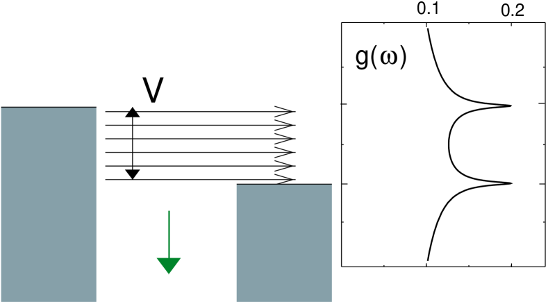
Figure 1: Due to the finite bias voltage, the electrochemical potential of the right and left lead differ by $V$. As all electrons in an energy window of width $V$ contribute to low energy properties, it is necessary to take into account that the effective exchange coupling of the electrons depends on their energy. Right panel: frequency dependent effective coupling $g(\omega)$ calculated from Eq. (28) for $V/T_{K}=100$.

Even for small coupling constants $g$ and for sufficiently large $V$ and $B$, such that $V,B\gg T_{K}$, but still in the scaling regime $V,B\ll D$, such that $g\ln D/(V,B)<1$, bare perturbation theory converges slowly. It is necessary to sum the leading logarithmic contributions in all orders of perturbation theory. Only after such a resummation another important property of the Kondo model becomes manifest: its physics depends only on a single energy scale, the Kondo temperature $T_{K}$. At least for sufficiently small $T_{K}$, all microscopic complications, like band-structure effects, the energy dependence of the couplings, etc. can be absorbed in the value of $T_{K}$ but will otherwise not affect low-energy properties which are completely universal functions of $T/T_{K}$ or $B/T_{K}$ for $T,B\ll D$. In technical terms, this arises because the Kondo model is renormalizable. A similar behavior is expected in the presence of a bias voltage $V$. We expect e.g. that the conductance $G$ through a quantum dot in the Kondo regime will be a universal function, $G(V/T_{K},B/T_{K},T/T_{K})$ at least for symmetric coupling $J_{LL}=J_{LR}=J_{RR}=J$. (Note, however, that the conductance and all other physical observables will depend on the ratios of the coupling constants for $V>0$ as is obvious from the simple fact that no current is flowing for $J_{LR}\to 0$.)

Anderson[62] pioneered with his ”poor man’s scaling” a powerful method to resum the leading logarithmic corrections of the Kondo model in a controlled way: perturbative renormalization group (RG). This approach makes use of the fundamental idea that a small change of the cut-off $D$ can be absorbed into a redefinition of the coupling constants $g$. As long as the cutoff-dependent running coupling constant $g(D)$ is small, the change of $g$ under an infinitesimal change of $D$, $\partial g/\partial\ln D$, may be calculated in perturbation theory. In the equilibrium Kondo problem for vanishing magnetic field and temperature, the coupling constant grows when the cutoff is reduced, leaving the perturbative regime $g<1$ when the running cutoff $D$ is of the order of $T_{K}$. The flow of the coupling constant to infinity leads finally to a complete screening of the localized spin.

In the presence of a bias voltage $V\gg T_{K}$ the situation is more complex as we will show below: while the RG flow is not cutoff by the voltage itself, it is stopped[55, 43] before the strong coupling regime is reached by inelastic processes induced by the finite current through the system (at least for the experimentally most relevant case $J_{LR}=J_{LL}=J_{RR}$).

To derive renormalization group equations in such a situation, one can for example start from a straightforward generalization of functional renormalization group methods, described e.g. in Ref. [65], to Keldysh diagrams. The basic idea is to track the evolution of all one-particle irreducible diagrams when an infrared cutoff is lowered. The advantage of this formulation is that it naturally includes not only frequency dependent vertices but also self-energy effects which are necessary to describe decoherence. We will actually not follow this route here, but use a simpler approach more in the spirit of Anderson’s poor man’s scaling by investigating more directly the scaling properties of diagrams. At each step we will try to simplify the equations as much as possible: each approximation is tailored to be exact in leading order of the small expansion parameter $1/\ln[\max(V,B,\omega)/T_{K}]$. A different and considerably more involved real-time RG scheme has been developed by Schoeller and König [66] but has not yet been applied to this problem.

We start by analyzing the perturbation theory of various physical quantities like the susceptibility (4) and ask the question whether a change in the cutoff $D$ can be absorbed in a redefinition of the coupling constants. This turns out not to be possible: in Eq. (4) logarithmic corrections e.g. to $g_{LR}$ appear as $2\ln D/V$ in the denominator, but as $\ln D/V+\ln D/T$ in the numerator. When the cutoff $D$ gets smaller than $V$, different physical quantities (or numerator and denominator of the same physical quantity) seem to require different renormalizations of coupling constants. This apparent contradiction to the principles of renormalization group is easily resolved by realizing that one should expect that the coupling constants depend on energy as explained above and in Fig. 1. For example, when analyzing the Boltzmann equation (2), one recognizes that the numerator in (3) arises from integrals which are confined to the vicinity of the Fermi energy, whereas in the denominator the energy integral covers a finite range of width $V$, and the couplings turn out to be quite different in the two cases [c.f. Fig. 1]. We therefore investigate in the following the origin of the frequency dependence of the vertex corrections.

$\displaystyle\frac{\partial}{\partial\ln D}$

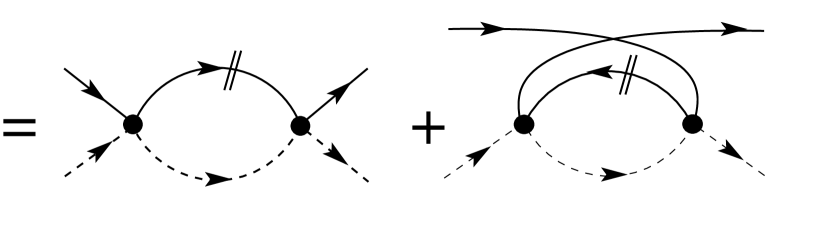
Figure 2: Diagrammatic form of the RG equation (6). The strokes symbolize derivatives with respect to $\ln D$ and $\alpha,\alpha^{\prime}=L/R$, $\sigma,\sigma^{\prime}=\uparrow\!\!\!/\!\!\downarrow$ and $\gamma,\gamma^{\prime}=\uparrow\!\!/\!\!\downarrow$ denote the quantum numbers of the incoming and outgoing conduction electrons and pseudo fermions, respectively. Their frequencies are given by $\omega_{c},\omega_{c}^{\prime},\omega_{f},\omega_{f}^{\prime}$ with $\omega_{c}+\omega_{f}=\omega_{c}^{\prime}+\omega_{f}^{\prime}$.

All leading logarithmic terms in perturbation theory stem from the simple vertex renormalizations shown in Fig. 2 when the real part $\approx 1/(\omega\pm B/2)$ of the pseudo fermion Green function is convoluted with the Keldysh component of the electron line $-2\pi iN_{0}\tanh[(\omega-\mu_{\alpha})/2T]$. Using cutoffs symmetric with respect to $\mu_{L,R}$, respectively, one obtains at $T=0$

$$\frac{\partial}{\partial\ln D}\int_{-D}^{D}d\omega\frac{\text{sign}\ \omega}{\omega-\Delta\omega}\approx 2\Theta(D-|\Delta\omega|)$$ (5)

where $\Delta\omega$ depends on $V$, $B$ and the incoming and outgoing frequencies. Approximating the logarithmic derivative by a Heaviside step function is valid in the two limits $|\Delta\omega|\gg D$ and $|\Delta\omega|\ll D$. To leading order in our small parameter $1/\ln[\max(V,B)/T_{K}]$, the detailed behavior at $|\Delta\omega|\sim D$ is not important. Similarly, it is sufficient to keep track only of the real parts of the coupling constants on one Keldysh contour denoted by $g^{\alpha\sigma\omega_{c};\alpha^{\prime}\sigma^{\prime}\omega_{c}^{\prime}}_{\gamma\omega_{f};\gamma^{\prime}\omega_{f}^{\prime}}$ for an incoming electron in lead $\alpha=L,R$ with energy $\omega_{c}$ and spin $\sigma=\uparrow,\downarrow$ interacting with a pseudo Fermion with spin $\gamma$ and frequency $\omega_{f}$ describing the local spin (see Fig. 2). Primed quantities refer to outgoing particles. A calculation to higher order in $1/\ln[V/T_{K}]$ also has to take into account the imaginary parts and the full Keldysh structure of the vertices which can be neglected here.

From Fig. 2 and Eq. (5) we obtain

$$\frac{\partial g^{\alpha\sigma,\omega_{c};\alpha^{\prime}\sigma^{\prime},\omega_{c}^{\prime}}_{\gamma,\omega_{f};\gamma^{\prime},\omega_{f}^{\prime}}}{\partial\ln D}=\frac{1}{8}\!\sum_{\beta=L,R;\tau,\delta=\uparrow,\downarrow,\lambda=\pm}\biggl{[}\\ \ g^{\alpha\sigma,\omega_{c};\beta\tau,\mu_{\beta}+\lambda D}_{\gamma,\omega_{f};\delta,*}\!g^{\beta\tau,\mu_{\beta}+\lambda D;\alpha^{\prime}\sigma^{\prime},\omega_{c}^{\prime}}_{\delta,*;\gamma^{\prime},\omega_{f}^{\prime}}\,\Theta_{\omega_{c}+\omega_{f}-\mu_{\beta}+\delta B/2}\\ -\ g^{\alpha\sigma,\omega_{c};\beta\tau,\mu_{\beta}+\lambda D}_{\delta,*;\gamma^{\prime},\omega_{f}^{\prime}}\!g^{\beta\tau,\mu_{\beta}+\lambda D;\alpha^{\prime}\sigma^{\prime},\omega_{c}^{\prime}}_{\gamma,\omega_{f};\delta,*}\,\Theta_{\omega_{f}^{\prime}-\omega_{c}+\mu_{\beta}+\delta B/2}\biggr{]}$$ (6)

where

$$\Theta_{\omega}=\Theta(D-|\omega|).$$ (7)

To simplify the notation, “$*$” represents in each term the one frequency, which is fixed by energy conservation. The initial conditions for Eqs. (6) at the bare cutoff are $g^{\alpha\sigma\omega_{c};\alpha^{\prime}\sigma^{\prime}\omega_{c}^{\prime}}_{\gamma\omega_{f};\gamma^{\prime}\omega_{f}^{\prime}}=N_{0}J_{\alpha\alpha^{\prime}}{\boldsymbol{\tau}}_{\sigma\sigma^{\prime}}{\boldsymbol{\tau}}_{\gamma\gamma^{\prime}}$.

The renormalization group equations (6) are rather complex and difficult to solve as each vertex depends on three frequencies. Fortunately, one can drastically simplify them to leading order in $1/\ln[\max(V,B)/T_{K}]$ using two approximations. First, the energy of the spin is well defined and the pseudo fermion spectral functions therefore strongly peaked at $\omega=\pm B/2$, which allows setting $\omega_{f}$ ($\omega{{}^{\prime}}_{f}$) to $-\gamma\frac{B}{2}$ ($-\gamma{{}^{\prime}}\frac{B}{2}$). Hence, one has to keep track only of a single frequency, the energy of the incoming electron. Second, the coupling functions appearing on the right-hand side of (6) depend only logarithmically on the frequency while the Heaviside step function is strongly frequency dependent. This allows to neglect the frequency dependence of the vertices by approximating $f(\Delta\omega)\Theta(D-|\Delta\omega|)\approx f(0)\Theta(D-|\Delta\omega|)$ on the right-hand side of (6).

It is also useful to introduce a more compact notation, which separates spin-flip processes $g_{\perp}$ from non-flip vertices $g_{\|}$ by defining

$$g^{\alpha\sigma,\omega;\alpha^{\prime}\sigma^{\prime},\omega-\frac{(\gamma-\gamma^{\prime})B}{2}}_{\gamma,-\frac{\gamma B}{2};\gamma^{\prime},-\frac{\gamma^{\prime}B}{2}}=\tau_{\sigma\sigma^{\prime}}^{z}\tau_{\gamma\gamma^{\prime}}^{z}g_{z\sigma}^{\alpha\alpha^{\prime}}(\omega)\\ +(\tau_{\sigma\sigma^{\prime}}^{x}\tau_{\gamma\gamma^{\prime}}^{x}+\tau_{\sigma\sigma^{\prime}}^{y}\tau_{\gamma\gamma^{\prime}}^{y})g_{\perp\sigma}^{\alpha\alpha^{\prime}}(\omega-\gamma\frac{B}{2})$$ (8)

The energy argument in the definition of $g_{\perp}$ has been chosen to simplify the RG equations (see below). It turns out that the property $g^{\uparrow\uparrow}_{\uparrow\uparrow}=-g^{\uparrow\uparrow}_{\downarrow\downarrow}$ is preserved under RG, therefore it is not necessary to keep track of a possible $\gamma$ dependence of $g_{z}$. Using these definitions and the approximations described above one obtains

$$\frac{\partial g^{\alpha\alpha^{\prime}}_{\perp\sigma}(\omega)}{\partial\ln D}=-\frac{1}{2}\!\sum_{\beta=L,R}\biggl{[}\\ g^{\alpha\beta}_{\perp\sigma}(-\frac{\sigma B}{2}-\frac{\beta V}{2})g^{\beta\alpha^{\prime}}_{z,-{\sigma}}(-\frac{\beta V}{2})\Theta_{\omega+\frac{\sigma B}{2}+\frac{\beta V}{2}}\\ +g^{\alpha\beta}_{z\sigma}(-\frac{\beta V}{2})g^{\beta\alpha^{\prime}}_{\perp{\sigma}}(\frac{\sigma B}{2}-\frac{\beta V}{2})\Theta_{\omega-\frac{\sigma B}{2}+\frac{\beta V}{2}}\biggr{]}$$ (9)

and for the longitudinal component

$$\frac{\partial g^{\alpha\alpha^{\prime}}_{z\sigma}(\omega)}{\partial\ln D}=-\!\sum_{\beta=L,R}\biggl{[}\\ g^{\alpha\beta}_{\perp\sigma}(-\frac{\sigma B}{2}-\frac{\beta V}{2})g^{\beta\alpha^{\prime}}_{\perp,-{\sigma}}(-\frac{\sigma B}{2}-\frac{\beta V}{2})\Theta_{\omega+\sigma B+\frac{\beta V}{2}}\biggr{]}$$ (10)

The initial values of the RG equations are $g^{\alpha\alpha^{\prime}}_{z\sigma}(\omega)=g^{\alpha\alpha^{\prime}}_{\perp\sigma}(\omega)=g^{\alpha\alpha^{\prime}}$.

The equations (9) and (10) together with the results for the dephasing rates and other physical quantities given below are the main result of this paper. In Ref. [43], these equations have been presented for the special case $g^{\alpha\alpha^{\prime}}=const.$ independent of the lead index, where they simplify drastically (see below).

It is useful to discuss the symmetries of Eq. (9) and (10). Due to the hermiticity of the underlying problem one finds

$$g^{\alpha\alpha^{\prime}}_{\perp\sigma}(\omega) = g^{\alpha^{\prime}\alpha}_{\perp,-\sigma}(\omega)$$ (11)

$$g^{\alpha\alpha^{\prime}}_{z\sigma}(\omega) = g^{\alpha^{\prime}\alpha}_{z\sigma}(\omega).$$ (12)

The coupling matrices simplify drastically in certain limits. For example, if the Kondo model is derived from an underlying Anderson model, then only a single channel couples to the dot and the matrix of bare couplings $g^{\alpha\alpha^{\prime}}$ has only a single non-vanishing eigenvalue. This property is conserved under RG as the RG equations have the matrix structure $\partial\hat{g}=\hat{g}\hat{M}\hat{g}$ and therefore one can express the matrices in LR space in terms of a single function $g_{\perp/z}(\omega)$

$$g^{\alpha\alpha^{\prime}}_{\perp/z}(\omega)=2g_{\perp/z}(\omega)\left(\begin{array}[]{c}\cos\phi\\ \sin\phi\end{array}\right)(\cos\phi,\sin\phi)$$ (15)

Due to (11), $g_{\perp}$ does not depend on $\sigma$ in this case, $g_{\perp\uparrow}(\omega)=g_{\perp\downarrow}(\omega)=g_{\perp}(\omega)$.

In equilibrium, $V=0$, it is well known that within one-loop RG, the two eigenvalues of the coupling constant matrix $\hat{g}=g^{\alpha\alpha^{\prime}}$ do not mix. This is therefore also a property of the RG equations (9) and (10), which have in this case the matrix structure $\partial\hat{g}\propto\hat{g}\hat{g}$. For each of the eigenvalues of $\hat{g}$ one obtains for $V=0$

$$\frac{\partial g_{z\sigma}(\omega)}{\partial\ln D} = -2(g_{\perp}(B/2))^{2}\Theta_{\omega+\sigma B}$$ (16)

$$\frac{\partial g_{\perp}(\omega)}{\partial\ln D} = -g_{\perp}(B/2)g_{z}(0)\left[\Theta_{\omega+B/2}+\Theta_{\omega-B/2}\right]$$

In Ref. [61] we used these equations to calculate the spectral functions at large frequencies and magnetic fields. We checked that these equations indeed reproduce the perturbation theory for the T-matrix not only to order $g^{2}\ln[..]$ but also to order $g^{3}\ln^{2}[..]$ as has to be expected from a theory which resums leading logarithmic corrections. Furthermore, we compared[61] our results to spectral functions calculated with numerical renormalization group and found that the relative errors are – again as expected – of order $1/\ln[\max(\omega,B)/T_{K}]$.

For vanishing magnetic field $B$ and spin-rotational invariant bare couplings $J$, the renormalized coupling constants obviously do not depend on spin and the RG equations simplify to

$$\frac{\partial g^{\alpha\alpha^{\prime}}(\omega)}{\partial\ln D}=-\sum_{\beta=L,R}g^{\alpha\beta}\!(-\frac{\beta V}{2})\,g^{\beta\alpha^{\prime}}\!(-\frac{\beta V}{2})\Theta_{\omega+\beta V/2}.$$ (18)

If the dot couples symmetrically to the left and right lead, one has

$$g_{\perp/z,\sigma}^{LL}(\omega) = g_{\perp/z,-\sigma}^{RR}(-\omega).$$ (19)

If, furthermore, only a single channel couples symmetrically to the dot, one can use (15) to parameterize the renormalized vertices by just two functions $g_{\perp}(\omega)=g_{\perp}(-\omega)$ and $g_{z\uparrow}(\omega)=g_{z\downarrow}(-\omega)$ which are calculated from the RG equations

$$\frac{\partial g_{z\sigma}(\omega)}{\partial\ln D} = -\sum_{\beta=-1,1}g_{\perp}(\frac{B+\beta V}{2})^{2}\Theta_{\omega+\sigma(B+\beta\frac{V}{2})}$$ (20)

$$\frac{\partial g_{\perp}(\omega)}{\partial\ln D} = -\!\!\!\sum_{\beta,\sigma=-1,1}\!\!\!\frac{g_{\perp}(\frac{\sigma B+\beta V}{2})g_{z\sigma}(\frac{\beta V}{2})}{2}\Theta_{\omega+\frac{\sigma B+\beta V}{2}}$$

This limit has been discussed before in Ref. [43].

How are physical quantities calculated from the renormalized coupling constants? To leading order in our small parameter $1/\ln[\max(V,B,\omega)/T_{K}]$ it turns out that it is sufficient to replace in the 2nd order perturbation theory expressions (or, equivalently, in the golden rule expressions) the bare coupling constants by the appropriate renormalized couplings in the limit $D\to 0$. In each case we have checked this by comparing with perturbation theory to order $g^{3}$, where the first logarithmic correction arises[44]. Experimentally the most relevant quantity is the current

$$I=\frac{2\pi e}{16\hbar}\sum_{\gamma\sigma}\int d\omega\,f^{L}_{\omega}(1-f^{R}_{\omega})n_{\gamma}[g_{z\sigma}^{LR}(\omega)]^{2}\\ +4f^{L}_{\omega}(1-f^{R}_{\omega-\gamma B})n_{\gamma}[g_{\perp,-\gamma}^{LR}(\omega-\frac{\gamma B}{2})]^{2}-(L\leftrightarrow R)$$ (21)

where $f^{L/R}_{\omega}=f(\omega\mp V/2)$ are the Fermi functions in the left and right leads. The spin occupations $n_{\uparrow/\downarrow}$ are calculated from the rate equation

$$\Gamma_{\downarrow\to\uparrow}=\Gamma_{\uparrow\to\downarrow}$$ (22)

[see Eq. (2)] with $n_{\uparrow}+n_{\downarrow}=1$ and

$$\Gamma_{\uparrow\to\downarrow}\! = \!\frac{2\pi}{4\hbar}n_{\uparrow}\sum_{\alpha\alpha^{\prime}}\int\!d\omega\,f^{\alpha}_{\omega}(1-f^{\alpha^{\prime}}_{\omega-B})[g_{\perp\downarrow}^{\alpha\alpha^{\prime}}(\omega-\frac{B}{2})]^{2}$$

$$\Gamma_{\downarrow\to\uparrow}\! = \!\frac{2\pi}{4\hbar}n_{\downarrow}\sum_{\alpha\alpha^{\prime}}\int\!d\omega\,f^{\alpha}_{\omega}(1-f^{\alpha^{\prime}}_{\omega+B})[g_{\perp\uparrow}^{\alpha\alpha^{\prime}}(\omega+\frac{B}{2})]^{2}.$$

A quantity of interest for spintronics applications is the spin-current[67] $I_{\text{spin}}=-\frac{1}{2}(\dot{S}_{Lz}-\dot{S}_{Rz})$, where $S_{L/R,z}$ is the $z$ component of the total spin of the conduction electrons in the left/right lead.

$$I_{\text{spin}}=\frac{\pi}{16\hbar}\sum_{\gamma\sigma\alpha\alpha^{\prime}}\int d\omega\,\sigma\frac{\alpha^{\prime}-\alpha}{2}f^{\alpha}_{\omega}(1-f^{\alpha^{\prime}}_{\omega})n_{\gamma}[g_{z\sigma}^{\alpha\alpha^{\prime}}(\omega)]^{2}\\ +4n_{\gamma}f^{\alpha}_{\omega}(1-f^{\alpha^{\prime}}_{\omega-\gamma B})\frac{\alpha+\alpha^{\prime}}{2}[g_{\perp,-\gamma}^{\alpha\alpha^{\prime}}(\omega-\frac{\gamma B}{2})]^{2}$$ (24)

Spin transport will be discussed in detail elsewhere[68].

As we argued in the introduction, the RG flow will finally be cut off and controlled by the dephasing of coherent spin-flips. Therefore one also has to calculate the dephasing rate $\Gamma=1/T_{2}$ by replacing the bare couplings in the perturbative formula[45] by the renormalized couplings

$$\Gamma=\frac{1}{T_{2}}=\frac{\pi}{8\hbar}\sum_{\gamma\sigma\alpha\alpha^{\prime}}\int d\omega\,f^{\alpha}_{\omega}(1-f^{\alpha^{\prime}}_{\omega})[g_{z\sigma}^{\alpha\alpha^{\prime}}(\omega)]^{2}\\ +f^{\alpha}_{\omega}(1-f^{\alpha^{\prime}}_{\omega-\gamma B})[g_{\perp,-\gamma}^{\alpha\alpha^{\prime}}(\omega-\frac{\gamma B}{2})]^{2}$$ (25)

This formula takes into account a partial cancelation of self-energy and vertex corrections. In a careful analysis of perturbation theory, it was shown in Ref. [45], how decoherence rates cut off logarithmic singularities and therefore stop the renormalization group flow. It turns out [45] that different rates (combinations of $1/T_{1}$ and $1/T_{2}$ in the language of NMR) enter the various logarithms. For the situation discussed in this paper, however, the various relaxation rates differ only by factors of order 1. As the relaxation rates appear only (see below) in arguments of logarithms, $\ln\Gamma/T_{K}$, it is not necessary to keep track of these prefactors to leading order in $1/\ln[\max(V,B,\omega)/T_{K}]$. Hence, we can approximate all relaxation rates by $\Gamma$. To leading order, the effect that the self-energy and vertex corrections cut off all logarithmic contributions at the scale $\Gamma$, can be taken into account by replacing

$$\Theta_{\omega}=\Theta(D-\sqrt{\omega^{2}+\Gamma^{2}})$$ (26)

in (9,10). A further effect of the relaxation rate is that spectral functions and spin-spin correlation functions are broadened on the scale $\Gamma$. This can effectively be described by replacing $f_{\omega}$ appearing in (21–25) by Fermi functions smeared out on the scale $\Gamma$ (note, however, that the distribution functions of electrons in the leads are not renormalized). Details of how this broadening is justified and implemented will be published elsewhere[69].

A full solution of the RG equation can now be obtained in the following way (an example is given below): First, the RG equations (9,10) are solved for $\Gamma=0$. This turns out to be rather easy as on the right-hand side of the equations only couplings at a finite set of fixed frequencies enter. One therefore first solves for those frequencies and constructs the full energy dependence in the limit $D\to 0$ in a second step. For some frequencies one will find diverging couplings as the effect of $\Gamma$ has not yet been taken into account. With these frequency dependent couplings, one calculates $\Gamma$ from (25) which is finite as the integrals over the weakly divergent coupling functions do not diverge. With this $\Gamma$ one recalculates the RG equations using (26). In practical numerical implementations, we iterate this procedure until convergence is reached, but formally the effects of self-consistency are subleading and the first iteration described above is sufficient within the precision of our approach. Finally, physical quantities like the magnetization [using (3)], the current (21) or the spectral function [61] are calculated from the renormalized couplings. Note that the approximation, that $\Gamma$ and other physical quantities like the occupations can be calculated in an independent second step after solving the RG equations, is only valid to leading order in $1/\ln[\max(V,B)/T_{K}]$. To higher order, one has to solve simultaneously the RG equations for (frequency dependent) self-energies and vertices.

As an example, we consider a simple situation by calculating the properties of a symmetric dot with $g^{LL}=g^{RR}=g_{d}$ for vanishing magnetic field, $B=0$, and large voltages, $V\gg T_{K}$. From (11) and (19) one finds $g^{LL}(\omega)=g^{RR}(-\omega)=g^{d}(\omega)$ and $g^{LR}(\omega)=g^{RL}(\omega)=g^{LR}(-\omega)$. To solve the RG equations (18), we first observe that on their right hand side only the couplings $g_{d}(V/2)$ and $g^{LR}(V/2)$ enter. Therefore we first determine the RG equation for these two constants

$$\partial g_{d}(V/2) = -[g^{LR}(V/2)^{2}\Theta_{V}+g_{d}(V/2)^{2}\Theta_{\Gamma}]$$

$$\partial g^{LR}(V/2) = -g^{LR}(V/2)g_{d}(V/2)(\Theta_{V}+\Theta_{\Gamma})$$ (27)

with $\Theta_{\Gamma}=\Theta[D-\Gamma]$ and $\Theta_{V}\approx\Theta[D-V]$ as $\Gamma\ll V$. Note, that the RG flow is not completely cutoff by $V$ but continues for $D>\Gamma$. The equations are most conveniently solved in the scaling limit, where the Kondo temperature is held fixed assuming a large initial cutoff $D\to\infty$ and a small bare exchange coupling $J\to 0$. For $D>V$, the RG equations are identical to the RG equations for the two-channel channel-anisotropic Kondo model in equilibrium, the channels are the even (L+R) and odd (L-R) linear combinations of electrons. The RG flow is characterized by two RG invariants, the Kondo temperature $T_{K}=De^{-1/(g_{d}+g^{LR})}$ and $\alpha_{0}=\frac{g_{d}^{2}-(g^{LR})^{2}}{2g^{LR}}$. The RG equations are easily solved and one obtains $g_{d}(V/2)=\frac{1+2\alpha_{0}\ln[D/T_{K}]}{2\ln[D/T_{K}](1+\alpha_{0}\ln[D/T_{K}])}$ for $D>V$ and $g_{d}(V/2)=1/\ln[D/T^{*}]$ with $T^{*}=T_{K}(T_{K}/V)^{1/(1+2\alpha_{0}\ln[V/T_{K}])}$ for $\Gamma<D<V$. The coupling $g_{LR}(V/2)$ is given by $g_{LR}(V/2)=g_{d}(V/2)/(1+2\alpha_{0}\ln[\max(D,V)/T_{K}])$. Plugging these solutions into the right-hand side of (18), one can easily integrate the equations analytically for an arbitrary frequency. As the formulas are rather lengthy, we show only the result for $\alpha_{0}=0$ when only a single channel couples to the dot and $g_{d}(\omega)=g^{LR}(\omega)=g(\omega)$ according to Eq. (15). For $D\to 0$ one finds

$$g(\omega)\approx\sum_{\beta}\Theta[|\omega-\beta V/2|-V]\frac{1}{4\ln[|\omega-\beta V/2|/T_{K}]}\\ +\Theta[V-|\omega-\beta V/2|]\left(\frac{1}{\ln[V\max(|\omega-\beta V/2|,\Gamma)/T_{K}^{2}]}\right.\\ \left.-\frac{1}{4\ln[V/T_{K}]}\right)$$ (28)

where $\Gamma\approx V\frac{\pi}{16\ln[V/T_{K}]^{2}}$ is calculated from (25). In Fig. 2 a plot of $g(\omega)$ is shown for $V/T_{K}=100$, where $\Gamma\approx 1.6T_{K}$. For $V\gg T_{K}$, the relaxation rate is larger than $T_{K}$ and therefore one stays in the weak coupling regime, $g(\omega)\ll 1$ for $\alpha_{0}=0$. As described in detail in Ref. [55], for $\alpha_{0}>1$ the perturbative RG breaks down for large voltages and one enters a strong coupling regime. (In that analysis[55] we did not keep track of the frequency dependent couplings, nevertheless all results remain valid; $g_{LR}$ in Ref. [55] has to be identified with $g_{LR}(\omega=0)$).

Using (28) one can easily calculate physical quantities like the current. As the current is obtained from an integral over $g(\omega)$ it is not sensitive to details of $g(\omega)$ and one finds that the differential conductance is given by $G\approx\frac{3\pi eV}{16\hbar\ln[V/T_{K}]^{2}}$, a result obtained before by Kaminski et al.[28]. A quantity like the susceptibility, however, is sensitive to the peaks in $g(\omega)$ and one finds (restoring the $\alpha_{0}$ dependence) by solving the rate equation (22)

$$\chi(V)=\frac{2}{V}\frac{1+2\alpha_{0}\ln\frac{V}{T_{K}}(1+\alpha_{0}\ln\frac{V}{T_{K}})}{\left(1-\frac{(1+2\alpha_{0}\ln\frac{V}{T_{K}})\ln\left[\ln\frac{V}{T_{K}}(1+\alpha_{0}\ln\frac{V}{T_{K}})\right]}{(1+\alpha_{0}\ln\frac{V}{T_{K}})\ln\frac{V}{T_{K}}}\right)^{2}}$$ (29)

While in the presence of a finite bias voltage, large logarithmic corrections arise [related to the peaks in $g(\omega)$], one obtains in equilibrium to the same order of approximation, just $\chi=1/(2T)$. Expanding this result in the bare couplings, one obtains Eq. (4).

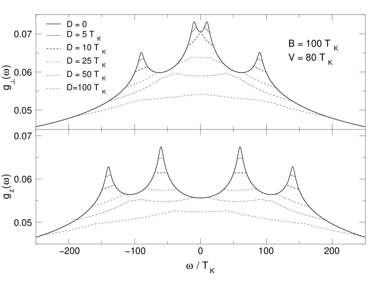
Figure 3: Renormalized coupling constants $g_{\perp}(\omega)$ (upper panel) and $g_{z}(\omega)$ (lower panel) for $B=100T_{K}$ and $V=80T_{K}$ and for different values of the running cut-off $D$. A symmetric dot with bare couplings $g^{\alpha\alpha^{\prime}}=g$ is assumed. Peaks signal that resonant scattering processes take place at those frequencies. The peaks are cutoff by the relaxation rate $\Gamma$.

In Fig. 3, we show the renormalized coupling constants for various values of the running cutoff $D$ in the presence of both a bias voltage $V$ and a magnetic field $B$. While asymptotically the RG equations can be solved analytically, the various crossover regimes have to be calculated from a numerical solution following the approach described above. When the cutoff $D$ is lowered, more and more scattering processes freeze out and only resonant contributions with $\omega\approx\pm V/2\pm B/2$ or $\omega\approx\pm V/2\pm B$ survive and lead to pronounced peaks in the renormalized coupling constants.

Experimentally, the best accessible quantity is the differential conductance $G(V,B)$ as a function of bias voltage and magnetic field. Our calculations can be applied to all systems described by the simple Kondo model (1), e.g. quantum dots with an odd number of electrons in the Coulomb blockade regime, provided that either voltages or magnetic fields are large compared to the Kondo temperature, $V,B\gg T_{K}$, and provided that other excitations of the dot have a much higher energy. The latter requirement is often not fulfilled in quantum dots or molecules. While a generalization of the above described methods to more complex dots and molecules with more levels is straightforward, this will introduce more fitting parameters. If the Kondo model (1) is valid, just two parameters are needed: the Kondo temperature $T_{K}$ and the L/R asymmetry of the coupling $J_{LL}/J_{RR}$ (assuming that only a single channel couples to the Kondo spin as it is the case in most single dot experiments). Both parameters can be determined by comparing the $T$ dependence of the linear-response conductance $G(T,V\to 0,B=0)$ to exact theoretical results determined from numerical renormalization group calculations[70]. This allows for a parameter-free theoretical prediction of $G(V/T_{K},B/T_{K})$ for large $V$ and $B$. In Fig. 4 we compare[43] our theoretical results [determined from a numerical solution of Eqs. (9,10,21,3,25) using (15)] to experiments by Ralph and Buhrman[24], where ratios of $V/T_{K}$ and $B/T_{K}$ larger than 100 have been probed. The peaks in the differential conductance $G(V/B,B/T_{K})$ at $V\sim B$ and their characteristic shape arises due to the interplay of several effects. For $V\ll B$ and $B\gg T_{K}$, the spin is strongly polarized, the Kondo effect is suppressed and transport is dominated by processes where the spin does not flip. For $V\gtrsim B$ a new transport channel is opened, as the voltage provides a sufficient amount of energy to flip the spin. Simultaneously, the magnetization on the dot changes and resonant spin-flip scattering from one Fermi surface to the other strongly renormalizes the effective couplings. The smooth drop at large voltages arises, because the Kondo effect is further suppressed by the voltage. The theory fits the experiment surprisingly well, especially when one takes into account that a relative error of order $1/\ln[\max(V,B)/T_{K}]$ has to be expected from our calculation. Either the next-order correction is accidentally small or some error in the determination of $T_{K}$ (we took the value quoted in the experimental paper[24]) accidentally improves the fit. It is, however, worthwhile to stress, that deviations of theory and experiments are strongest in the regime of small voltages and magnetic fields as expected from an approach based on an expansion in $1/\ln[\max(V,B)/T_{K}]$.

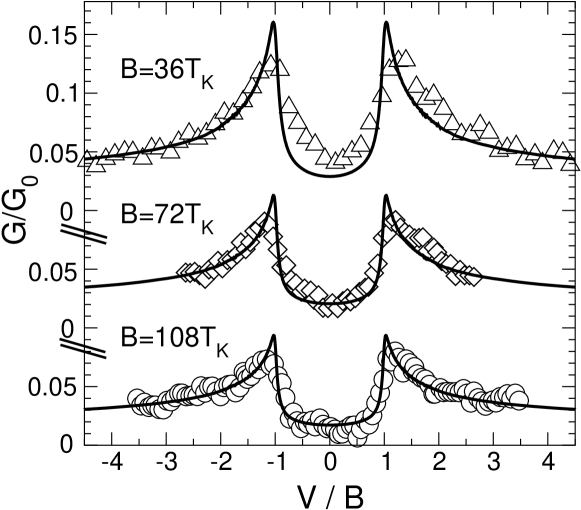
Figure 4: Conductance measurements of Ref. [24] (symbols) on metallic point contacts in magnetic fields $0.85,1.7,2.55\,$T ($B=36,72,104\,T_{K}$, with $T_{K}\approx 30$mK [24]). Assuming that the corresponding point contact is described by a single-channel ($J_{LR}=\sqrt{J_{LL}J_{RR}}$) Kondo model, $\frac{J_{RR}}{J_{LL}}\approx 4.2$ is determined from $G(V\!\!=\!\!0,B\!\!=\!\!0,T\!\!=\!\!50\text{mK})=\frac{4J_{LL}J_{RR}}{(J_{LL}+J_{RR})^{2}}G_{\text{sym}}(T/T_{K})$, where $G_{\text{sym}}$ is known exactly from NRG calculations [70]. This fixes all parameters for our RG calculation (solid lines, $T=0$). As the ($B$-dependent) background is not known experimentally, we subtract $\Delta G=G_{B}-5.2\cdot 10^{-5}G_{0}\frac{V}{T_{K}}$, where $G_{B}$ is fitted to our results at large $V$. The experimental temperature $T=50$mK leads to an extra small broadening at $V=B$. Note that the agreement between theory and experiment is best for large voltages and magnetic fields as expected.

4 Conclusions and Outlook

In the last 40 years the Kondo effect has motivated many new theoretical developments. It can be expected that the Kondo model will also play an important role in developing techniques to understand and describe quantum systems out of equilibrium in regimes where perturbative methods are not available. For example, it would be extremely useful to establish novel numerical methods which are able to calculate e.g. the current-voltage characteristic of a quantum-dot in the Kondo regime. Besides the obvious practical use of methods to predict and explain transport properties of single-electron transistors, molecules and similar systems, we believe that it will be also a conceptual challenge to develop the language and tools to describe and classify strongly interacting quantum systems in steady-state non-equilibrium.

In this paper, we have discussed a simple approach to generalize perturbative renormalization group to a situation, where a finite bias voltage is applied to a quantum dot in the Kondo regime. We derived the one-loop RG equations for a spin coupled to the electrons in two leads by an arbitrary matrix of exchange couplings. This allows a controlled calculation of spectral functions, differential conductances, susceptibilities and other properties of the dot for large bias voltages and/or large magnetic fields and frequencies. The expansion is controlled by the small parameter $1/\ln[\max(V,B,\omega)/T_{K}]$. For the future, it will be interesting to generalize this approach to more complex situations and to investigate systems where the perturbative renormalization group breaks down at large bias voltages[55].

References

- [1] J. Kondo: Prog. Theor. Phys. 32, 37 (1964).
- [2] A. C. Hewson: The Kondo Problem to Heavy Fermions (Cambridge University Press, 1993).
- [3] J. Appelbaum and L. Y. Shen Phys. Rev. B 5, 544 (1972).
- [4] R. H. Wallis and A. F. G. Wyatt: J. Phys. C: Solid State Phys. 7, 1293 (1974).
- [5] E. L. Wolf and D. L. Losee: Phys. Rev. B 2, 3660 (1970).
- [6] L. Y. L. Shen and J. M. Rowell, Phys. Rev. 165, 566 (1968).
- [7] P. Nielsen: Phys. Rev. B 2, 3819 (1970).
- [8] S. Bermon, D. E. Paraskevopoulos and P. M. Tedrow: Phys. Rev. B 17, 210 (1978).
- [9] J. Appelbaum: Phys. Rev. Lett. 17, 91 (1966).
- [10] J. Appelbaum: Phys. Rev. 154, 633 (1967).
- [11] P. W. Anderson: Phys. Rev. Lett. 17, 95 (1966).
- [12] J. Sólyom and A. Zawadowski: Phys. Kondens. Materie 7, 325 (1968); Phys. Kondens. Materie 7, 342 (1968).
- [13] J. Appelbaum and W. F. Brinkman Phys. Rev. B 2, 907 (1970).
- [14] T. Ivezić: J. Phys. C: Solid State Phys., 8, 3371 (1975).
- [15] E. L. Wolf: Principles of Electron Tunneling Spectroscopy, (Oxford University Press, Oxford, 1985).
- [16] D. Goldhaber-Gordon: Hadas Shtrikman: D. Mahalu: David Abusch-Magder: U. Meirav and M. A. Kastner: Nature 391, 156 (1998).
- [17] S. M. Cronenwett, T. H. Oosterkamp and L. P. Kouwenhoven: Science 281, 540 (1998).
- [18] J. Schmid, J. Weis, K. Eberl and K. von Klitzing: Physica B258, 182 (1998).
- [19] J. Nygård, D. H. Cobden and P. E. Lindelof: Nature 408, 342 (2000).
- [20] W. G. van der Wiel, S. De Franceschi, T. Fujisawa, J. M. Elzerman, S. Tarucha, and L. P. Kouwenhoven: Science 289, 2105 (2000).
- [21] D. Goldhaber-Gordon, J. Göres, M. A. Kastner, Hadas Shtrikman, D. Mahalu and U. Meirav: Phys. Rev. Lett. 81, 5225 (1998).
- [22] L. Glazman and M. Raikh: JETP Letters 47, 452 (1988).
- [23] T. Ng and P.A. Lee: Phys. Rev. Lett. 61, 1768 (1988).
- [24] D. C. Ralph and R. A. Buhrman, Phys. Rev. Lett. 72, 3401 (1994).
- [25] S. De Franceschi, R. Hanson, W. G. van der Wiel, J. M. Elzerman, J. J. Wijpkema, T. Fujisawa, S. Tarucha, and L. P. Kouwenhoven: Phys. Rev. Lett. 89, 156801 (2002).
- [26] Y. Goldin and Y. Avishai: Phys. Rev. Lett. 81, 5394 (1998); Phys. Rev. B 61, 16750 (2000).
- [27] J. Appelbaum, J. C. Phillips and G. Tzouras: Phys. Rev. 160, 554 (1967).
- [28] A. Kaminski, Yu. V. Nazarov and L. I. Glazman: Phys. Rev. Lett 83, 384 (1999); Phys. Rev. B 62, 8154 (2000).
- [29] M. H. Hettler and H. Schoeller: Phys. Rev. Lett. 74, 4907 (1995).
- [30] T-K. Ng: Phys. Rev. Lett. 76, 487 (1996).
- [31] R. Lopez, R. Aguado, G. Platero, and C. Tejedor: Phys. Rev. Lett. 81, 4688 (1998).
- [32] A. Kogan, S. Amasha, and M. A. Kastner: Science 304 1293 (2004).
- [33] H. Pothier, S. Guéron, Norman. O. Birge, D. Esteve, and M. H. Devoret, Phys. Rev. Lett. 79, 3490 (1997).
- [34] A. Anthore, F. Pierre, H. Pothier, and D. Esteve, Phys. Rev. Lett. 90, 076806 (2003).
- [35] F. Schopf, C. Bäuerle, W. Rabaud, and L. Saminadayar, Phys. Rev. Lett. 90, 056801 (2003).
- [36] A. Kaminski and L.I. Glazman, Phys. Rev. Lett. 86, 2400 (2001).
- [37] G. Göppert, H. Grabert, Phys. Rev. B 64, 033301 (2001).
- [38] J. Kroha and A. Zawadowski, Phys. Rev. Lett. 88, 176803 (2002).
- [39] N. Sivan and N. S. Wingreen: Phys. Rev. B 54, 11622 (1996).
- [40] S. Hershfield, J. D. Davies, and J. W. Wilkins: Phys. Rev. Lett. 67, 3720 (1991).
- [41] T. Fujii and K. Ueda: Phys. Rev. B 68 (2003) 531.
- [42] A. Oguri: J. Phys. Soc. J. 71 (2002) 2969.
- [43] A. Rosch, J. Paaske, J. Kroha and P. Wölfle: Phys. Rev. Lett. 90, 076804 (2003)
- [44] J. Paaske, A. Rosch, P. Wölfle: Phys. Rev. B 69, 155330 (2004).
- [45] J. Paaske, A. Rosch, J. Kroha, and P. Wölfle: Phys. Rev. B. 70, 155301 (2004).
- [46] O. Parcollet and C. Hooley: Phys. Rev. B 66, 085315 (2002).
- [47] Y. Meir, N. S. Wingreen and P. A. Lee: Phys. Rev. Lett. 70, 2601 (1993).
- [48] N.S. Wingreen and Y. Meir: Phys. Rev. B 49, 11040 (1994).
- [49] M. H. Hettler, J. Kroha and S. Hershfield: Phys. Rev. Lett. 73, 1967 (1994); Phys. Rev. B 58, 5649 (1998).
- [50] J. König, J. Schmid, H. Schoeller and G. Schön, Phys. Rev. B 54, 16820 (1996).
- [51] P. Nordlander, M. Pustilnik, Y. Meir, N. S. Wingreen and D. C. Langreth: Phys. Rev. Lett. 83, 808 (1999);
- [52] M. Plihal, D. C. Langreth, P. Nordlander: Phys. Rev. B 61, R13341 (2000);
- [53] A. Schiller and S. Hershfield, Phys. Rev. B 62, R16271 (2000).
- [54] M. Krawiec and K. I. Wysokinski Phys. Rev. B 66, 165408 (2002)
- [55] A. Rosch, J. Kroha and P. Wölfle: Phys. Rev. Lett. 87, 156802 (2001).
- [56] A. Schiller and S. Hershfield: Phys. Rev. B 51, 12896 (1995); ibid. 58, 14978 (1998); K. Majumdar, A. Schiller and S. Hershfield: Phys. Rev. B 57, 2991 (1998): Yu-Wen Lee and Yu-Li Lee: Phys. Rev. B 65, 155324 (2002).
- [57] R. Aguado and D. C. Langreth: Phys. Rev. Lett. 85, 1946 (2000).
- [58] P. Coleman, C. Hooley, Y. Avishai, Y. Goldin, A. F. Ho: J. Phys.: Condens. Matter 14, L205-L211, (2002).
- [59] J. H. Han, preprint cond-mat/0312023.
- [60] R. M. Konik, H. Saleur and A. Ludwig: Phys. Rev. Lett. 87, 236801 (2001); Phys. Rev. B 66, 125304 (2002).
- [61] A. Rosch, T. A. Costi, J. Paaske, P. Wölfle, Phys. Rev. B 68, 014430 (2003).
- [62] P. W. Anderson: J. Phys. C 3, 2436 (1970).
- [63] N.S. Wingreen, Y. Meir, Phys. Rev. B49, 11040 (1994).
- [64] J. Rammer and H. Smith, Rev. Mod. Phys. 58: 323 (1986).
- [65] M. Salmhofer and C. Honerkamp, Prog. Theo. Physics 105, 1 (2001).
- [66] H. Schoeller and J. König, Phys. Rev. Lett. 84, 3686 (2000); see also M. Keil, Ph.D. thesis, U. Göttingen (2002).
- [67] G. Sellier: Quantum Impurities in Superconductors and Nanostructures: Selfconsistent Approximations and Renormalization Group Analysis, dissertation, University of Karlsruhe, (Shaker, Aachen, 2003).
- [68] G. Sellier, J. Kroha, and A. Rosch: in preparation.
- [69] A. Rosch, J. Paaske and P. Wölfle: in preparation.
- [70] T. A. Costi and A. C. Hewson, J. Phys. Cond. Mat 6, 2519 (1994).