The Effects of Next-Nearest-Neighbor Interactions on the Orientation Dependence of Step Stiffness: Reconciling Theory with Experiment for Cu(001)

Abstract

Within the solid-on-solid (SOS) approximation, we carry out a calculation of the orientational dependence of the step stiffness on a square lattice with nearest and next-nearest neighbor interactions. At low temperature our result reduces to a simple, transparent expression. The effect of the strongest trio (three-site, non pairwise) interaction can easily be incorporated by modifying the interpretation of the two pairwise energies. The work is motivated by a calculation based on nearest neighbors that underestimates the stiffness by a factor of 4 in directions away from close-packed directions, and a subsequent estimate of the stiffness in the two high-symmetry directions alone that suggested that inclusion of next-nearest-neighbor attractions could fully explain the discrepancy. As in these earlier papers, the discussion focuses on Cu(001).

I Introduction

At the nano-scale, steps play a crucial role in the dynamics of surfaces. Understanding step behavior is therefore essential before nano-structures can be self-assembled and controlled. In turn, step stiffness plays a central role in our understanding of how steps respond to fluctuations and driving forces. It is one of the three parameters of the step-continuum model,JW which has proved a powerful way to describe step behavior on a coarse-grained level, without recourse to a myriad of microscopic energies and rates. As the inertial term, stiffness determines how a step responds to interactions with other steps, to atomistic mass-transport processes, and to external driving forces. Accordingly, a thorough understanding of stiffness and its consequences is crucial.

The step stiffness $\tilde{\beta}$ weights deviations from straightness in the step Hamiltonian. Thus, it varies inversely with the step diffusivity, which measures the degree of wandering of a step perpendicular to its mean direction. This diffusivity can be readily written down in terms of the energies $\varepsilon_{k}$ of kinks along steps with a mean orientation along close-packed directions ($\langle 110\rangle$ for an fcc (001) surface): in this case, all kinks are thermally excited. Conversely, experimental measurements of the low-temperature diffusivity (via the scale factor of the spatial correlation function) can be used to deduce the kink energy. A more subtle question is how this stiffness depends on the azimuthal misorientation angle, conventionally called $\theta$ and measured from the close-packed direction. In contrast to $\theta=0$ steps, even for temperatures much below $\varepsilon_{k}$, there are always a non-vanishing number of kinks, the density of which are fixed by geometry (and so are proportional to $\tan\theta$). In a bond-counting model, the energetic portion of the step free energy per length (or, equivalently, the line tension, since the surface is maintained at constant [zero] chargeIS ) $\beta(\theta)$ is cancelled by its second derivative with respect to $\theta$, so that the stiffness is due to the entropy contribution alone. Away from close-packed directions, this entropy can be determined by simple combinatoric factors at low temperature $T$.rottman ; avron ; Cahn

Interest in this whole issue has been piqued by the recent finding by Dieluweit et al. dieluweit02 that the stiffness as predicted in the above fashion, assuming that only nearest-neighbor (NN) interactions $\epsilon_{1}$ are important, underestimates the values for Cu(001) derived from two independent types of experiments: direct measurement of the diffusivity on vicinal Cu surfaces with various tilts and examination of the shape of (single-layer) islands. The agreement of the two types of measurements assures that the underestimate is not an anomaly due to step-step interactions. In that work, the effect of next-nearest-neighbor (NNN) interactions $\epsilon_{2}$ was crudely estimated by examining a general formula obtained by Akutsu and Akutsu,AA showing a correction of order $\exp(-\epsilon_{2}/k_{B}T)$, which was glibly deemed to be insignificant. In subsequent work the Twente group ZP1 considered steps in just the two principal directions and showed that if one included an attractive NNN interaction, one could evaluate the step free energies and obtain a ratio consistent with the experimental results in Ref. dieluweit02, . This group later extended their calculationsZP2 to examine the stiffness.

To make contact with experiment, one typically first gauges the diffusivity along a close-packed direction and from it extracts the ratio of the elementary kink energy $\varepsilon_{k}$ to $T$. Arguably the least ambiguous way to relate $\varepsilon_{k}$ to bonds in a lattice gas model is to extract an atom from the edge and place it alongside the step well away from the new unit indentation, thereby creating four kinks.nelson The removal of the step atom costs energy $3\epsilon_{1}\!+\!2\epsilon_{2}$ while its replacement next to the step recoups $\epsilon_{1}\!+\!2\epsilon_{2}$. Thus, whether or not there are NNN interactions, we identify $\varepsilon_{k}\!=\!-\scriptstyle{\frac{1}{2}}\textstyle\epsilon_{1}\!=\!\scriptstyle{\frac{1}{2}}\textstyle|\epsilon_{1}|$ (since the formation of Cu islands implies $\epsilon_{1}\!<\!0$); thus, as necessary, $\varepsilon_{k}\!>\!0$. Note that for clarity we reserve the character $\epsilon$ for lattice-gas energies,LG which are deduced by fitting this model to energies which can be measured, such as $\varepsilon_{k}$.

The goal of this paper is to compute the step line tension $\beta$ and the stiffness $\tilde{\beta}$ as functions of azimuthal misorientation $\theta$, when NNN (in addition to NN) interactions contribute. Since it is difficult to generalize the low-temperature expansion of the Ising model,rottman ; avron we instead study the SOS (solid-on-solid) model, which behaves very similarly at low temperatures and at azimuthal misorientations that are not too large, but can be analyzed exactly even with NNN interactions. This derivation is described in Section II, with most of the calculational details placed in the Appendix. In Section III we derive a simple expression for the stiffness in the low-temperature limit, presented in Eq. (14). We also make contact with parameters relevant to Cu(001), for which this limit is appropriate. In Section IV we extend the formalism to encompass the presumably-strongest trio (3-atom, non-pairwise) interaction, showing that its effect can be taken into account by shifting the pair energies in the preceding work. The final section offers discussion and conclusions.

II NNN SOS Model on a Square Lattice

Including NNN interactions in the low-temperature expansion of the square-lattice Ising model lifts the remarkable degeneracy of the model with just NN bonds. In that simple case, the energy of a path depends solely on the number of NN links, independent of the arrangement of kinks along it; thus, the energy of the ground state is proportional to the number of NN links of the shortest path between two points, and the entropy is related to the number of combinations of horizontal and vertical links that can connect the points.rottman ; Cahn Including NNN interactions causes the step energy to become a function of both the length of the step and the number of its kinks, eliminating the simple path-counting result.Cahn It can then become energetically favorable for the step to lengthen rather than add another kink. This causes the NN energy levels to split in a non-trivial way, making it possible for a longer step to have a lower energy than a shorter step. A related complication is that the expansion itself depends on the relative strength of the NNN-interaction: Instead of an expansion just in terms of $\exp(-|\epsilon_{1}|/k_{B}T)$, the expansion also is in terms of $\exp(\epsilon_{2}/2k_{B}T)$. Hence, to take the NNN-expansion to the same order of magnitude as the NN-expansion, an unspecified number of terms is required, depending on the size of the ratio $\epsilon_{2}/\epsilon_{1}$.

Since the NNN Ising model cannot be solved exactly and we cannot generalize the low-$T$ expansion, we turn to an SOS model, which was used in earlier examinations of step problems, most notably in the seminal work of Burton, Cabrera, and Frank,BCF and later used for steps of arbitrary orientation by Leamy, Gilmer, and Jackson.Leamy It was also applied to an interface of arbitrary orientation in a square-lattice Ising model.Burk

Although the SOS model can be treated exactly, the result is somewhat unwieldy. Fortunately, at low temperature—the appropriate regime for the experiments under consideration—the solution reduces to a simple expression.

II.1 Description of Model

Consider a step edge of projected length $L$ separating an upper adatom-free region from a lower adatom-filled region (see Fig. 1).

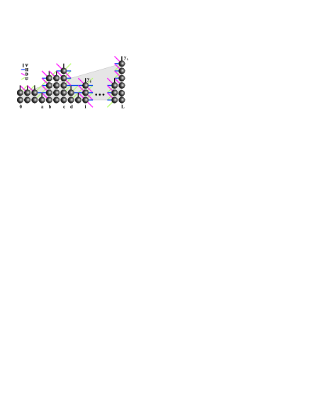
Figure 1: A finite-sized step edge whose projected length is $L$. The step has height $y_{i}$ at position $i$ ($0\leq i\leq L$). The height difference $y_{L}-y_{0}$ is fixed; thus, the step edge makes an angle $\theta$ with the horizontal axis, and has an overall slope $m$ (shown as the top of the gray region). The energy of the step edge is found by counting the number of broken links required to form it. Here all NN and NNN broken links are shown.

The step edge is completely described by specifying its height $y_{i}$ at position $i$ ($0\leq i\leq L$). The energy of the step edge depends on the number of broken bonds required to form it. Let $V$ and $H$ represent the vertical and horizontal NN bond strengths divided by $k_{B}T$, and let $U$ and $D$ represent up-diagonal and down-diagonal NNN bond strengths over $k_{B}T$. Then the step-edge energy $E\equiv E(\{\Delta_{i}\})$ depends only on $\Delta_{i}\equiv y_{i}-y_{i-1}$.

For clarity, we consider two examples. First, if $\Delta_{i}=3$ (as is the case between columns a and b in Fig. 1), then between positions $i$ and $i+1$ there are $3$ broken $H$-links, $2$ broken $U$-links, and $4$ broken $D$-links. There are also $2$ broken $V$-links, but this number is independent of $\Delta_{i}$, since every step-edge configuration of projected length $L$ requires exactly $L$ broken $V$-links. Similarly, if $\Delta_{i}=-3$ (as is the case between columns c and d in Fig. 1), then there would be the same number of broken $H$-links, but there would now be $4$ broken $U$-links and $2$ broken $D$-links (that is, the number of broken $U$ and $D$ links switch from the previous case). From these examples we see that, in general, there are $\left|\Delta_{i}\right|$ broken $H$-links, $\left|\Delta_{i}-1\right|$ broken $U$-links, and $\left|\Delta_{i}+1\right|$ broken $D$-links. It therefore follows that the step-edge energy is

$$\frac{E(\{\Delta_{i}\})}{k_{B}T} = \sum_{i=1}^{L}\Big{(}V+H\left|\Delta_{i}\right|+U\left|\Delta_{i}\!-\!1\right|+D\left|\Delta_{i}\!+\!1\right|\Big{)}$$ (1)

$$\equiv \sum_{i=1}^{L}K(\Delta_{i}).$$

Because we seek the orientation dependence of $\beta$ and $\tilde{\beta}$, we constrain the step to have an overall offset $Y\equiv y_{L}-y_{0}\equiv L\tan\theta=\sum_{i=1}^{L}\Delta_{i}$. (This constraint is represented in Fig. 1 by the shaded gray area. Equivalently, we specify that the overall slope of the step is $m\equiv\tan\theta$.) The constrained partition function is therefore

$$Z\left(Y\right)\equiv\sum_{\left\{\Delta\right\}}\delta\left[Y-\sum_{i=1}^{L}\Delta_{i}\right]e^{-E(\{\Delta_{i}\})/k_{B}T},$$ (2)

where $\{\Delta\}$ is the set of all $\Delta_{i}$ each of which ranges over all integers. From $Z(Y)$ we can find the orientation dependence of the free energy $F(Y)=-k_{B}T\ln Z(Y)$, the projected free energy per length $f(m)=F(Y)/L$, and the line tension (or free energy per length) $\beta(\theta)=f(m)\cos\theta$ (since the step length is $L/\cos\theta$); thence, we can find the stiffness $\tilde{\beta}(\theta)=\beta(\theta)+\partial^{2}\beta(\theta)/\partial\theta^{2}$.

For future reference, note that the process of extracting an atom from the step-edge and replacing it alongside the edge, discussed in the penultimate paragraph of the introduction, creates two pairs of $\Delta\!=\!+1$ and $\Delta\!=\!-1$, costing $4H$ according to Eq. (1) and removing a net of 2 NN bonds, so that $H\!=\!-\epsilon_{1}/2k_{B}T\!=\!\varepsilon_{k}/k_{B}T$. Similarly, we compare the energies of two NN atoms, abutting [the lower side of] a step edge ($\{\Delta_{i}\}\!=\!0$) at $i_{0}$ and either parallel or perpendicular to the edge. In the first case, $\Delta_{i_{0}}\!=\!+1$ and $\Delta_{i_{0}+2}\!=\!-1$, with an added energy of $2H+2(U\!+\!D)$ according to Eq. (1). In the perpendicular case $\Delta_{i_{0}}\!=\!+2$ and $\Delta_{i_{0}+1}\!=\!-2$, implying an added energy of $4H+4(U\!+\!D)$. Counting bonds we see that the parallel configuration has one more $\epsilon_{1}$ bond and two more $\epsilon_{2}$ bonds than the perpendicular configuration. Invoking $H\!=\!-\epsilon_{1}/2k_{B}T$, we see that $U\!+\!D\!=\!-\epsilon_{2}/k_{B}T$; if $U\!=\!D$, then $D\!=\!-\epsilon_{2}/2k_{B}T$. The factor-of-2 difference between broken links in Eq. (1) and broken bonds was noted (for H links) already in the classic exposition by Leamy et al.Leamy An alternate argument, presented over a decade ago,ZELD for this factor of 2 is that the ragged edge is created by severing bonds along the selected path through an infinite square. This leads to the formation of two complementary irregular boundary layers (with opposite values of $\{\Delta_{i}\}$, so that the associated energy of each is half that of the broken bonds (at least when $U\!=\!D$).

II.2 Evaluation of the Free Energy

As detailed in the first part of the Appendix, the sum in the Fourier transform of $Z(Y)$, which we denote by $W(\mu)$, factorizes. Thus, it can be written as

$$W(\mu)=\exp\left[-Lg(i\mu)/k_{B}T\right],$$

where $g(i\mu)$ is the reduced Gibbs free energy per column. To evaluate the inverse transform, we exploit the saddle point method and obtain (see Appendix for details)

$$Z(Y)\approx\exp\left[-L\left(\rho_{0}\tan\theta+\frac{g(\rho_{0})}{k_{B}T}\right)\right],$$ (3)

where the saddle point ($\mu_{0}=$ $-i\rho_{0}$) is defined implicitly by the stationarity condition

$$-\frac{g^{\prime}(\rho_{0})}{k_{B}T}=m\equiv\tan\theta.$$ (4)

Here, prime (as in $g^{\prime}$) denotes a derivative with respect to $\rho$. This result can be regarded as applying a “torque” to the step to produce a rotation $\theta=\tan^{-1}m$ from the minimum-energy, close-packed orientation.Leamy

Taking the logarithm of Eq. (3), we find the projected free energy per column $f(m)$ as a Legendre transform of the reduced Gibbs free energy per column $g(\rho_{0})$:

$$\frac{f(m)}{k_{B}T}\approx\rho_{0}m+\frac{g(\rho_{0})}{k_{B}T}.$$ (5)

Note that this expression is valid only for $L\gg 1$; for finite-sized systems, corrections are required. As standard for Legendre transforms,KSK we have

$$\frac{\ddot{f}(m)}{k_{B}T}=-\frac{k_{B}T}{g^{\prime\prime}(\rho_{0})},$$ (6)

where $\ddot{f}\equiv\partial^{2}f/\partial m^{2}$. Using $\beta(\theta)a=f(m)\cos\theta$ and $m=\tan\theta$, with $a$ the lattice constant of the square (i.e., the column spacing, which is $(1/\sqrt{2})$ the conventional fcc lattice constant), we can rewrite the stiffness as

$$\tilde{\beta}(\theta)a=\ddot{f}(m)/\cos^{3}\theta,$$ (7)

or, similar to results by Bartelt et al.,BEW

$$\frac{k_{B}T}{\tilde{\beta}(\theta)a}=-\frac{g^{\prime\prime}(\rho_{0})}{k_{B}T}\cos^{3}\theta.$$ (8)

Thus, we only need $g^{\prime\prime}(\rho)$ to find the stiffness as a function of $m$ or $\theta$.

Of course, $\rho_{0}$ in $g^{\prime\prime}$ must be eliminated in favor of $m$ via Eq. (4). The details for the general case are somewhat involved. Here, we simplify to the physically relevant case of $U=D$ and, defining $S\equiv H+U+D=H+2D$, just quote the results:

$$\frac{g^{\prime\prime}\left(\rho_{0}\right)}{k_{B}T}=-m\left[\ \frac{2\sinh\rho_{0}}{C(S,\rho_{0})}+\coth\rho_{0}\right]\ +m^{2}$$ (9)

where $C(S,\rho_{0})\equiv\cosh S-\cosh\rho_{0}$ and $\rho_{0}(m)$ is found by inverting

$$m=\frac{\sinh\rho_{0}\sinh S}{C(S,\rho_{0})\left[\sinh S-C(S,\rho_{0})\left(1-e^{-2D}\right)\right]}.$$ (10)

Some details can be found in the Appendix. Since Eq. (10) is a quartic equation for $\cosh\rho_{0}$ or $e^{\rho_{0}}$, the explicit expression for $\rho_{0}(m)$ is rather opaque. However, at low-temperatures, a simpler formula emerges, as shown in the next section.

III Low-T Solution: Simple Expression

At low temperatures, we find that the appropriate root for $\rho_{0}$ diverges. Then we can write $\cosh\rho_{0}\approx\sinh\rho_{0}\approx e^{\rho_{0}}/2$. Of course, $H\propto 1/T$ so that $\cosh S\approx e^{S}/2$. With these approximations, Eq. (10) becomes quadratic in $e^{\rho_{0}}$:

$$m=\frac{e^{\rho_{0}+S}}{(e^{S}-e^{\rho_{0}})[e^{S}-(e^{S}-e^{\rho_{0}})(1-e^{-2D})]}$$ (11)

Likewise, the expression for $g^{\prime\prime}(\rho_{0})$, Eq. (9), becomes

$$\frac{g^{\prime\prime}\left(\rho_{0}\right)}{k_{B}T} = -m\left[\ \frac{2e^{\rho_{0}}}{(e^{S}-e^{\rho_{0}})}+1\right]\ +m^{2}.$$ (12)

Solving for $e^{\rho_{0}}$ in Eq. (11) and inserting the solution into Eq. (12) gives

$$\frac{g^{\prime\prime}\left(\rho_{0}\right)}{k_{B}T} = -m\sqrt{(1-m)^{2}+4me^{-2D}}.$$ (13)

so that, from Eq. (8), and recalling $D\!=\!-\epsilon_{2}/2k_{B}T$, we arrive at our main result, a simple, algebraic expression for $\tilde{\beta}$ as a function of $m$:

$$\frac{k_{B}T}{\tilde{\beta}a}=\frac{m\sqrt{(1-m)^{2}+4me^{\epsilon_{2}/k_{B}T}}}{(1+m^{2})^{3/2}}.$$ (14)

We examine Eq. (14) in several different limiting cases. When $\epsilon_{2}=0$, this reduces to

$$\frac{k_{B}T}{\tilde{\beta}a}=\frac{m+m^{2}}{\left(1+m^{2}\right)^{3/2}}.$$ (15)

as found in a previous study involving only NN interactions.dieluweit02 Interestingly, at $\theta=45^{\circ}$, Eq. (14) shows a simple dependence on $\epsilon_{2}$, namely,

$$\frac{k_{B}T}{\tilde{\beta}a}=\frac{e^{\epsilon_{2}/2k_{B}T}}{\sqrt{2}}.$$ (16)

Of course, this reduces to the venerable Ising result of $1/\sqrt{2}$ in the absence of NNN interactions ($\epsilon_{2}\!=\!0$).rottman ; Ising45 ; Z00

By considering just the lowest and second lowest energy configurations,ZP1 ; ZP2 Zandvliet et al. obtained the resultZP2 (expressed with our sign convention for $\epsilon_{2}$) for the maximally misoriented case $m\!=\!1$

$$\frac{k_{B}T}{\tilde{\beta}a}=\frac{\sqrt{2}}{1+e^{-\epsilon_{2}/2k_{B}T}},$$ (17)

which has, for the attractive $\epsilon_{2}$ of primary concern here, some qualitative similarities to Eq. (16) (including the value $1/\sqrt{2}$ for $\epsilon_{2}\!=\!0$) but is too small by a factor of 2 for $\epsilon_{2}/2k_{B}T\ll 0$; even the coefficient of the first-order term in an expansion in $\epsilon_{2}/2k_{B}T$ is half the correct value. For the opposite limit of repulsive $\epsilon_{2}$, Eq. (17) levels off (at $\sqrt{2}$), in qualitative disagreement with the actual exponential increase seen in Eq. (16).

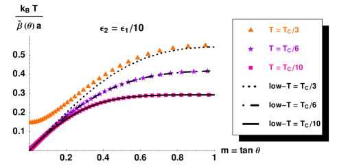
Figure 2: The range of validity of Eq. (14) is examined by comparing it to exact numerical solutions of the SOS model at several temperatures. In the legend $T_{c}$ refers to the NN lattice-gas (Ising) model; for $|\epsilon_{1}|=256$meV, $T_{c}=1685$K.

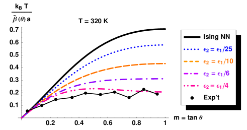
Figure 3: Eq. (14) is plotted for a variety of different values of $D=-\epsilon_{2}/2k_{B}T$, where $\epsilon_{1}$ and $\epsilon_{2}$ are NN- and NNN-interaction energies, respectively, in a lattice-gas picture. The solid curve denoted “Ising NN” corresponds to $\epsilon_{2}\!=\!0$. The dots labeled “Exp’t” are taken from Fig. 2 of Ref. dieluweit02, and were derived from the equilibrium shape of islands on Cu(001) at 302K, with the line segments serving as guides for the eye. To minimize clutter, we omit similar data derived from correlation functions of vicinal surfaces at various temperatures. Note that for $\epsilon_{2}\!=\!\epsilon_{1}/4$ a maximum has developed near $\tan\theta\!=\!1/2$ that is not evident in the experimental data.

Fig. 2 compares Eq. (14) to corresponding exact solutions [found by numerically solving Eqs. (8), (9), and (10)] at several temperatures when $\epsilon_{2}=\epsilon_{1}/10$. We see that Eq. (14) overlaps the exact solution at temperatures as high as $T_{c}/6$. As the temperature increases, the stiffness becomes more isotropic, and Eq. (14) begins to overestimate the stiffness near $\theta=0^{\circ}$.

Finally, in Fig. 3 (using the experimental valueGI $\varepsilon_{k}=128$ meV $\Rightarrow\epsilon_{1}=-256$ meV), we compare Eq. (14) to the NN-Ising model at $T=320$K, as well as to the experimental results of Ref. dieluweit02, . For strongly attractive (negative) $\epsilon_{2}$, $k_{B}T/\tilde{\beta}a$ decreases significantly. In fact, when $\epsilon_{2}/\epsilon_{1}$ is 1/6, so that $-\epsilon_{2}/2k_{B}T=(\epsilon_{2}/\epsilon_{1})(\varepsilon_{k}/k_{B}T)\approx(1/6)4.64$, the model-predicted value of $k_{B}T/\tilde{\beta}a$ has decreased to less than half its $\epsilon_{2}\!=\!0$ value (viz. by a factor of 0.46, vs. 0.63 if Eq. (17) is used), so about 3/2 the experimental ratio. If $\epsilon_{2}/\epsilon_{1}$ increases even further, $k_{B}T/\tilde{\beta}a$ further decreases and develops positive curvature, causing an endpoint local minimum to appear at $\theta=45^{\circ}$. We can determine when this occurs by expanding Eq. (14) about $m=1$:

$$\frac{k_{B}T}{\tilde{\beta}a}=\frac{e^{-D}}{\sqrt{2}}+\left(\frac{e^{D}}{8\sqrt{2}}\!-\!\frac{3e^{-D}}{4\sqrt{2}}\right)(m\!-\!1)^{2}\!+\!\ldots$$ (18)

Setting the coefficient of $(m-1)^{2}$ to zero gives $-2D=\epsilon_{2}/k_{B}T=-\ln(6)\approx-1.8$, which corresponds to a value of $k_{B}T/\tilde{\beta}a=\sqrt{3}/6\approx 0.29$, about 2/5 the value at $\epsilon_{2}\!=\!0$. For $T=320$K and $\varepsilon_{k}=128$ meV, this corresponds to $\epsilon_{2}/\epsilon_{1}\approx 0.2$. However, for the NNN interaction alone to account for the factor-of-4 discrepancy between model/theory and experiment reported by Dieluweit et al.dieluweit02 , Fig. 3 shows that $\epsilon_{2}/\epsilon_{1}\approx 0.3$ would be required.

IV Effect of Trio Interactions

In addition to the NNN interaction, trio (3-atom, non-pairwise) interactions may well influence the stiffness. The strongest such interaction is most likely that associated with 3 atoms forming a right isosceles triangle, whose sides are at NN distance and hypotenuse at NNN separation. In a lattice gas model, there is a new term with $\epsilon_{RT}$ times the occupation numbers of the 3 sites.LG Note that this trio interaction energy $\epsilon_{RT}$ is in addition to the contribution $2\epsilon_{1}\!+\!\epsilon_{2}$ of the constituent pair interactions. If we count broken trios and weight each by $R$, we find an additional contribution to Eq. (1) of $R$ times

$$4|\Delta_{i}|+2\delta_{\Delta_{i},0}+2=2|\Delta_{i}|+|\Delta_{i}\!+\!1|+|\Delta_{i}\!-\!1|+2,$$ (19)

where we have converted the Kronecker delta at $i\!=\!0$ to make better contact with Eq. (1). Thus, without further calculation we can include the effect of this trio by replacing $H$ by $H\!+\!2R$, $U$ by $U\!+\!R$, $D$ by $D\!+\!R$, and (trivially) $V$ by $V\!+\!2$.

By arguments used at the end of Section IIA, we recognize $R\!=\!-\scriptstyle{\frac{1}{2}}\textstyle{\epsilon_{RT}}$. Consequently, the effective NN lattice-gas energy is $\epsilon_{1}\!+\!2\epsilon_{RT}$ and, more significantly the effective NNN interaction energy is $\epsilon_{2}\!+\!\epsilon_{RT}$. Thus, $\epsilon_{RT}$ must be attractive (negative) if it is to help account for the discrepancy in Fig. 2 of Ref. dieluweit02, between the model and experiment. Furthermore, by revisiting the configurations discussed in the penultimate paragraph of the Introduction, we find that the kink energy $\varepsilon_{k}$ becomes $-\scriptstyle{\frac{1}{2}}\textstyle{\epsilon_{1}}-\!\epsilon_{RT}$. Thus, for a repulsive $\epsilon_{RT}$, $|\epsilon_{1}|$ will be larger than predicted by an analysis of, e.g., step-edge diffusivity that neglects $\epsilon_{RT}$. Lastly, the close-packed edge energy, i.e. the $T\!=\!0$ line tension $\beta(0)\!=\!-\scriptstyle{\frac{1}{2}}\textstyle{\epsilon_{1}}-\!\epsilon_{2}$, becomes $-\scriptstyle{\frac{1}{2}}\textstyle{\epsilon_{1}}-\!\epsilon_{2}-\!2\epsilon_{RT}$

V Discussion and Conclusions

We now turn to experimental information about the interactions, followed by comments on the limited available calculations of them, often recapitulating the discussion in Ref. ZP1, . All the experiments are predicated on the belief that at 320K there is sufficient mobility to allow equilibrium to be achieved. If the NNN interactions are to explain at least partially the high stiffness of experiment compared to Ising theory, the NNN interaction must be attractive and a substantial fraction of $\epsilon_{1}$. Since compact islands do form on the Cu(001) surface, it is obvious that $\epsilon_{1}$ is attractive. If $\epsilon_{2}$ is also attractive, as required for reduction of the overestimate of $k_{B}T/\tilde{\beta}$, then the low-temperature equilibrium shape has clipped corners (octagonal-like, with sides of alternating lengths), as noted in Ref. ZP1, ; no evidence of such behavior has been seen. The lack of evidence of a decreasing stiffness near $\theta\approx 45^{\circ}$ suggests that $\epsilon_{2}/\epsilon_{1}$ is at most 1/5.

There is implicit experimental information for $\epsilon_{2}$: from island shapesIsing45 and fluctuationsSGVI $\beta(0)=220\pm\!11\!$ meV. Since related measurements showed $\scriptstyle{\frac{1}{2}}\textstyle{\epsilon_{1}}\!=\!-128$meV, we deduce $\epsilon_{2}\!=\!-92\!$ meV if $\epsilon_{RT}$ is insignificant. These values imply that $\epsilon_{2}/\epsilon_{1}$ is somewhat larger than 1/3, which seems unlikely in light of the unobserved predictions about the shape of islands in that case (cf. the end of Section III).

To corroborate this picture, one should estimate the values of $\epsilon_{1}$ and $\epsilon_{2}$, as well as $\epsilon_{RT}$, from first-principles total-energy calculations. In contrast to Cu(111),Bogi ; Feibel however, no such information even for $\epsilon_{1}$ has been published for Cu(001); there are, however, several semiempirical calculations which found $\varepsilon_{k}\approx 0.14$eV.semi In such calculations based on the embedded atom method (EAM), which work best for late transition and noble fcc metals, the indirect (“through-substrate”) interactions are expected to be strong only when the adatoms share common substrate nearest neighbors; then the interaction should be repulsive and proportional to the number of shared substrate atoms.TLE-Unertl (Longer range pair interactions and multisite non-pairwise interactions are generally very-to-negligibly small in such calculations; they probably underestimate the actual values of these interactions since there is no Fermi surface in this picture, and it is the Fermi wavevector that dominates long-range interactions.) If the NN and NNN interactions on Cu(001) were purely indirect, we would then predict $\epsilon_{2}\!=\!\scriptstyle{\frac{1}{2}}\textstyle{\epsilon_{1}}\!>\!0$. However, whenever direct interactions (due to covalent effects between the nearby adatoms) are important, they overwhelm the indirect interaction. At NN separation, which is the bulk NN spacing, direct interactions must be significant, explaining why $\epsilon_{1}$ can be attractive. It is not obvious from such general arguments whether there are significant direct interactions between Cu adatoms at NNN separations. (For Pt atoms on Pt(100), the only homoepitaxial case in which $\epsilon_{2}$ was computed semiempirically, EAM calculationsWDF gave $\epsilon_{2}/|\epsilon_{1}|$ ​=​ 0.2, less than half the ratio predicted by counting substrate neighbors, but with the predicted repulsive $\epsilon_{2}$.) It is also not obvious a priori whether multi-atom interactions also contribute significantly. (For homoepitaxy, the only semiempirical result is that they are insignificant for Ag on Ag(001);VA however, it is likely that semiempirical calculations will underestimate multi-atom interactions.)

To address these questions, we are currently carrying out calculationsSTK using the VASP package.VASP Preliminary results for Cu(001) suggest that $\epsilon_{2}$ is indeed attractive, and that $\epsilon_{2}/\epsilon_{1}$ is about 1/8; however, there are indications of a repulsive right-triangle trio interaction $\epsilon_{RT}$ with sizable magnitude (perhaps comparable to $|\epsilon_{2}|$, consistent with a priori expectationsTLE-Unertl ; TLE-Maine ), which would diminish rather than enhance the effect of $\epsilon_{2}$.

In summary, NNN interactions may well account for a significant fraction, perhaps even a majority, of the discrepancy between NN Ising model calculations and experimental measurements of the orientation dependence of the reduced stiffness;dieluweit02 the effect is even somewhat greater than estimated by the Twente groupZP1 ; ZP2 . However, inclusion of $\epsilon_{2}$ is not the whole answer, nor, seemingly, is consideration of $\epsilon_{RT}$. One possible missing ingredient is other multi-site interactions, most notably the linear trio $\epsilon_{LT}$ consisting of 3 colinear atoms (a pair of NN legs and an apex angle of $180^{\circ}$). In a model calculation their energy was comparable to $\epsilon_{RT}$,TLE-Unertl ; TLE-Maine albeit with half as many occurrences per atom in the monolayer phase. The corrections due to $\epsilon_{LT}$ would be more complicated than simple shifts in the effective values of $\epsilon_{1}$ and $\epsilon_{2}$. Since direct interactions are probably important, there is no way to escape doing a first-principles computation; we continue to use the VASP package to extend our preliminary calculations.STK A more daunting (at least for lattice-gas afficionadoes) possibility is that long-range intrastep elastic effects may be important. Ciobanu and Shenoy have made noteworthy progress in understanding how this interaction contributes to the orientation dependence of noble-metal steps.shenoy

*

Appendix A Calculational Details

A.1 Partition Function

To carry out the sum in Eq. (2), we consider the Fourier transform of $Z(Y)$:

$$W\left(\mu\right) \equiv \int_{-\infty}^{\infty}dY~{}e^{i\mu Y}Z\left(Y\right)$$ (20)

$$= \sum_{\left\{\Delta\right\}}\exp\sum_{j=1}^{L}\left(i\mu\Delta_{j}-K\left(\Delta_{j}\right)\right)$$

$$= \left[\sum_{\Delta=-\infty}^{\infty}\exp\left(i\mu\Delta-K\left(\Delta\right)\right)\right]^{L},$$

where $K\left(\Delta\right)\equiv\left(V+H\left|\Delta\right|+U\left|\Delta-1\right|+D\left|\Delta+1\right|\right)$ is the energy in Eq. (1), associated with adjacent columns with height difference $\Delta$. Carrying out the summation in Eq. (20) gives

$$\frac{g\left(i\mu\right)}{k_{B}T}\equiv-\frac{1}{L}\ln W(i\mu)=V+U+D-\ln B(i\mu),$$ (21)

where

$$B(i\mu)\equiv 1+\frac{e^{2D}}{e^{H+U+D+i\mu}-1}+\frac{e^{2U}}{e^{H+U+D-i\mu}-1}.$$ (22)

Thus, the original partition function $Z(Y)$ is:

$$Z\left(Y\right) = \frac{1}{2\pi}\int_{-\infty}^{\infty}d\mu~{}e^{-i\mu Y}W\left(\mu\right)$$

$$= \frac{1}{2\pi}\int_{-\infty}^{\infty}d\mu~{}\exp\left[L\left(-i\mu\tan\theta-\frac{g(i\mu)}{k_{B}T}\right)\right]$$

For $L\gg 1$, we can evaluate this inverse transform by steepest decent approximation. The saddle point occurs on the imaginary axis ($\mu=-i\rho$), at the value $\rho_{0}$ given by the stationary-phase condition:

$$-\frac{g^{\prime}\left(\rho_{0}\right)}{k_{B}T}=m\equiv\tan\theta.$$ (24)

Calculating the derivative from Eqs. (21) and (22), we find

$$m=B^{\prime}(\rho_{0})/B(\rho_{0}),$$ (25)

where prime stands for $\partial_{\rho}$. The leading contribution to this integral (A.1) is just the integrand evaluated at this point:

$$Z(Y)\approx\exp\left[-L\left(m\rho_{0}+\frac{g\left(\rho_{0}\right)}{k_{B}T}\right)\right].$$ (26)

A.2 Analysis of $g^{\prime\prime}(\rho)$ and specialization to $U=D$

From Eqs. (21), we find

$$\frac{g^{\prime}\left(\rho\right)}{k_{B}T}=-B^{\prime}(\rho)/B(\rho)$$ (27)

and

$$\frac{g^{\prime\prime}\left(\rho\right)}{k_{B}T}=-B^{\prime\prime}(\rho)/B(\rho)+\left[B^{\prime}(\rho)/B(\rho)\right]^{2}.$$ (28)

This can be simplified, by Eq. (25), to

$$\frac{g^{\prime\prime}\left(\rho_{0}\right)}{k_{B}T}=-mB^{\prime\prime}(\rho_{0})/B^{\prime}(\rho_{0})+m^{2},$$ (29)

the quantity needed for computing the stiffness as a function of $m$. While straightforward, computing the derivatives with the general form for $B$ (Eq. (22) with $\rho=i\mu$) is quite tedious. A slight simplification emerges if we specialize to the physically relevant case $U=D$. Then, with $S\equiv H+2D$, we have

$$B(\rho) = 1+\frac{e^{2D}}{e^{S+\rho}-1}+\frac{e^{2D}}{e^{S-\rho}-1}$$ (30)

$$= 1-e^{2D}+\frac{e^{2D}\sinh S}{\cosh S-\cosh\rho}$$

$$\equiv 1-e^{2D}+\frac{e^{2D}\sinh S}{C(S,\rho)},$$

so that

$$B^{\prime}(\rho)=e^{2D}\sinh S\frac{\sinh\rho}{C^{2}(S,\rho)},$$ (31)

and

$$B^{\prime\prime}(\rho)=e^{2D}\sinh S\left[\frac{\cosh\rho}{C^{2}(S,\rho)}+\frac{2\sinh^{2}\rho}{C^{3}(S,\rho)}\right].$$ (32)

Inserting these expressions into Eq. (25), we have

$$m=\frac{\sinh\rho_{0}\sinh S}{C(S,\rho_{0})\left[\sinh S-C(S,\rho_{0})\left(1-e^{-2D}\right)\right]}.$$ (33)

Similarly, with Eq. (29), we find

$$\frac{g^{\prime\prime}\left(\rho_{0}\right)}{k_{B}T}=-m\left[\ \frac{2\sinh\rho_{0}}{C(S,\rho_{0})}+\coth\rho_{0}\right]\ +m^{2}.$$ (34)

References

- (1) H.-C. Jeong and E. D. Williams, Surf. Sci. Rept. 34, 171 (1999).
- (2) This simple equivalency does not hold for stepped surfaces in an electrochemical system, where the electrode potential is fixed rather than the surface charge density conjugate to . H. Ibach and W. Schmickler, Phys. Rev. Lett. 91, 016106 (2003).
- (3) C. Rottman and M. Wortis, Phys. Rev. B 24, 6274 (1981).
- (4) J.E. Avron, H. van Beijeren, L. S. Schulman, and R. K. P. Zia, J. Phys. A 15, L81 (1982); R.K.P. Zia and J.E. Avron, Phys. Rev. B 25, 2042 (1982).
- (5) J.W. Cahn and R. Kikuchi, J. Phys. Chem. Solids 20, 94 (1961).
- (6) S. Dieluweit, H. Ibach, M. Giesen, and T. L. Einstein, Phys. Rev. B 67, 121410 (2003).
- (7) N. Akutsu and Y. Akutsu, Surf. Sci. 376, 92 (1997).
- (8) N. C. Bartelt, T. L. Einstein, and E. D. Williams, Surf. Sci. 276, 308 (1992).
- (9) R. Van Moere, H. J. W. Zandvliet, and B. Poelsema, Phys. Rev. B 67, 193407 (2003).
- (10) H. J. W. Zandvliet, R. Van Moere, and B. Poelsema, Phys. Rev. B 68, 073404 (2003).
- (11) R. C. Nelson, T. L. Einstein, S. V. Khare, and P. J. Rous, Surf. Sci. 295, 462 (1993).
- (12) Explicitly, the contribution to the lattice-gas Hamiltonian of all NN bonds is , where the site-occupation variable , and the summation is over all NN pairs of sites. It is well known that in the corresponding Ising model, so that is determined by . Unfortunately, the variety of notations in papers on this subject can lead to confusion. In Refs. ZP1, ; ZP2, , have the opposite sign of our . In Ref. Ising45, and somewhat implicitly in Ref. dieluweit02, , the so-called the Ising parameter, , is .
- (13) W. K. Burton, N. Cabrera, and F. C. Frank, Phil. Trans. Roy. Soc. (London) Series A-Math. and Phys. Sci. 243, 299 (1951).
- (14) H. J. Leamy, G. H. Gilmer, and K. A. Jackson, in: Surface Physics of Materials, vol. 1, edited by J. M. Blakely (Academic, New York, 1975), p. 121.
- (15) T. W. Burkhardt, Z. Phys. 29, 129 (1978).
- (16) H. J. W. Zandvliet, H. B. Elswijk, E. J. van Loenen, and D. Dijkkamp, Phys. Rev. B 45, 5965 (1992).
- (17) M. Giesen, C. Steimer, and H. Ibach, Surf. Sci. 471, 80 (2001).
- (18) While this issue is treated in textbooks, a more-readily-accessible exposition of the negative reciprocal relationship between the field and conjugate density susceptibilities is given (in an introductory review couched in magnetic language) by M. Kollar, I. Spremo, and P. Kopietz, Phys. Rev. B 67, 104427 (2003).
- (19) H. J. W. Zandvliet, Phys. Rev. B 61, 9972 (2000).
- (20) M. Giesen-Seibert and H. Ibach, Surf. Sci. 316, 205 (1994); M. Giesen-Seibert, F. Schmitz, R. Jentjens, and H. Ibach, Surf. Sci. 329, 47 (1995).
- (21) C. Steimer, M. Giesen, L. Verheij, and H. Ibach, Phys. Rev. B 64, 085416 (2001).
- (22) A. Bogicevic, S. Ovesson, P. Hyldgaard, B. I. Lundqvist, H. Brune, and D. R. Jennison, Phys. Rev. Lett. 85, 1910 (2000).
- (23) P. J. Feibelman, Phys. Rev. B 60, 11118 (1999).
- (24) Using EAM, C. S. Liu and J. B. Adams, Surf. Sci. 294, 211 (1993) found meV. Using a pair-potential expansion from a first-principles database of surface energies, L. Vitos, H. L. Skriver, and J. Kollár, Surf. Sci. 425, 212 (1999) obtained meV. With an tight-binding model, F. Raouafi, C. Barreteau, M. C. Desjonquères, and D. Spanjaard, Surf. Sci. 505, 183 (2002) calculated meV.
- (25) T. L. Einstein, in: Handbook of Surface Science, edited by W. N. Unertl, Vol. 1 (Elsevier Science B. V., Amsterdam, 1996), ch. 11.
- (26) A. F. Wright, M. S. Daw, and C. Y. Fong, Phys. Rev. B 42, 9409 (1990).
- (27) I. Vattulainen, unpublished, private communication, in conjunction with J. Merikoski, I. Vattulainen, J. Heinonen, and T. Ala-Nissila, Surf. Sci. 387, 167 (1997).
- (28) T. J. Stasevich, T. L. Einstein, and S. Stolbov, in preparation.
- (29) G. Kresse and J. Hafner, Phys. Rev. B 47, 558 (1993); Phys. Rev. B 49, 14 251 (1994); G. Kresse and J. Furthmüller, Comput. Mater. Sci. 6, 15 (1996); Phys. Rev. B 54, 11169 (1996).
- (30) T. L. Einstein, Langmuir 7, 2520 (1991), Surf. Sci. 84, 497 (1979).
- (31) V.B. Shenoy and C.V. Ciobanu, Surf. Sci. 554, 222 (2004).