Piezo-Magneto-Electric Effects in p-Doped Semiconductors

Abstract

We predict the appearance of a uniform magnetization in strained three dimensional p-doped semiconductors with inversion symmetry breaking subject to an external electric field. We compute the magnetization response to the electric field as a function of the direction and magnitude of the applied strain. This effect could be used to manipulate the collective magnetic moment of hole mediated ferromagnetism of magnetically doped semiconductors.

Antiferromagnetic dielectrics with inversion asymmetry exhibit the magnetoelectric (ME) effect, a phenomenon in which a static electric field induces a uniform magnetization landau ; schmidt75 . Moreover, as first pointed out by Levitov et.al. levitov , a kinematic magnetoelectric (kME) effect can also occur in ostensibly nonmagnetic conductors, with spin-orbit coupling, which lack a center of inversion symmetry. Unlike in dielectrics, in the case of conductors, the electric field induced magnetization density, $M_{i}=\alpha_{ij}E_{j}$, is necessarily accompanied by dissipation. Since ${\bf M}$ is odd under time reversal (T) and ${\bf E}$ is even, $\alpha_{ij}$ must be proportional to the relaxation time, a quantity related to the entropy production, making the process dissipative. In addition, since ${\bf M}$ is even under parity (P) while ${\bf E}$ is odd, $\alpha_{ij}$ is zero for parity invariant systems. The kME effect also vanishes in the absence of spin-orbit interaction. In 2D n-doped inversion layers with Rashba spin-orbit interaction, this effect has been predicted more than a decade ago edelstein ; aronov , but has been observed experimentally only very recently kato ; ganichev .

In the model used by Levitov et. al.levitov , the kME effect originates from an electron scattering by impurities whose potential lacks inversion symmetry. As such, the effect is extrinsic and actually vanishes in the clean limit.

In contrast, we present an analysis of hole-doped semiconductor without inversion symmetry where the spin-orbit splitting of the p-band is intrinsic. In the absence of strain the system is both T and P invariant and hence no kME effect occurs. As we argue below, the shear strain induces a P-breaking term in the Hamiltonian which is responsible for the effect.

There are several advantages to having a piezo-magneto-electric effect in 3D p-doped semiconductors (such as GaAs, GaSb, InSb, InGaAs, AlGaAS). Technologically, engineering of different original strain architectures is a common procedure in today’s semiconductor applications. By taking place in a 3D bulk sample, rather than in a 2D sample, this effect allows (with specific strain configurations) full spatial manipulation of the magnetic moment. Most importantly, the effect occurs in p-doped semiconductors, and thus it allows manipulation of the direction of the collective ferromagnetic moment which develops in (p-doped) dilute magnetic semiconductors.

Within the spherical approximation zhang03 ; lut , the effective Hamiltonian of a hole-doped semiconductor with spin-orbit coupling is described by the Luttinger-Kohn model in the spin-$3/2$ band:

$$H_{LK}=\frac{1}{2m}\left(\gamma_{1}+\frac{5}{2}\gamma_{2}\right){\bf k}^{2}-\frac{1}{m}\gamma_{2}({\bf k}\cdot{\bf S})^{2},$$ (1)

where $S_{i}$ is the spin-$3/2$ (4$\times$4 matrix) operator, $\gamma_{1}$ and $\gamma_{2}$ are material-dependent Luttinger constants. The band structure consists of a doubly degenerate heavy hole band corresponding to $\hat{{\bf k}}\cdot{\bf S}=\pm 3/2$ and a doubly degenerate light hole band with $\hat{{\bf k}}\cdot{\bf S}=\pm 1/2$ (see inset of Fig.(1)). The above Hamiltonian is both $P$ and $T$ invariant. The strain, being a second order symmetric tensor $\epsilon_{ij}$, naturally couples to $S_{i}S_{j}$ and to zero-th order modifies the original Hamiltonian $H_{LK}$ by the term

$$H_{\epsilon}=D_{d}(\epsilon_{xx}+\epsilon_{yy}+\epsilon_{zz})+D_{u}\epsilon_{ij}S_{i}S_{j},\;\;\;i,j=x,y,z$$ (2)

where $D_{d}$ and $D_{u}$ are the usual hydrostatic and shear deformation potentials pikus . The modified Hamiltonian $H_{LK}+H_{\epsilon}$ remains invariant under both P and T. Each of the two valence bands is still doubly degenerate. As seen in Fig. (1), the strained Hamiltonian exhibits a finite energy gap between the heavy and light hole bands at zero momentum k=0. External electric field will cause a spin current zhang03 , but no uniform magnetization. For semiconductors with inversion symmetry these are the only terms allowed at quadratic order in ${\bf k}$.

However, in the absence of an inversion symmetry center, the shear strain induces a P-breaking term linear in momentum pikus :

$$H^{\prime}=\lambda_{i}S_{i},\;\;\;\lambda_{x}=C_{4}(\epsilon_{xy}k_{y}-\epsilon_{xz}k_{z}),$$ (3)

where $\lambda_{y},\lambda_{z}$ are obtained from $\lambda_{x}$ by cyclic permutation of indices and $C_{4}$ is a material constant related to the interband-deformation potential for acoustic phonons. This term is responsible for the piezo-kME effect. Its origin can be traced back to the Kane’s $8\times 8$ model ($2\times 2$ for each the conduction and the split-off band, and $4\times 4$ for the valence band)(Fig.(1)), within which the valence band couples to both the conduction band and the split-off band. Upon straining, the zeroth order effect is the P-invariant coupling mentioned in the previous paragraph. At the first order, the conduction band $|s\rangle$ and the valence bands $|x\rangle,|y\rangle,|z\rangle$ couple, and the matrix elements between the valence and conduction band have the form $\epsilon_{xy}\langle s|\partial_{x}\partial_{y}|z\rangle$ (plus cyclic permutations) where $|s\rangle$ is the $s$-orbital and $|z\rangle$ is one of the $p$ orbitals. Any other combination will not satisfy the $L_{z}$ selection rule. In systems with inversion symmetry where the selection rules for L are satisfied, it is impossible to couple the spin-$0$ ($|s\rangle$) conduction states with spin-$1$ ($|x\rangle,|y\rangle,|z\rangle$) valence states through a spin-$2$ term (rank 2 tensor) ($\epsilon_{ij}$) and hence $\langle s|\partial_{x}\partial_{y}|z\rangle=0$. However, when inversion symmetry is broken, $\langle s|\partial_{x}\partial_{y}|z\rangle\neq 0$ as the L selection rule does not apply. We then obtain an $8\times 8$ Kane matrix with the strain terms describing the interaction between valence and conduction bands. To find an effective $4\times 4$ hamiltonian for the valence band, one must project onto the valence band while taking into account the interactions with the conduction and the split-off band. The first term which appears in perturbation theory is the Hamiltonian (3). Reciprocally, a similar term will appear in the conduction band, with the spin there being a spin-1/2 matrix. These terms have been observed experimentally seiler although recent evidence suggests other effects could also play a role kato .

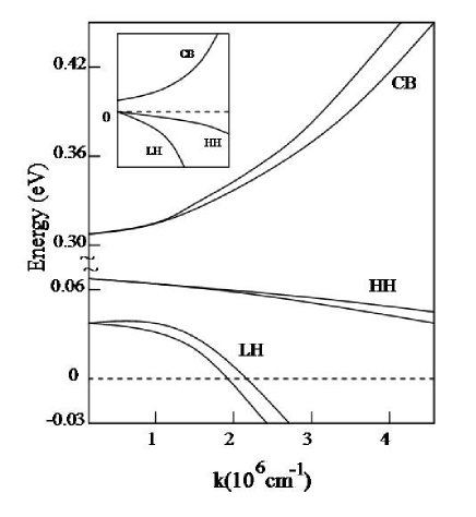
Figure 1: Dispersion curves for InSb at $4$ kbar stress on the $[110]$ direction ($\epsilon_{xy}\approx 2\times 10^{-3}$) and $\vec{k}\parallel[1{\overline{1}}0]$ as measured by Seiler et al seiler . The strain splits the conduction and the valence bands. The Dresselhaus $k^{3}$ type inversion asymmetry is negligibly small on this scale. No splitting is observed for strain in the $[001]$ direction.

The piezo-kME effect can be easily understood as follows: assume a material strained only along the $[110]$ direction, such that $\epsilon_{xy}\neq 0$ is the only nonvanishing shear strain component. Hence, the P-breaking term in the hamiltonian is $H^{\prime}=C_{4}(\epsilon_{xy}k_{y}S_{x}-\epsilon_{yx}k_{x}S_{y})$. This effectively corresponds to Zeeman coupling of hole-spins with a fictitious internal magnetic field $B_{x}=C_{4}\epsilon_{xy}k_{y}/\mu_{B},\;\;B_{y}=-C_{4}\epsilon_{xy}k_{x}/\mu_{B}$, $\mu_{B}$ being the Bohr magneton. Upon the application of an electric field along, say, the $y$ axis, the average momenta become $<k_{x}>\approx 0,\;\;k_{y}\approx eE\tau/m$ where $\tau$ is the momentum relaxation time. In turn, this gives $<B_{y}>\approx 0,\;\;<B_{x}>\approx C_{4}\epsilon_{xy}eE\tau/m\mu_{B}$. The non-zero $<B_{x}>$ field now couples to the spins and orients them along the $x$ axis. This gives rise to a magnetization perpendicular to the electric field. Alternatively, the electric field along the $x$ axis will induce magnetization along the $y$ axis of equal modulus but of opposite sign to the previous one. This has recently been observed in the conduction band by Kato et.al. Ref.kato . Moreover, if we assume linear dependence on the relaxation time, $\tau$, and neglect the effect of parity conserving strain term, then the the form of $\alpha_{ij}$ is constrained by dimensional analysis alone

$$\alpha_{ij}=\mu_{B}n^{\frac{2}{3}}\frac{e\tau}{\hbar}\times\Phi_{ij}\!\!\left(\!\frac{mC_{4}}{\gamma_{1}\hbar^{2}n^{\frac{1}{3}}},\frac{\gamma_{1}}{\gamma_{2}}\!\right),$$ (4)

where $n$ is the carrier density and the scaling function $\Phi_{ij}(x,y)$ vanishes linearly with its first argument $x$. Based on the above argument, up to a sign, its components should be proportional to $\epsilon_{ij}$.

We shall now justify the above claims. The static spin response to the d.c. electric field can be shown to be given by

$$\alpha_{\mu\nu}=\frac{\mu_{B}}{\hbar}\lim_{\omega\rightarrow 0}\Im m\left[\frac{Q^{ret}_{\mu\nu}(\omega)}{\omega}\right],$$ (5)

where $\mu_{B}$ is the Bohr magneton and the retarded correlation function $Q^{ret}_{\mu\nu}(\omega)=Q_{\mu\nu}(i\omega\rightarrow\omega+i\eta)$, ($\eta\rightarrow 0^{+}$), and

$$Q_{\mu\nu}(i\omega)=\int_{0}^{\beta}d\tau e^{i\omega\tau}\langle TS_{\mu}(\tau)j_{\nu}(0)\rangle.$$ (6)

For d.c. response only spatial averages of the spin and the current operators need to be considered above. The corresponding diagram is shown in Fig.(2).

Since the strain splitting is typically small compared to the spin-orbit splitting at the Fermi surface (Fig.1), we can include its effects within (degenerate) perturbation theory. Utilizing the powerful mapping between spin-$3/2$ SU(2) and SO(5) representations pioneered by Murakami, Nagaosa and Zhang zhang03 , the unperturbed thermal Green’s functions can be conveniently written as

$$G_{0}({\bf k},i\omega_{n})=\frac{1}{2}\sum_{s=\pm 1}\frac{1+s\hat{d}_{j}({\bf k})\Gamma_{j}}{-i\omega_{n}+(1+s\Delta)\epsilon({\bf k})},$$ (7)

where $\Delta=2\gamma_{2}/\gamma_{1}$, $\epsilon({\bf k})=\gamma_{1}{\bf k}^{2}/2m$, $j=1,\ldots,5$ and $\hat{d}({\bf k})$ is a (spherical) unit vector in the 5-dimensional space, equivalently $\hat{d}_{m}({\bf k})=Y^{m}_{l=2}(\theta_{{\bf k}},\phi_{{\bf k}})$ where $Y$’s are spherical harmonics and the angles are in ${\bf k}-$space; $\Gamma_{j}$ are 5 Dirac gamma matrices zhang03 . Upon inclusion of spinless impurities with potential $u({\bf k})$, the full (impurity) Green’s function $G({\bf k},i\omega_{n})=G_{0}({\bf k},i\omega_{n}+\Sigma({\bf k},i\omega_{n}))$. Within the Born approximation the self-energy is $\Sigma({\bf k},i\omega_{n})=n_{imp}\int\!\!d{\bf q}\;|u({\bf k}-{\bf q})|^{2}G_{0}({\bf q},i\omega_{n})$; $n_{imp}$ is the concentration of impurities. Finally, to leading order in P breaking strain neglect ,

$${\cal G}({\bf k},i\omega_{n})=\left[1-G({\bf k},i\omega_{n})H^{\prime}({\bf k})\right]G({\bf k},i\omega_{n}).$$ (8)

Subsequently, all of the calculations will be carried out using (8).

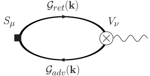
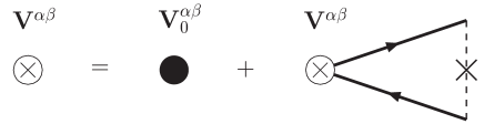
Figure 2: Top: Feynman diagram representing the kinematic Magneto-Electric effect in 3D. Bottom: Kinetic equation for the vertex matrix in the ladder approximation. Here ${\bf V}_{0}^{\alpha\beta}$ is the velocity operator in the absence of impurities.

As shown in Fig.(2), the finite frequency response function (6) is given by

$$Q_{\mu\nu}(i\Omega)=-\frac{e}{\beta}\sum_{\omega_{n}}\int d{\bf k}Tr\left[S_{\mu}\Pi_{\nu}({\bf k},i\omega,i\Omega)\right],$$ (9)

where the trace is over the heavy/light hole spaces and where, as shown in Fig.(2), the ($4\times 4$ matrix) vertex function $\Pi_{\nu}$ satisfies the kinetic equation (within the ladder approximation)

$$\Pi_{\mu}({\bf k},i\omega,i\Omega)={\cal G}({\bf k},i\omega)V_{\nu}({\bf k}){\cal G}({\bf k},i\omega-i\Omega)+n_{imp}{\cal G}({\bf k},i\omega)\int\!\!d{\bf q}|u({\bf k}-{\bf q})|^{2}\Pi_{\nu}({\bf q},i\omega,i\Omega){\cal G}({\bf k},i\omega-i\Omega);$$ (10)

The velocity operator $V_{\mu}({\bf k})=\partial H({\bf k})/\partial k_{\mu}$. Note that ${\cal G}$ does not commute with $\Pi_{\nu}$. As such we have 16 coupled integral equations to solve, one for each entry of the 4$\times$4 matrix. In the case of $\delta$-function impurities $u({\bf k}-{\bf q})=u_{0}$ is a constant and the above integral equation is separable. Integrating both sides over ${\bf k}$, it is easy to see that in the absence of parity breaking strain, the vertex correction vanishes murakami . On the other hand, for finite strain, the vertex correction does not vanish, and we still have to solve a system of 16 coupled equations.

However, to leading order in the strain it can be seen that all 16 equations decouple in the basis of the Clifford algebra! Expanding the vertex matrix

$$\Pi_{\mu}({\bf k},i\omega,i\Omega)=\sum_{A=0}^{15}\lambda_{\mu}^{A}({\bf k},i\omega,i\omega-i\Omega)\Gamma_{A},$$ (11)

where the sum runs over all 16 elements sakurai and $\lambda_{\mu}^{A}({\bf k},i\omega,i\omega-i\Omega)$ is now an ordinary vector function. Since $Tr[\Gamma_{A}\Gamma_{i}\Gamma_{B}\Gamma_{i}]$ is diagonal in $A$ and $B$ it is easy to see that

$$\frac{1}{4}\!\!\int\!\!d{\bf k}Tr[\Gamma_{A}{\cal G}({\bf k},i\omega)\Gamma_{B}{\cal G}({\bf k},i\omega-i\Omega)]=M_{A}(i\omega,i\Omega)\delta_{AB}$$

Therefore,

$$\Pi_{\mu}({\bf k},i\omega,i\Omega)\!\!=\!\!{\cal G}({\bf k},i\omega)\bigl{(}V_{\mu}({\bf k})\!+\!R_{\mu}(i\omega,i\Omega)\bigr{)}{\cal G}({\bf k},i\omega\!-\!i\Omega).$$ (12)

where

$$R_{\mu}(i\omega,i\Omega)=n_{imp}u_{0}^{2}\left(\sum_{A=0}^{15}\frac{\Gamma_{A}V^{A}_{\mu}(i\omega,i\Omega)}{1-n_{imp}u_{0}^{2}M_{A}(i\omega,i\Omega)}\right)$$ (13)

and

$$V^{A}_{\mu}(i\omega,i\Omega)=\frac{1}{4}\!\!\int\!\!d{\bf k}Tr\left[\Gamma_{A}{\cal G}({\bf k},i\omega)V_{\mu}({\bf k}){\cal G}({\bf k},i\omega-i\Omega)\right],$$ (14)

$$M_{A}(i\omega,i\Omega)=\frac{1}{4}\!\!\int\!\!d{\bf k}Tr\left[\Gamma_{A}{\cal G}({\bf k},i\omega)\Gamma_{A}{\cal G}({\bf k},i\omega-i\Omega)\right].$$ (15)

With the known structure of the vertex matrix (12), we can compute the response to the $E_{\mu}$ field. Following the standard technique mahan90 we can perform the Matsubara summation, let $i\Omega\rightarrow\Omega+i\eta$, take the limit of $\Omega\rightarrow 0$ and finally take the temperature $T\rightarrow 0$ to find

$$\alpha_{\mu\nu}=e\int\!\!d{\bf k}Tr[S_{\mu}{\cal G}^{ret}({\bf k})(V_{\nu}({\bf k})+R_{\nu}){\cal G}^{adv}({\bf k})],$$ (16)

where the vertex matrix $R_{\mu}$ is given by the discontinuity of (13), $R_{\mu}=R_{\mu}(i\eta,-i\eta)$. Finally, ignoring the interband transitions, (i.e. in multiple sums over $s$ in (7) we keep only the same $s$), we get

$$\alpha_{ij}=-\mu_{B}n^{\frac{1}{3}}\frac{\partial\lambda_{i}}{\partial k_{j}}\frac{e\tau}{\hbar^{3}}\frac{15}{2}\frac{3^{\frac{1}{3}}}{\pi^{\frac{1}{3}}}\frac{m}{\gamma_{1}}\left(\sum_{s=\pm 1}\frac{1}{(1+s\Delta)^{3/2}}\right)^{\frac{2}{3}}$$ (17)

where $\tau$ is the momentum relaxation time, $\mu_{B}=0.58\times 10^{-8}eV/G$ is the the Bohr magenton, $n$ is the carrier concentration, and $\Delta=2\gamma_{2}/\gamma_{1}$. Since $\lambda_{x}=C_{4}(\epsilon_{xy}k_{y}-\epsilon_{xz}k_{z})$ ($\lambda_{y},\lambda_{z}$ being obtained through cyclic permuations of $x,y,z$) are linear in the components $k_{x,y,z}$, the factor $\partial\lambda_{i}/\partial k_{j}$ is a momentum independent, strain dependent tensor. For GaAs, $C_{4}=C_{3}/2\eta$ where $C_{3}=8\times 10^{5}m/s$ pikus is a measured constant related to the deformation potential for acoustic phonons while $\eta=E_{SO}/(E_{g}+E_{SO})=0.183$, $E_{g}$ being the gap energy while $E_{SO}$ is the spin-orbit coupling energy for GaAs. For GaAs $\gamma_{1}=6.98,\gamma_{2}=2.06$, hence $\Delta=0.59$. This gives a value of $C_{4}/\hbar=2.2\times 10^{6}m/s$. For $n=3\times 10^{16}cm^{-3}$, $\epsilon_{xy}=1\%$, in a generic sample of mobility $\mu=50cm^{2}/V\cdot s$ the magnetization due (and perpendicular) to an electric field $E$ is $<S>=5\times 10^{16}E(V^{-1}m^{-2})$. Under an electric field of $E=10^{4}V/m$ the magnetization becomes $<S>=6\times 10^{14}cm^{-3}$. This corresponds to almost ${<S>}/{n}=2\%$ spin orientation efficiency. Since $<S>\sim k_{F}\sim n^{1/3}$ the spin orientation efficiency will grow for small hole concentration $n$.

An interesting new application of the piezo-kME effect would be to manipulate the collective magnetization of the dilute magnetic semiconductors ohno . It is believed, at least in the high mobility metallic regime, that the ferromagnetism of Mn⁺⁺ ions in GaMnAs is hole mediated. Within the ${\bf k}\cdot{\bf p}$ method dietl ; macdonald , the coupling between the collective magnetization and the electric field induced spin polarization is of the order $J\approx 1eV$ dietl ; macdonald . Thus, even if the total electric field induced magnetization represents 1 Bohr magneton per 10³ spins, the effective magnetic field, felt by the Mn spins is $H_{eff}\approx 17$Tesla!

We wish to thank Profs. S.C. Zhang and D. Goldhaber-Gordon for useful discussions. B.A.B. acknowledges support from the SGF Program. This work is supported by the NSF under grant numbers DMR-0342832 and the US Department of Energy, Office of Basic Energy Sciences under contract DE-AC03-76SF00515.

References

- (1) L. Landau and I. Lifshitz, Electrodynamics of Continuous Media, Pergamon Press (1984).
- (2) Magnetoelectric Interaction Phenomena in Crystals, Eds. H. Schmid, J. Freeman, Gordnon&Breach, London 1975.
- (3) L.S. Levitov, Yu. V. Nazarov, and G. M. Eliashberg, Sov. Phys. JETP 61 133 (1985).
- (4) V.M. Edelstein, Sol. State Comm.73 233, (1990).
- (5) A. G. Aronov, Yu.B. Lyanda-Geller, and G.E. Pikus, Sov. Phys. JETP 73 537 (1991).
- (6) Y.Kato et. al., cond-mat/0403407.
- (7) S.D. Ganichev et. al., cond-mat/0403641.
- (8) S. Murakami, N. Nagaosa, S.C. Zhang, Science 301, 1348 (2003); Phys. Rev. B69, 235206 (2004).
- (9) The deviation from spherical approximation is less than for most materials.
- (10) G.E. Pikus and A.N. Titkov, Optical Orientation (North Holland, Amsterdam, 1984) p. 73.
- (11) D.G. Seiler et. al., Phys. Rev. B16, 2822, (1977).
- (12) We neglect the parity preserving strain term, which does not alter the conclusions dramatically.
- (13) S. Murakami, Phys. Rev. B69, 241202 (2004).
- (14) J.J. Sakurai, Advanced Quantum Mechanics, Addison Wesley (1984); Appendix C.
- (15) G. Mahan Many-Particle Physics, Plenum Press, New York (1990).
- (16) H. Ohno, Science 281 951 (1998); see also H. Ohno in Semiconductor Spintronics and Quantum Computation, D.D. Awschalom, D. Loss, N. Samarth eds., Springer-Verlag (2002).
- (17) T. Dietl, H. Ohno, F. Matsukura, J. Cilbert, D. Ferrand, Science 287, 1019 (2000).
- (18) J. Schliemann, J. Konig, and A. H. MacDonald, Phys. Rev. B64, 165201 (2001).