Domain Walls in ³He-B

Domain Walls in Superfluid ³He-B

Abstract

We consider domain walls between regions of superfluid ³He-B in which one component of the order parameter has the opposite sign in the two regions far from one another. We report calculations of the order parameter profile and the free energy for two types of domain wall, and discuss how these structures are relevant to superfluid ³He confined between two surfaces.

PACS numbers: 67.57.Np

The order parameter of superfluid ³He is suppressed near an impurity or in the vicinity of walls and interfaces.[1, 2, 3, 4] This happens because the order parameter breaks the rotational symmetry of the normal phase, and because particle-hole coherence is destroyed when quasiparticles, which move in the presence of the order parameter, are scattered from one point on the Fermi surface to another. Here we consider a related problem in which the order parameter varies strongly in space, so that quasiparticles move in this spatially varying order parameter even when they propagate along straight trajectories. Consider an order parameter that varies along some axis and has one bulk solution on the far left, and another possible bulk solution on far right. The region separating these two degenerate bulk solutions is the domain wall. Since the order parameter is different on the two sides the superfluid will be strongly deformed in the vicinity of the domain wall. Although domain walls are not energetically favorable in bulk ³He, we will argue that inhomogeneous structures formed from domain walls may be the favorable solutions for ³He in confined geometries.

To determine the order parameter and to calculate the corresponding free energy of a domain wall we use the quasiclassical theory.[5] We solve the Eilenberger transport equation for the quasiclassical propagator, $\widehat{g}(\hat{{\bf p}},{\bf R};\varepsilon_{m})$, in the Matsubara formalism,

$$[i\varepsilon_{m}\widehat{\tau}_{3}-\widehat{\Delta},\widehat{g}]+i{\bf v}_{f}\mbox{\boldmath$\nabla$}\widehat{g}=0\,,$$ (1)

where $\varepsilon_{m}=(2m+1)\pi T$, $\widehat{\Delta}$ is the $4\times 4$ matrix order parameter and ${\bf v}_{f}=v_{f}\hat{{\bf p}}$ is the Fermi velocity corresponding to the point ${\bf p}_{f}$ on the Fermi surface. In addition, the physical solutions of the quasiclassical propagator satisfy Eilenberger’s normalization condition, $\widehat{g}^{2}=-\pi^{2}\widehat{1}$. It is convenient to express the propagator and order parameter in particle-hole and spin space as,

$$\widehat{g}=\left(\begin{array}[]{cc}g&{\bf f}\cdot(i\mbox{\boldmath$\sigma$}\sigma_{y})\\ (i\sigma_{y}\mbox{\boldmath$\sigma$})\cdot{\bf f}^{\prime}&-g\end{array}\right)\,,\qquad\widehat{\Delta}=\left(\begin{array}[]{cc}0&(i\mbox{\boldmath$\sigma$}\sigma_{y})\cdot\mbox{\boldmath$\Delta$}\\ (i\sigma_{y}\mbox{\boldmath$\sigma$})\cdot\mbox{\boldmath$\Delta$}^{*}&0\end{array}\right)\,.$$ (2)

The vector in spin space, $\mbox{\boldmath$\Delta$}(\hat{{\bf p}},{\bf R})$, depends on the spatial position, ${\bf R}$, and the direction of the momentum, $\hat{{\bf p}}$. For pure p-wave pairing the order parameter is traditionally written in terms of the spin (index $\alpha$) and orbital (index $i$) matrix, $A_{\alpha i}({\bf R})$,

$$\Delta_{\alpha}(\hat{{\bf p}},{\bf R})=\sum_{i=1}^{3}\,A_{\alpha i}({\bf R})\,\hat{p}_{i}\,.$$ (3)

The gap equations for the order parameter components,

$$A_{\alpha i}({\bf R})\ln{T\over T_{c}}=3\,T\sum_{\varepsilon_{m}>0}^{\omega_{c}}\,\int\frac{d\Omega_{\hat{p}}}{4\pi}\,\hat{p}_{i}\,\times$$ (4)

$$\times\,\left({\bf f}(\hat{{\bf p}},{\bf R};\varepsilon_{m})+{\bf f}^{\prime}(\hat{{\bf p}},{\bf R};\varepsilon_{m})^{*}-2\pi{A_{\alpha i}({\bf R})\hat{p}_{i}\over\varepsilon_{m}}\right)\,,$$

must be solved self-consistently with the transport equation.

Let us choose the $x$-axis to be the axis along which one of the components of the order parameter is changing. The domain wall is in the $yz$-plane centered at $x=0$. We assume the order parameter to be translationally invariant in the $yz$-plane. Reflection symmetries under $y\to\,-y$ and $z\to\,-z$ allow us to write the order parameter in a simple diagonal form,

$$A_{\alpha i}=\left(\begin{array}[]{ccc}A_{xx}&0&0\\ 0&A_{yy}&0\\ 0&0&A_{zz}\end{array}\right)\equiv\left(\begin{array}[]{ccc}\Delta_{\perp}&0&0\\ 0&\Delta_{1\,\parallel}&0\\ 0&0&\Delta_{2\,\parallel}\end{array}\right)\,,$$ (5)

or equivalently in vector form,

$$\mbox{\boldmath$\Delta$}({\bf R},\hat{{\bf p}})=(\Delta_{\perp}({\bf R})\hat{p}_{x},\Delta_{1\,\parallel}({\bf R})\hat{p}_{y},\Delta_{2\,\parallel}({\bf R})\hat{p}_{z})\,,$$ (6)

where the symbol $\parallel$ ($\perp$) refers to momentum directions parallel (perpendicular) to the domain wall.

We consider two basic configurations of domain wall. The bulk phase of superfluid ³He at zero pressure is the B-phase with the order parameter $\mbox{\boldmath$\Delta$}_{0}(\hat{{\bf p}})=(\Delta_{0}\hat{p}_{x},\Delta_{0}\hat{p}_{y},\Delta_{0}\hat{p}_{z})$. Other possible bulk solutions differ from this one by a sign change of one of the components. We consider the first domain wall configuration to be one with an order parameter $\mbox{\boldmath$\Delta$}(\hat{{\bf p}})_{L}=(-\Delta_{0}\hat{p}_{x},\Delta_{0}\hat{p}_{y},\Delta_{0}\hat{p}_{z})$ on the far left, and $\mbox{\boldmath$\Delta$}(\hat{{\bf p}})_{R}=(+\Delta_{0}\hat{p}_{x},\Delta_{0}\hat{p}_{y},\Delta_{0}\hat{p}_{z})$ on the far right. We refer to this configuration as the “perpendicular” domain wall because it is $\Delta_{\perp}$ that changes sign across the domain wall. This configuration is equivalent to the problem of determining the order parameter structure near a specularly reflecting surface positioned at $x=0$. In the case of a specular surface a quasiparticle with momentum $(p_{x},p_{y},p_{z})$ is scattered to a state with momentum $(-p_{x},p_{y},p_{z})$. As a result these specularly reflected quasiparticles move in the same order parameter field as quasiparticles moving along straight trajectories through a perpendicular domain wall. The second domain wall configuration we consider has $\mbox{\boldmath$\Delta$}(\hat{{\bf p}})_{L}=(\Delta_{0}\hat{p}_{x},\Delta_{0}\hat{p}_{y},-\Delta_{0}\hat{p}_{z})$ on the left and $\mbox{\boldmath$\Delta$}(\hat{{\bf p}})_{R}=(\Delta_{0}\hat{p}_{x},\Delta_{0}\hat{p}_{y},+\Delta_{0}\hat{p}_{z})$ on the right side, and we refer to this structure as a “parallel” domain wall. This structure is not related any order parameter structure defined by a reflecting surface.

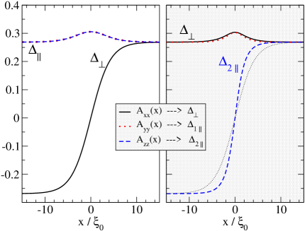
Figure 1: The order parameter profile across the domain wall ($\Delta$ is in units of $2\pi k_{B}T_{c}$, $\xi_{0}=\hbar v_{f}/2\pi k_{B}T_{c}$). Left panel: change in $\Delta_{\perp}$ across the wall, $A_{xx}(-x)=-A_{xx}(x)$. In this case $\Delta_{1\,\parallel}=\Delta_{2\,\parallel}=\Delta_{\parallel}$. Right panel: $\Delta_{2\,\parallel}$ changes sign, $A_{zz}(-x)=-A_{zz}(x)$, and $\Delta_{1\,\parallel}$ is slightly different from $\Delta_{\perp}$. For comparison the thin dotted line is $\Delta_{\perp}$ from the left panel. The parallel domain wall is thinner than the “perpendicular” domain wall by a factor of about $1.8$.

The self-consistent solutions for the two order parameter configurations are shown in Fig. 1. We see when $\Delta_{\parallel}$ changes sign (right panel) the domain wall is approximately twice as narrow as than the domain wall in which $\Delta_{\perp}$ changes sign. This means that the deformation of the superfluid order parameter is weaker for the case of the “parallel” domain wall. The difference in the order parameter structures between these two domain walls is qualitatively explained by difference in the number of trajectories that are pairbreaking. In the “perpendicular” configuration the pairbreaking trajectories are predominantly perpendicular to the domain wall. In the case of the “parallel” domain wall trajectories that are nearly parallel to domain wall are most pairbreaking. However, these trajectories only weakly connect the two sides of the domain wall. As a result the profile of the order parameter is narrower than that of the perpendicular domain wall.

We explore this feature further by computing the free energy for each given order parameter profile. The free energy is calculated by introducing the auxiliary propagator $\widehat{g}_{\lambda}$ that satisfies the transport equation,

$$\left[i\varepsilon_{m}\widehat{\tau}_{3}-\lambda\,\widehat{\Delta},\widehat{g}_{\lambda}\right]+i{\bf v}_{f}\cdot\mbox{\boldmath$\nabla$}\widehat{g}_{\lambda}=0\,,$$ (7)

with $0\leq\lambda\leq 1$. The free energy in the weak coupling limit can be expressed as an integral over the variable coupling constant, $\lambda$,[6]

$${\mbox{\footnotesize$\Delta$}}\Omega=\frac{\mbox{\small 1}}{\mbox{\small 2}}\int_{0}^{1}\,d\lambda\,\mbox{Sp}^{\prime}\left\{\widehat{\Delta}\,\left(\widehat{g}_{\lambda}-\frac{\mbox{\small 1}}{\mbox{\small 2}}\widehat{g}\right)\right\}\equiv\int d^{3}R\;{\mbox{\footnotesize$\Delta$}}F({\bf R})\,.$$ (8)

We define the free energy density, ${\mbox{\footnotesize$\Delta$}}F({\bf R})$, from the definition of the trace, $\mbox{Sp}^{\prime}$, which stands for summation and integration over all indices and variables, e.g.

$$\mbox{Sp}^{\prime}\left\{\widehat{\Delta}\,\widehat{g}\right\}\equiv\int d^{3}R\left\{T\sum_{\varepsilon_{m}}N_{f}\,\int\frac{d\Omega_{\hat{\bf p}}}{4\pi}\mbox{Tr}_{4}\big{(}\widehat{\Delta}(\hat{\bf p},{\bf R})\widehat{g}(\hat{\bf p},{\bf R};\varepsilon_{m})\big{)}\right\}\,.$$

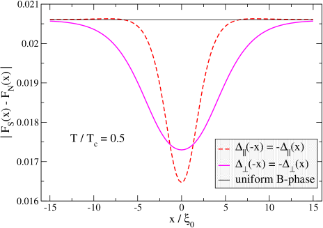
Figure 2: Reduction of the condensation energy near a domain wall [in units $N_{f}(2\pi k_{B}T_{c})^{2}$]. The magnitude of the free energy density for the “parallel” configuration is suppressed more around $x=0$ due to the larger gradient energy terms, but the integrated suppression is less than that for the “perpendicular” configuration.

The free energy densities for the two domain walls are shown in Fig. 2. The change in $\Delta_{2\,\parallel}$ takes place over a shorter distance than that of $\Delta_{\perp}$. Thus, the former configuration has larger gradient energy. Nevertheless, this is compensated by the spatial extent of “perpendicular” domain wall with the result that the net energy cost of the “parallel” domain wall is less than that of the ”perpendicular” domain wall. This result has implications for the structure of the order parameter and the stability of new phases of superfluid ³He in confined geometry.

We demonstrate this point by the following argument. Fig. 3 shows a slab of ³He-B and two types of quasiparticle trajectories. Trajectory $1$ undergoes a reflection from a boundary, while trajectory $2$ is a straight trajectory in the region of interest. In case (a) shown in Fig. 3 the order parameter component $A_{zz}$ has the same sign to the left and right of the vertical line. Thus, quasiparticles moving on trajectory $1$ propagate in a changing order parameter field, $\Delta_{z}\to-\Delta_{z}$, which is equivalent to the “perpendicular” domain wall. However, quasiparticles moving along trajectory $2$ do not experience a change in the sign of the order parameter.

Case (b) shown in Fig. 3 is quite different. In this case we assume a domain wall in which $A_{zz}$ changes sign on the two sides. Now quasiparticles moving on trajectory $1$ do not experience a sign change because the change in the momentum, $\hat{p}_{z}\to\,-\hat{p}_{z}$, is compensated by the sign change in $A_{zz}$. Thus, there is no contribution to the order parameter deformation from this trajectory. However, this reduction in surface pairbreaking occurs at the cost of pairbreaking introduced trajectories of the second type. Quasiparticles moving on trajectory $2$ propagate through an order parameter field with a sign change. But since these type of trajectories lead to a domain wall of the “parallel” type, the domain wall structure may be favorable to the uniform solution in the thin film shown in case (a).

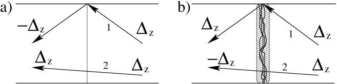
Figure 3: Pairbreaking trajectories with and without a domain wall in the ³He-B film. a) no domain wall, b) $A_{zz}(x)$ changes sign from left to right.

This observation about the possible stability of domain wall structures depends on the thickness of the slab or film since for very thick films it is clearly unfavorable to have domain walls in the plane of the film. However, for thinner films or slabs inhomogeneous structures related to parallel domains are possible. A full quasiclassical calculation of the structure and free energy for thin films of superfluid ³He confirms this observation based on the domain wall calculations. We have found that associated with the domain wall structures new order parameter components develop, and that there are periodic structures formed from domain walls along the plane of the film that are energetically favorable compared to an order parameter that is translationally invariant in the plane of the film. We find a range of film thickness, $10\xi_{0}-12\xi_{0}$, for which these inhomogeneous states are favored. The details of this calculation will be published elsewhere.

We thank Tomas Löfwander and Erhai Zhao for useful comments on this work.

References

- [1] V. Ambegaokar, P. deGennes, and D. Rainer, Phys. Rev. A9, 2676 (1975).
- [2] W.Zhang, J.Kurkijärvi, and E.V.Thuneberg, Phys. Rev. B 36, 1987 (1987).
- [3] E. V. Thuneberg, M. Fogelström, and J. Kurkijärvi, Physica B 178, 176 (1992).
- [4] Y. Nagato, M. Yamamoto, and K. Nagai, J. Low Temp. Phys. 110, 1135 (1998).
- [5] J. W. Serene and D. Rainer, Phys. Rep. 101, 221 (1983).
- [6] A. Vorontsov and J. A. Sauls, Phys. Rev. B 68, 064508 (2003).