Vortices and Ring Solitons in Bose-Einstein Condensates

Abstract

The form and stability properties of axisymmetric and spherically symmetric stationary states in two and three dimensions, respectively, are elucidated for Bose-Einstein condensates. These states include the ground state, central vortices, and radial excitations of both. The latter are called ring solitons in two dimensions and spherical shells in three. The nonlinear Schrodinger equation is taken as the fundamental model; both extended and harmonically trapped condensates are considered. It is found that instability times of ring solitons can be long compared to experimental time scales, making them effectively stable over the lifetime of an experiment.

I Introduction

One of the primary motivations in the original derivation of the Gross-Pitaevskii equation was to describe vortices in superfluids pitaevskii1961 ; gross1961 ; fetter1972 . The quantization of vorticity is a central difference between classical fluids and superfluids donnelly1991 . The Gross-Pitaevskii equation has proven to be an excellent model for weakly interacting, dilute atomic anderson1995 ; davis1995 ; bradleyCC1995 ; bradleyCC1997 ; dalfovo1999 ; leggett2001 and molecular greiner2003 ; jochim2003b ; zwierlein2003 Bose-Einstein condensates (BEC’s), which are generally superfluid. In the context of optics the Gross-Pitaevskii equation is known as the nonlinear Schrödinger equation (NLSE) agrawal1995 . Vortices matthews1999 ; madison2000 , as well as their one-dimensional analog, solitons burger1999 ; denschlag2000 , have been observed in BEC’s in numerous experiments. The NLSE describes these observations well ruprecht1995 ; fetter2001 ; feder1999 ; williams1999 .

However, there are in fact much richer vortex and soliton structures yet to be observed. One such structure is the ring soliton theocharis2003 ; kivshar1994 ; dreischuh1996 ; frantzeskakis2000 ; nistazakis2001 ; neshev1997 ; dreischuh2002 , a soliton extended into two dimensions which loops back on itself to form a ring, i.e., a radial node. This appears as an axisymmetric radial node of the condensate; set at the right distance from the origin, it becomes a stationary state. In the optics context, the ring soliton is well known to be unstable to the snake instability, whereby it decays into vortex-anti-vortex pairs. In this article, we not only describe vortices and radially excited states of BEC’s with high precision, but we also show that in a harmonic trap the decay time can be long compared to the classical oscillation period of the trap and even the lifetime of the condensate itself optics .

We consider three cases for the external, or trapping potential $V(\vec{r})$. First, $V(\vec{r})=0$ corresponds to an infinitely extended condensate and leads to solutions of beautiful mathematical form. Second, $V(\vec{r})=V(r)=0$ for $r\leq R$ and $V(r)=\infty$ for $r>R$, corresponds to a disk in two dimensions and a sphere in three, i.e., an infinite well. This introduces confinement into the problem, connects heuristically with the first case and general knowledge of solutions to Schrödinger equations, and serves as a bridge to the experimental case of a harmonic trap. Third, $V(\vec{r})=\frac{1}{2}M[\omega^{2}(x^{2}+y^{2})+\omega_{z}^{2}z^{2}]$, with $\omega\ll\omega_{z}$, where $M$ is the atomic mass and $\omega,\omega_{z}$ are the classical oscillation frequencies, corresponds to a highly oblate harmonic trap, which is most relevant to present experiments.

This work follows in the spirit of a previous set of investigations of the one-dimensional NLSE, for both repulsive and attractive nonlinearity carr2000a ; carr2000b . In that work it was possible to obtain all stationary solutions in closed analytic form. In the present cases of two and three dimensions, we are unaware of an exhaustive class of closed form solutions but instead use a combination of analytical and numerical techniques to elicit the stationary and stability properties of similar solutions. Here, we treat the case of repulsive atomic interactions; as in our previous work on one dimension, the attractive case has been treated separately carr2004k , due to the very different character of the solutions.

Equations similar to the NLSE are often used as models for classical and quantum systems. Thus a tremendous amount of theoretical work has been done on vortices, to which the reader is referred to Fetter and Svidzinsky on BEC’s fetter2001 , Donnelly on Helium II donnelly1991 , and Saffman on classical vortices saffman1992 as good starting points for investigations of the literature. As NLSE-type equations apply in many physical contexts, our results are widely applicable beyond the BEC.

The article is outlined as follows. The derivation of the fundamental differential equations is presented in Sec. II. In Sec. III the ground state and vortices in two dimensions are presented. In Sec. IV the stationary radial excitations of these solutions are illustrated. In Sec. V the ground state and its radial excitations in three dimensions are treated. In Sec. VI the stability properties of solution types containing ring solitons are discussed. Finally, in Sec. VII, we discuss the results and conclude.

II Fundamental Equation

The fundamental differential equation is derived as follows. The NLSE, which models the mean field of a BEC pitaevskii1961 ; gross1961 ; dalfovo1999 , is written as

$$\left[-\frac{\hbar^{2}}{2M}\nabla^{2}+g\,|\psi|^{2}+V(\vec{r})\right]\psi=i\hbar\frac{\partial}{\partial t}\psi\,,$$ (1)

where $V(\vec{r})$ is an external potential, $g\equiv 4\pi\hbar^{2}a_{s}/M$, $a_{s}$ is the $s$-wave scattering length for binary interaction between atoms with $a_{s}>0$, since this is the repulsive case, and $M$ is the atomic mass. The condensate order parameter $\psi=\psi(\vec{r},t)\equiv\sqrt{n(\vec{r},t)}\exp[iS(\vec{r},t)]$, where $n(\vec{r},t)$ is the local atomic number density and $\vec{v}(\vec{r},t)=(\hbar/M)\vec{\nabla}S(\vec{r},t)$ is the local superfluid velocity. Note that, in two dimensions, the coupling constant $g$ is renormalized by a transverse length petrov2000 ; olshanii1998 ; petrov2000b ; carr2000e .

We assume cylindrical or spherical symmetry of both the external potential and the order parameter in two or three dimensions, respectively. This has the effect of reducing Eq. (1) to one non-trivial spatial variable. Specifically, wavefunctions of the form

$$\psi(\vec{r})=f_{m}(r)\exp(im\phi)\exp(-i\mu t/\hbar)\exp(i\theta_{0})$$ (2)

are treated, where $m$ is the winding number, $\mu$ is the eigenvalue, also called the chemical potential, $\phi$ is the azimuthal coordinate, $r$ is the radial coordinate in two or three dimensions, and $\theta_{0}$ is a constant phase which may be taken to be zero without loss of generality.

Assuming an axisymmetric stationary state in two dimensions of the form given in Eq. (2), Eq. (1) becomes

$$-\frac{\hbar^{2}}{2M}\left(\frac{\partial^{2}}{\partial r^{2}}+\frac{1}{r}\frac{\partial}{\partial r}-\frac{m^{2}}{r^{2}}\right)f_{m}$$

$$+gf_{m}^{3}+V(r)f_{m}-\mu f_{m}=0\,.$$ (3)

Assuming spherical symmetry in three dimensions, one finds a similar equation,

$$-\frac{\hbar^{2}}{2M}\left(\frac{\partial^{2}}{\partial r^{2}}+\frac{2}{r}\frac{\partial}{\partial r}\right)f_{0}+gf_{0}^{3}+V(r)f_{0}-\mu f_{0}=0\,.$$ (4)

In Eq. (4) it is assumed that $m=0$, in keeping with the spherical symmetry. This is an important special case, as it includes the ground state. In the remainder of this work, $m$ will be taken as non-negative since $f_{-|m|}=f_{|m|}$.

The physically relevant solutions of Eqs. (3) and (4) include the ground state, vortices, ring solitons, and spherical shells, as we will show in the following three sections. A variety of solution methods are used to treat the wavefunction in different regions of $r$, as discussed in Appendix A. Different rescalings of Eqs. (3)-(4) are appropriate for the three potentials we consider: constant, infinite well, and oblate harmonic. These are treated briefly in the following subsections.

II.1 Constant Potential

A constant potential has no direct experimental realization. However, it does have mathematical properties which are helpful in understanding the confined case, not to mention beautiful in themselves. For instance, the vortex solution manifests as a boundary between divergent and non-divergent solutions, as shall be explained.

The potential $V(r)=V_{0}$ can be taken to be zero without loss of generality. Then the variables can be rescaled as

$$\eta_{m} \equiv \sqrt{\frac{g}{\mu}}f_{m}\,,$$ (5)

$$\chi \equiv \frac{\sqrt{2M\mu}\,r}{\hbar}\,.$$ (6)

Note that the radial coordinate is scaled to the length associated with the chemical potential. Then Eq. (3) becomes

$$\eta_{m}^{\prime\prime}+\frac{1}{\chi}\eta_{m}^{\prime}-\frac{m^{2}}{\chi^{2}}\eta_{m}-\eta_{m}^{3}+\eta_{m}=0\,,$$ (7)

and Eq. (4) becomes

$$\eta_{0}^{\prime\prime}+\frac{2}{\chi}\eta_{0}^{\prime}-\eta_{0}^{3}+\eta_{0}=0\,,$$ (8)

where $\mu$ has been assumed to be positive, since this is the physically meaningful case for repulsive atomic interactions. Note that, in these units, the length scale of a vortex core is on the order of unity.

II.2 Infinite Potential Well in Two and Three Dimensions

Let us first consider the two dimensional infinite well. A confined condensate may be obtained by placing an infinite potential wall at fixed $r=\sqrt{x^{2}+y^{2}}$, at any node of the wavefunction $\psi(r,\phi)$. This treats either a condensate tightly confined in $z$ or a cylinder of infinite $z$ extent. In either case, one derives a 2D NLSE from the 3D one by projecting the $z$ degree of freedom onto the ground state and integrating over it. This leads to a straightforward renormalization of the coefficient of the nonlinear, cubic term. Extremely high potential wells in the $x$-$y$ plane have been created in BEC experiments via higher order Gauss-Laguerre modes of optical traps bongs2001 .

For the purposes of our numerical algorithm outlined in Appendix A, it is convenient to keep the same scalings as Eqs. (5)-(6). Then the normalization has to be treated with some care. The normalization of $\psi$ in two dimensions for a BEC of $N$ atoms in an infinite cylindrical well of radius $R$ is given by

$$\int_{0}^{2\pi}d\phi\int_{0}^{R}dr\,r|\psi(r,\phi;t)|^{2}=N\,.$$ (9)

After the change of units given by Eqs. (5) and (6) the normalization becomes

$$\int_{0}^{\chi_{R}}d\chi\,\chi[\eta_{m}(\chi)]^{2}=2\mathcal{N}\,,$$ (10)

where

$$\mathcal{N}\equiv\frac{M}{2\pi\hbar^{2}}gN\,,$$ (11)

$$\chi_{R}\equiv\sqrt{\frac{2M\mu}{\hbar^{2}}}R$$ (12)

are the effective nonlinearity and cylinder radius.

The three-dimensional infinite well is treated similarly, with the normalization being $\mathcal{N}$, rather than $2\mathcal{N}$, due to the extra angular integration.

The details of the algorithm for calculation of quantized modes in two and three dimensions is discussed in Appendix A.4.

II.3 Oblate Harmonic Trap

For the harmonic potential we shall focus on the case of a highly oblate trap, which is the experimentally relevant one to obtain axial symmetry in two effective dimensions ketterle1999 . Then, again projecting onto the ground state in $z$, the rescaled nonlinearity $\mathcal{N}$ has a simple interpretation:

$$\mathcal{N}=2a_{s}N\sqrt{M\omega_{z}/2\pi\hbar}\,,$$ (13)

where $\omega_{z}$ is the angular frequency of the trap in the $z$ direction. The trap is isotropic in the remaining two directions, $\omega\equiv\omega_{x}=\omega_{y}$. All energies can then be scaled to $\hbar\omega$, lengths to $\ell\equiv\sqrt{\hbar/M\omega}$, etc., as follows:

$$-\frac{1}{2}\left(\tilde{f}_{m}^{\prime\prime}+\frac{1}{\tilde{r}}\tilde{f}_{m}^{\prime}-\frac{m^{2}}{\tilde{r}^{2}}\tilde{f}_{m}\right)+\tilde{f}_{m}^{3}+\frac{1}{2}\tilde{r}^{2}\tilde{f}_{m}-\tilde{\mu}\tilde{f}_{m}=0\,,$$ (14)

where the tildes refer to harmonic oscillator scalings. Explicitly, $\tilde{r}\equiv r/\ell$, $\tilde{f}_{m}\equiv\ell f_{m}$, $\tilde{\mu}\equiv\mu/\hbar\omega$, and the normalization is

$$\int d\tilde{r}\,\tilde{r}\,|\tilde{f}_{m}|^{2}=\mathcal{N}\,.$$ (15)

The main difference between Eqs. (14) and Eq. (7) is that an extra parameter must be set in the numerical algorithm of Appendix A, i.e., the rescaled chemical potential. Then the normalization is determined from Eq. (15).

III Ground State and Vortices

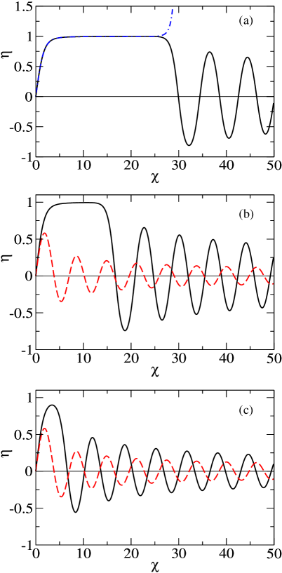
Figure 1: (color online) Approaching the vortex solution. Shown is the dependence of the wavefunction on the precision in the critical determining coefficient $a_{0}^{(m=1)}$ for a quantum vortex stationary state of the nonlinear Schrödinger equation in two dimensions. (a) The vortex solution forms a boundary between convergent ($a_{0}=a_{0}^{(1)}(1-10^{-16})$, solid black curve) and divergent ($a_{0}=a_{0}^{(1)}(1+10^{-16})$, dot-dashed blue curve) solutions. As the precision is reduced, the first node moves towards the origin and the solution approaches the Bessel function: (b) 8 digits of precision; (c) 2 digits of precision. In (b) and (c) the regular Bessel function solution to the linear Schrödinger equation is shown for comparison abramowitz1964 (dashed red curve). Note that all axes are dimensionless.

In order to solve Eqs. (3) and (4), we use a numerical shooting method, as discussed in App. A.3. Two initial conditions are required, as the NLSE is second order. These are provided by a Taylor expansion around $\chi=0$, as described in Sec. A.1. By this method a single parameter is sufficient to determine the solution. This parameter, $a_{0}$, is the lowest non-zero coefficient in the Taylor series. High precision is required, as discussed in the appendix, with the number of digits of precision determining where the numerical method either converges or diverges.

For the first potential we consider, $V(\chi)=0$, the ground state, which is obtained for $m=0$, lies precisely on the border between convergence and divergence of the algorithm. The value of $a_{0}$ which is exactly on this border we term $a_{0}^{(0)}$. The wavefunction $\eta_{0}(\chi)$ is constant and, according to our scalings, is simply $\pm\sqrt{\mu/g}=\pm 1$. Then $a_{0}^{(0)}=\pm 1$ and the precision is infinite. Values of $|a_{0}|$ larger than 1 lead to a divergent solution, while values of $|a_{0}|$ less than 1 lead to a convergent one. In the latter case the wavefunction oscillates an infinite number of times and approaches zero, as will be discussed in Sec. IV. Thus, in general, $|\eta_{0}|$ can approach only three asymptotic values: 0, 1, and $\infty$.

For the case of non-zero winding number, one finds a central vortex. As in the case of the ground state, $\lim_{\chi\rightarrow\infty}|\eta_{m}|^{2}\equiv\bar{n}=\mu/g$ is the asymptotic density of the vortex state. In this region the spatial derivatives yield zero and $\eta_{m}(\chi)\rightarrow\pm 1$ as $\chi\rightarrow\infty$. The vortex again lies on the border between divergence and convergence of our algorithm, given by a single parameter $a_{0}^{(m)}$ which determines the whole Taylor series. In Appendix A the precision issues are discussed in detail. In Fig. 1 is illustrated the algorithmic approach to the vortex solution for zero external potential. The effect of the number of digits of precision is shown in detail, and further explained in Appendix A, where the best values of $a_{0}^{(m)}$ for winding numbers $m=1$ to $m=5$ are given.

For the second potential, an infinite well in two dimensions, the properly normalized ground state and vortex states are produced by the simple prescription give in Appendix A.4. An example is shown for $m=1$ in Fig. 2(a). The ground state for three dimensions can be found by a similar method, and is shown for $m=0$ in Fig. 6(a).

For the third potential, a strongly oblate harmonic trap, the form and stability of both the ground state and vortex solutions in a harmonic trap have already been thoroughly studied elsewhere ruprecht1995 ; dodd1996a ; pu1999 . Our algorithm reproduces all the relevant results of these authors from the non-interacting to the Thomas-Fermi regime, as we explicitly verified in detail in the case of Ref. pu1999 .

IV Ring Solitons

Ring solitons can be placed concentrically to form a stationary state. In an extended system a denumerably infinite number are required, as already indicated in Fig. 1 and discussed in further detail in Sec. IV.3 below. For an infinite well in two dimensions, radially quantized modes are distinguished by the number of concentric ring solitons, as discussed in Sec. IV.1 and illustrated in Fig. 2. Note that, for attractive nonlinearity, the number of rings can vary from one to infinity, even for an infinitely extended condensate, as discussed in Ref. carr2004k .

IV.1 Quantized Modes in the Cylindrical Infinite Well

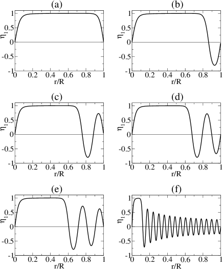
Figure 2: Ring solitons in an infinite well. Shown is the form of the wavefunction $\eta_{1}$ for (a) the ground state, (b)-(e) the first four axisymmetric excited states, and (f) a highly excited state, all as a function of the radial coordinate $r$ scaled to the cylinder size $R$. Cylindrical box boundary conditions in cylindrical polar coordinates are assumed. The central vortex has winding number $m=1$. The quantized modes (b)-(f) correspond to increasing numbers of concentric ring solitons. Here, the case of strong nonlinearity is illustrated, with $2\mathcal{N}=402$. Note that all axes are dimensionless.

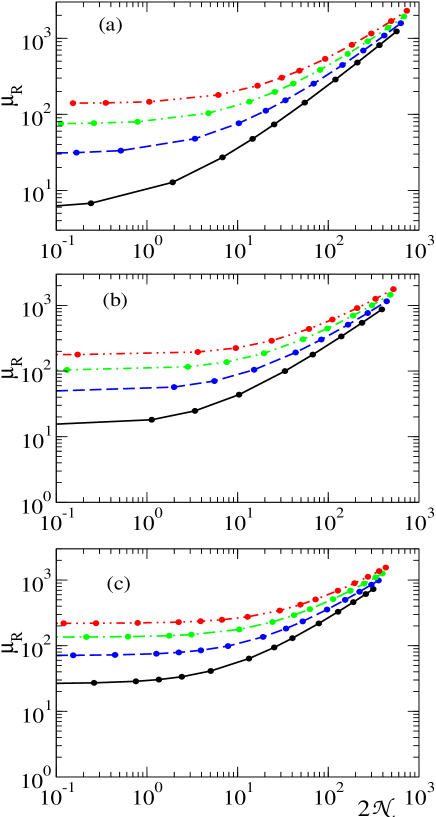
Figure 3: (color online) Ring solitons in an infinite well. Shown are the eigenvalue spectra $\mu_{R}$ as a function of the normalization $2\mathcal{N}$. The winding numbers (a) $m=0$, (b) $m=1$, and (c) $m=2$ are illustrated for the ground state (solid black curve), and the first three excited states (blue dashed, green dot-dashed, and red double-dot-dashed curves). The circles show the actual data points. Note that all axes are dimensionless as indicated in the text, and on the same log-log scale.

In Fig. 2 are shown the wavefunctions for the ground state and first three excited states for a fixed strong nonlinearity $\mathcal{N}$ in the presence of a singly quantized central vortex, i.e., winding number $m=1$. The weaker the nonlinearity and the larger the number of nodes in the solution, the closer it resembles the regular Bessel function $J_{m}(\chi)$. In an appropriately scaled finite system, the relative weight of the kinetic term to the mean field term in the NLSE increases strongly with the number of nodes. We note the contrast with the distribution of nodes for the corresponding 1D NLSE carr2000a ; carr2000b , where the nodes are evenly spaced even in the extremely nonlinear limit. The value of the nonlinearity was chosen to be $2\mathcal{N}=402$. For transverse harmonic confinement of angular frequency $\omega_{z}=2\pi\times 100$ Hz and ⁸⁷Rb, which has a scattering length of $a_{s}=5.77$ nm, this corresponds to $N\simeq 10,000$ atoms. Note that, since $\eta$ is scaled to $g/\mu$, and $\mu$ depends on the number of nodes, the vertical scaling is different in each panel of Fig. 2.

The eigenvalue spectra for the ground state and the first two excited states are shown in Fig. 3, with $\mu$ scaled to the radius of the infinite well,

$$\mu_{R}\equiv\frac{2MR^{2}}{\hbar^{2}}\mu\,.$$ (16)

The winding numbers $m=0$, $m=1$, and $m=2$ are illustrated on a log-log scale. Clearly there are two regimes. For small $\mathcal{N}$, $\mu_{R}$ is independent of the norm. This must be the case near the linear-Schrödinger-equation regime, since $\mu_{R}$ must approach the eigenvalues of the regular Bessel function $J_{m}(\chi)$ which solves Eq. (7) with no cubic term. One finds $(\mu_{R})_{j}\rightarrow(\chi_{j}^{\mathrm{linear}})^{2}$, where $\chi_{j}^{\mathrm{linear}}$ is the known value of the $j^{\mathrm{th}}$ node of the Bessel function abramowitz1964 and $j$ also refers to the $j^{\mathrm{th}}$ quantized mode.

For large $\mathcal{N}$, the figure shows that $\mu_{R}\propto\mathcal{N}$. This dependence can be understood analytically in the case of the Thomas-Fermi-like profile dalfovo1999 for the lowest energy state with winding number $m=1$. Consider the scaling

$$\rho \equiv r/R\,$$ (17)

$$\kappa(\rho) \equiv \frac{1}{\sqrt{N}}f_{m}(r/R)\,.$$ (18)

Then Eq. (3) becomes

$$\frac{\partial^{2}\kappa}{\partial\rho^{2}}+\frac{1}{\rho}\frac{\partial\kappa}{\partial\rho}-\frac{m^{2}}{\rho^{2}}\kappa-4\pi R^{2}\mathcal{N}\kappa^{3}+\mu_{R}\kappa=0\,.$$ (19)

The Thomas-Fermi profile is obtained by dropping the derivatives:

$$\kappa_{\mathrm{TF}}(\rho)=\sqrt{\frac{\mu_{R}}{4\pi R^{2}\mathcal{N}}\left(1-\frac{\rho_{m}^{2}}{\rho^{2}}\right)}\,$$ (20)

where

$$\rho_{m}\equiv\frac{m}{\sqrt{\mu_{R}}}$$ (21)

is the core size and $\kappa_{\mathrm{TF}}$ is zero for $\rho\leq\rho_{m}$. The normalization condition is

$$2\pi R^{2}\int_{\rho_{m}}^{1}d\rho\,\rho\left[\kappa_{\mathrm{TF}}(\rho)\right]^{2}=1\,.$$ (22)

Then the chemical potential in units of the energy associated with the cylinder radius is

$$\mu_{R}=\frac{4\mathcal{N}}{1-\rho_{m}^{2}+\rho_{m}^{2}\ln(\rho_{m}^{2})}\,.$$ (23)

The limit $\rho_{m}\ll 1$ is consistent with the Thomas-Fermi-like profile, which neglects the radial kinetic energy. In this limit, one finds

$$\mu_{R}\simeq 4\mathcal{N}\left[1+\rho_{m}^{2}-\rho_{m}^{2}\ln\left(\rho_{m}^{2}\right)\right]\,.$$ (24)

For $\rho_{m}^{2}\leq 0.03$, as is the case in the right hand side of Fig. 3(a)-(c) where $\mu_{r}\simeq 10^{3}$, the dependence on $\rho_{m}^{2}$ is a less than 1% perturbation.

IV.2 Quantized Modes in the Strongly Oblate Harmonic Trap

In figure 4 is shown the wavefunction for fixed strong nonlinearity for the ground state and first three excited states. As in Sec. IV.1, adding nodes to the wavefunction drives the system towards the linear regime, where the solution is Bessel-function-like. In Fig. 5 are shown the spectra for the ground state and first three excited states, for a winding number of $m=0,1,2$. Note that the chemical potential is rescaled to the harmonic oscillator energy. As in Sec. IV.1, there are two regimes. For large nonlinearity a Thomas-Fermi approximation can be applied to obtain the asymptotic dependence of the chemical potential on the nonlinearity, similar to the procedure of Sec. IV.1.

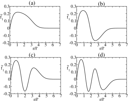
Figure 4: Ring solitons in a harmonic trap. Shown is the form of the wavefunction $\tilde{f}_{1}$ for (a) the ground state and (b)-(d) the first three axisymmetric excited states, all as a function of the radial coordinate $\tilde{r}$. The harmonic trap is strongly oblate, so that it is effectively two-dimensional. The central vortex has winding number $m=1$. The quantized modes (b)-(d) correspond to increasing numbers of concentric ring solitons. Here, the case of strong nonlinearity is illustrated for (a), with $\mathcal{N}=100$; for three rings, i.e., (d), the solution already appears nearly linear. Note that the tildes signify that all axes are in harmonic oscillator units.

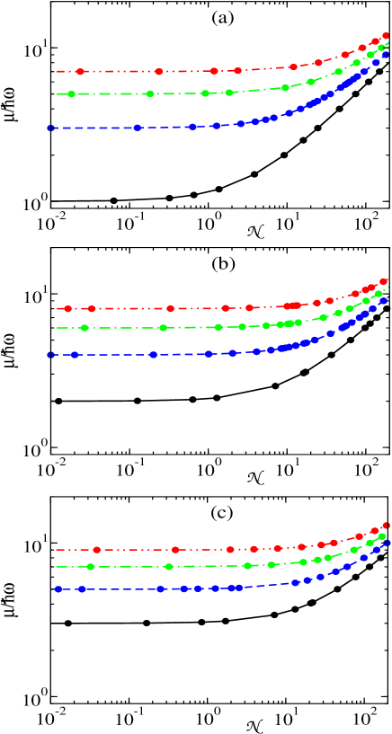
Figure 5: Ring solitons in a harmonic trap. Shown are the eigenvalue spectra $\mu$ as a function of the normalization $\mathcal{N}$, all in harmonic oscillator units. The ground state (solid black curve) and the first three isotropic excited states (blue dashed, green dot-dashed, and red double-dot-dashed curves) are illustrated for a winding number of (a) $m=0$, (b) $m=1$ and (c) $m=2$. The circles show the actual data points. Note that all axes are dimensionless and on a log-log scale.

IV.3 Asymptotic Behavior for Zero External Potential

For $\chi\rightarrow\infty$ and $|a_{0}|<|a_{0}^{(m)}|$ the wavefunction approaches zero in an infinitely extended system. Thus one expects that the nonlinear term $\eta^{3}$ in Eq. (7) is negligible in comparison to the other terms, and the differential equation returns to the usual defining equation for the Bessel functions. The asymptotic form of the regular Bessel function $J_{m}(\chi)$ is abramowitz1964

$$J_{m}(\chi)=\sqrt{\frac{2}{\pi\chi}}\cos\left[\chi-\frac{m\pi}{2}-\frac{\pi}{4}\right]\,,$$ (25)

to leading order in the amplitude and the phase. However, one cannot neglect the effect of the cubic term on the phase shift, as may be seen by the following considerations.

The asymptotic form of the Bessel function can be derived via the semiclassical WKB approximation brack1997 . The phase shift of $\pi/4$ can be derived by analytical continuation or other means landau1977 . The semiclassical requirement that the de Broglie wavelength be small compared to the length scale of the change in potential is not quite satisfied near the origin. The rescaling $y=y_{0}\ln(\chi)$ suffices to map the problem onto the usual semiclassical one. One can avoid the rescaling by the substitution $m^{2}\rightarrow m^{2}-\frac{1}{4}$. Then the term $m\pi/2$ in the phase shift follows directly langer1937 ; berry1972 . We use this simpler method in order to derive the phase shift in the nonlinear problem.

The semiclassical momentum is

$$p(\chi)\equiv\sqrt{1-V_{\mathrm{eff}}(\chi)}\,,$$ (26)

where the effective potential is

$$V_{\mathrm{eff}}(\chi)=\frac{m^{2}}{\chi^{2}}+[\eta_{m}(\chi)]^{2}\,.$$ (27)

Taking the nonlinear term as perturbative, to lowest order Eq. (27) becomes

$$V_{\mathrm{eff}}(\chi) \simeq \frac{m^{2}}{\chi^{2}}+\frac{B^{2}}{\chi}\cos^{2}\left(\theta_{m}\right)\,,$$ (28)

$$\theta_{m} \equiv \chi-\frac{m\pi}{2}-\frac{\pi}{4}\,,$$ (29)

where $B$ is a constant coefficient of the amplitude of the wavefunction. In the linear case, it is conventionally taken as $B=\sqrt{2/\pi}$. Expanding Eq. (26) for large $\chi$, one finds

$$p(\chi)\simeq 1-\frac{B^{2}\cos^{2}\theta_{m}}{2\chi}-\frac{m^{2}+\frac{1}{8}B^{4}\cos^{4}\theta_{m}}{2\chi^{2}}\,.$$ (30)

The semiclassical form of the wavefunction is brack1997 ; landau1977

$$\eta_{m}\simeq\frac{B}{\sqrt{\chi}}\cos\left(S-\frac{\pi}{4}\right)$$ (31)

to leading order, where

$$S\equiv\int_{0}^{\chi}d\chi^{\prime}\,p(\chi^{\prime})\,$$ (32)

is the semiclassical action. Upon substitution of Eq. (30) one finds the form of the wavefunction to leading order in the amplitude and the phase,

$$\eta_{m}\simeq\frac{B}{\sqrt{\chi}}\cos\left[\chi-\frac{B^{2}}{4}\ln(\chi)\right.$$

$$\left.-\frac{m\pi}{2}-\frac{\pi}{4}+\delta(a_{0},m)\right]\,,$$ (33)

where $\delta$ is a phase shift which depends on the determining coefficient $a_{0}$ and the winding number $m$. This coefficient cannot be analytically determined by Eq. (32) since the large $\chi$ form of the wavefunction was used, while the phase shift is due to its behavior in the small $\chi$ region. The amplitude coefficient $B$ is a free parameter, the square of which is related to the mean number density.

The form of Eq. (33) resembles that of the Coulomb function abramowitz1964 , in that it has a $\ln(\chi)$ dependence in the phase. This is due to the $1/\chi$ term in the effective potential in Eq. (28). It is in this sense that the nonlinear term in Eq. (7) cannot be neglected, even as $\eta\rightarrow 0$.

V Spherical Shells

Spherical shells are the three-dimensional analog of ring solitons. Quantized modes in the confined case involve successive numbers of nested nodal spherical shells. In this section, we will treat the two cases of zero potential and an infinite spherical well. A power series solution of Eq. (8) may be developed by substitution of Eq. (46). This leads to a solution similar to that of Sec. A.1. All coefficients in the power series are given as polynomials in the determining coefficient $a_{0}$, which is the value of the wavefunction at the origin. The special solution $\eta_{0}(\chi)=a_{0}=\pm 1$ is the ground state in an extended system. Thus $a_{0}^{(0)}=\pm 1$. Positive values of $a_{0}$ which are larger than unity lead to a divergent solution. Those less than unity lead to a convergent solution which approaches zero as $\chi\rightarrow\infty$.

V.1 Quantized Modes in the Spherical Infinite Well

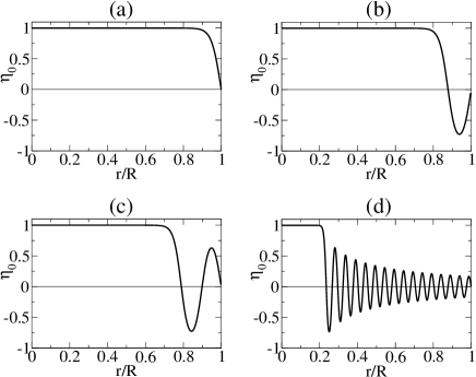
Figure 6: Spherical shell solutions. Shown is the form of the wavefunction for (a) the ground state, (b)-(c) the first two excited isotropic states, and (d) a highly excited isotropic state. The boundary conditions are an infinite spherical well in three dimensions. The winding number is zero. The case of strong nonlinearity is illustrated, with $\mathcal{N}=251$. Note that all axes are dimensionless.

Solutions can be quantized in the three-dimensional spherical well in the same way as the two-dimensional case. The solution methods are identical to those of Sec. IV.1. In Fig. 6 are shown the ground state, the first and second excited states, and a highly excited state. A fixed nonlinearity of $\mathcal{N}=251$ was chosen. In Fig. 7 is shown the eigenvalue spectra on a log-log scale. As in the two-dimensional case of Fig. 3, there are two regimes. For small $\mathcal{N}$, the eigenvalues are independent of the nonlinearity, $(\mu_{R})_{j}\rightarrow(\chi_{j}^{\mathrm{linear}})^{2}$. The constant $\chi_{j}^{\mathrm{linear}}$ is the distance to the $j$th nodes of the spherical Bessel function $j_{0}(\chi)$ which solves Eq. (8) with no cubic term abramowitz1964 . For large $\mathcal{N}$, one again finds a linear dependence. A simple estimate based on the Thomas-Fermi profile for $m=0$, which is just $f_{0}(r)=\mu/g$ for $r\leq R$ and zero otherwise, gives the chemical potential of the ground state as $\mu_{R}=\mathcal{N}/3$.

V.2 Asymptotic Behavior

As $r\rightarrow\infty$ the spherical shell wavefunction approaches zero in an infinitely extended system. Just as in Sec. IV.3, one can use the WKB semiclassical approximation method to determine the asymptotic form of the wavefunction. The solution to Eq. (8) without the cubic term is the spherical Bessel function abramowitz1964

$$j_{0}(\chi)=\frac{\sin\chi}{\chi}\,,$$ (34)

where we have assumed the wavefunction to be finite at the origin. One can take the nonlinear term as perturbative since, for sufficiently large $\chi$, the linear form of the wavefunction must dominate. Then the effective potential in the WKB formalism is

$$V_{\mathrm{eff}}(\chi)\simeq B^{2}\frac{\sin^{2}\chi}{\chi^{2}}\,,$$ (35)

where $B$ is the amplitude of the wavefunction. From Eqs. (26) and (32), the WKB action is

$$S\simeq\chi-\frac{B^{2}}{4}\frac{1}{\chi}+\delta^{\prime}(a_{0},m)$$ (36)

for large $\chi$, where the phase shift $\delta^{\prime}(a_{0},m)$ cannot be determined from the large $\chi$ behavior of the wavefunction. Then the asymptotic form of the wavefunction is

$$\eta_{0}(\chi)\rightarrow\frac{B}{\chi}\sin\left[\chi-\frac{B^{2}}{4\chi}+\delta^{\prime}(a_{0},m)\right]\,.$$ (37)

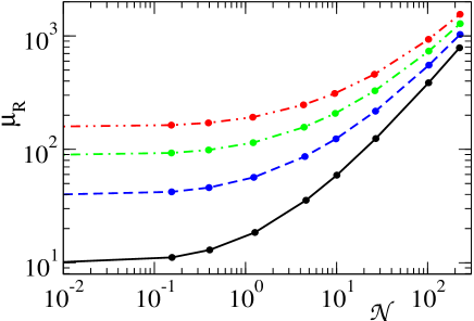
Figure 7: Spherical shell solutions. Shown are the eigenvalue spectra $\mu_{R}\equiv(2MR^{2}/\hbar^{2})\mu$ as a function of the normalization $\mathcal{N}$. The ground state (solid black curve) and the first three isotropic excited states (blue dashed, green dot-dashed, and red double-dot-dashed curves) are illustrated for a winding number of $m=0$. The circles show the actual data points. Note that all axes are dimensionless and on a log-log scale.

VI Stability Properties

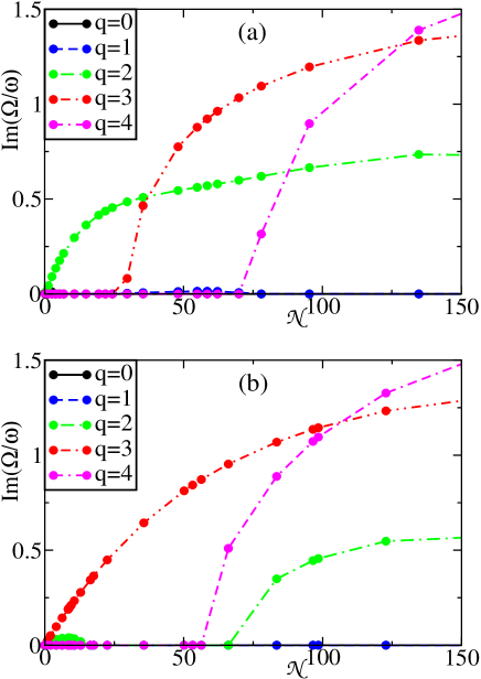
Figure 8: (color online) Stability Properties of Ring Solitons. Shown is the Boguliubov linear excitation frequency as a function of the nonlinearity $\mathcal{N}$, all in harmonic oscillator units. The index $q$ signifies the winding number of the Boguliubov mode. (a) A ring soliton with no central vortex; for $\mathcal{N}\lesssim 25$ the primary instability mode is $q=2$. (b) A ring soliton in the presence of a central vortex of winding number $m=1$; for $\mathcal{N}\lesssim 100$ the dominant instability is $q=3$. The solutions are always formally unstable, though instability times can be much longer than experimental timescales for small nonlinearities. The circles show the actual data points.

The stability properties of ring solitons in a strongly oblate harmonic trap are of particular importance, as such solutions may be realized in present experiments theocharis2003 . We perform linear stability analysis via the well-known Boguliubov de Gennes equations svidzinsky1998 ; fetter2001 :

$${\cal L}u_{j}-g\psi^{2}v_{j} = \hbar\Omega_{j}u_{j},$$ (38)

$${\cal L}v_{j}-g\left(\psi^{*}\right)^{2}u_{j} = -\hbar\Omega_{j}v_{j},$$ (39)

where

$${\cal L}\equiv-\frac{\hbar^{2}}{2M}\nabla^{2}+V(\vec{r})+2g|\psi|^{2}-\mu\,,$$ (40)

and $\Omega_{j}$ is the eigenvalue. In Eqs. (38)-(39) $u_{j}$ and $v_{j}$ are a complete set of coupled quasiparticle amplitudes that obey the normalization condition

$$\int d^{D}r\,\left(|u_{j}|^{2}-|v_{j}|^{2}\right)=1\,,$$ (41)

with $D$ the number of effective dimensions. These amplitudes represent excitations orthogonal to the condensate $\psi$. They have a straightforward quantum mechanical interpretation in terms of a canonical transformation of the second-quantized Hamiltonian for binary interactions via a contact potential of strength $g$ fetter2001 . Quasiparticles are superpositions of particles (creation operators) and holes (annihilation operators). Classically, they can be interpreted simply as linear perturbations to the condensate.

If the eigenvalue $\Omega_{j}$ is real, the solution $\psi$ is stable. If $\Omega_{j}$ has an imaginary part, then $\psi$ is unstable. There are significant subtleties in Boguliubov analysis; see the appendix of Ref. garay2001 for an excellent discussion. In the present effectively 2D potential with a condensate solution of the form given in Eq. (2), it is useful to redefine the Boguliubov amplitudes as suggested by Svidzinsky and Fetter svidzinsky1998 :

$$\pmatrix{u(\vec{r})\cr v(\vec{r})}=\frac{e^{iq\phi}}{\ell}\,\pmatrix{e^{im\phi}\,\tilde{u}_{q}(\tilde{r})\cr e^{-im\phi}\,\tilde{v}_{q}(\tilde{r})}\,,$$ (42)

where $\tilde{r}=\sqrt{x^{2}+y^{2}}/\ell$, $\ell$ is the harmonic oscillator length discussed in Sec. II.3, and we will neglect perturbations in the $z$ direction, due to the strongly oblate trap. Equation (42) represents a partial wave of angular momentum $q$ relative to the condensate. Then, in harmonic oscillator units (see Sec. II.3), Eqs. (38)-(39) become

$$\mathcal{L}_{+}\tilde{u}_{q}-|\tilde{f}_{m}|^{2}\tilde{v}_{q}=\frac{\Omega}{\omega}\tilde{u}_{q},$$ (43)

$$\mathcal{L}_{-}\tilde{v}_{q}-|\tilde{f}_{m}|^{2}\tilde{u}_{q}=-\frac{\Omega}{\omega}\tilde{v}_{q},$$ (44)

where

$$\mathcal{L}_{\pm} \equiv -\frac{1}{2}\left(\frac{\partial^{2}}{\partial\tilde{r}^{2}}+\frac{1}{\tilde{r}}\frac{\partial}{\partial\tilde{r}}-\frac{(q\pm m)^{2}}{\tilde{r}^{2}}-\tilde{r}^{2}\right)$$ (45)

$$+2|\tilde{f}_{m}|^{2}-\tilde{\mu}$$

The different centrifugal barriers inherent in $\mathcal{L}_{\pm}$ show that the two amplitudes behave differently near the origin, with $\tilde{u}_{q}\propto\tilde{r}^{|q+m|}$ and $\tilde{v}_{q}\propto\tilde{r}^{|q-m|}$ as $\tilde{r}\to 0$. Note that the nonlinear coefficient is absorbed into the normalization of $\tilde{f}_{m}$ – see Eq. (15).

The condensate wavefunction can be obtained via the shooting and Taylor expansion methods described in Appendix A. Then Eqs. (43)-(44) can be solved straightforwardly with standard numerical methods. We use a Laguerre discrete variable representation beck2000 ; mccurdy2003 , which is particularly efficient for this geometry, allowing us to go to hundreds of basis functions. The winding number $q$ of the Boguliubov modes was checked for $q=0$ to $q=6$ over the entire domain of our study.

The results are shown in Fig. 8. In panel (a), it is apparent that a single ring soliton placed on top of the ground state, i.e., with no central vortex, is always formally unstable to the quadrupole, or $q=2$ mode. The instability time is given by $T=-\omega/\mathrm{Im}(\Omega)$ in harmonic oscillator units. Typical trap frequencies range from $\omega=2\pi\times 10$ Hz to $2\pi\times 100$ Hz. Therefore, when $|\mathrm{Im}(\Omega)/\omega|\ll 1$, $T$ can be much longer than experimental time scales of 100 ms to 1 s. In this case, we say that the solution is experimentally stable. The instability time $T$ can even be longer than the lifetime of the condensate, the latter of which can range from 1 to 100 seconds. According to Fig. 8(a), this occurs for small nonlinearities. For larger nonlinearities, other modes, such as the octopole ($q=3$), also become unstable. In Fig. 8(b) is shown the case of single ring soliton in the presence of a singly quantized central vortex, i.e., $m=1$. The solution is again formally unstable, though first to octopole rather than quadropole perturbations. For small nonlinearities it is experimentally stable.

We did not quantitatively study solution stability for an infinite well. However, we expect that the boundary provides additional stability of ring solitons. To decay, ring solitons must break up into pairs of vortices via a transverse oscillation. To oscillate, the ring soliton has to move away from the barrier and inwards towards the origin. This requires shrinking the circumference of the ring, which costs energy, as a single ring feels an effective potential which pushes it outwards, as for example in an unbounded system. We expect that very long decay times follow. We make the conjecture that, in the infinitely extended system, the presence of an infinite number of rings, tightly pressed up against each other, has the same effect with regards to the inner ring as the boundary in the confined system.

VII Discussion and Conclusions

Soliton trains in one-dimensional BEC’s, which are similar to the nested ring solitons which form radial nodes, have been found to be archetypes of planar soliton motions encountered in three-dimensional BEC’s. These solutions to the one-dimensional NLSE are stationary states with islands of constant phase between equally spaced nodes. When appropriately perturbed, they give rise to soliton motion reinhardt1997 ; carr2000a . In fact, the stationary solutions can be considered to be dark solitons in the limiting case of zero soliton velocity, and the perturbation that produces propagating “gray” solitons is the imposition of a slight phase shift in the wavefunction across a node. These one-dimensional examples were found to have experimentally accessible analogs in three-dimensional BEC’s in which optically induced phase shifts across a plane of symmetry resulted in soliton motion burger1999 ; denschlag2000 ; feder2000 . Correspondingly, the two-dimensional ring solutions presented herein suggest the possibility of creating ring soliton motion by imposing a phase shift across the boundary of a disk. We will address this in subsequent work.

The existence of ring dark solitons has been predicted theoretically kivshar1994 ; dreischuh1996 ; frantzeskakis2000 ; nistazakis2001 and demonstrated experimentally neshev1997 ; dreischuh2002 in the context of nonlinear optics. It has been suggested that a single ring dark soliton could be created in a confined BEC theocharis2003 . A ring dark soliton corresponds to a single node in our ring solutions. It is known that a single ring dark soliton in an infinitely extended system expands indefinitely kivshar1994 . This therefore clarifies why the ring solutions require an infinite number of nodes in order to obtain a stationary state. It also explains why, for cylindrical box boundary conditions, the creation of nodes tends to be towards the edge of the condensate. In Ref. theocharis2003 it was found that a single ring dark soliton was unstable to vortex pair creation via the transverse, or snake instability in the near-field ($r\ll R_{\mathrm{TF}}$) Thomas-Fermi approximation in a harmonic trap. In agreement with this work, we have shown, without approximations, that linear instability times can be made so long that a ring soliton is in fact stable over the lifetime of the experiment. This result holds independent of the trap frequency in the 2D plane.

The ring solutions that we have discussed in Sec. IV might be realized in an experiment that approximates a deep cylindrical potential well, e.g. an optical trap using a blue-detuned doughnut mode of a laser field mclelland1991 . In such a system, the ground state vortex solution will resemble that of Fig. 2(a), where the abscissa is the radial coordinate in units of the well radius. The first radially excited vortex solution will then resemble that of Fig. 2(b). By use of an optical phase-shifting technique such as that employed in Refs. burger1999 ; denschlag2000 , one might be able to generate this state and observe its subsequent motion. We showed that the same qualitative pattern of radial nodes that occurs for the infinite well is also found in strongly oblate harmonic traps.

Concerning the central vortex core of the ring solutions, we note that single vortices are quite long lived compared to experimental time scales matthews1999 ; madison2000 ; aboshaeer2001 ; bretin2003 . It is possible that forced excitation of the condensate may couple resonantly, either directly or parametrically, to ring formation. The same possibility exists for spherical shell solutions in the observation of nodal spherical shells. In two dimensions, unlike in three, multiply charged vortices do not dynamically decay into singly charged vortices with the addition of white noise to the system ivonin1999 , despite their being thermodynamically unstable. In fact, Pu et al. showed that stability regions recur for large nonlinearity in two dimensions for $m=2$ pu1999 . Recent experiments have been able to create and manipulate vortices of winding number greater than unity in a variety of ways aboshaeer2001 ; leanhardt2002b ; engels2003 . Therefore our study of vortices in two dimensions of winding number higher than unity is experimentally relevant, despite their being thermodynamically unstable nozieres1990 .

In summary, we have elicited the form and properties of stationary quantum vortices in Bose-Einstein condensates. It was shown that their axisymmetric stationary excitations take the form of nodal rings, called ring solitons. Quantization of these states can be attained in confined geometries in two dimensions; we considered both the infinite well and a harmonic trap. Similar methods were used to study the ground state and isotropic stationary excitations in a spherical infinite well. Two important aspects of these solutions is that (a) the rings or spherical shells pile up near the edge of the condensate, rather than being evenly spaced in $r$, in contrast to the one-dimensional case, and (b) the chemical potential depends linearly on the atomic interaction strength when the mean field energy dominates over the kinetic energy, i.e., in the Thomas-Fermi limit. We showed that the ring solitons are experimentally stable for weak nonlinearity.

This work was done in the same spirit as our previous articles on the one-dimensional nonlinear Schrödinger equation carr2000a ; carr2000b . A companion work carr2004k treats the attractive case, which has features radically different from the present study. For instance, vortex solutions are not monotonic in $r$. Moreover, there are a denumerably infinite number of critical values of the determining coefficient $a_{0}$ for fixed winding number which correspond to the successive formation of nodes at $r=\infty$, even without an external trapping potential.

Finally, we note that phenomena similar to the spherical shell solutions have been experimentally observed in BEC’s ginsberg2005 , while 2D BEC’s appropriate to the investigation of ring solitons are presently under intensive investigation in experiments stock2006 ; hadzibabic2006 .

We acknowledge several years of useful discussions with William Reinhardt on the one-dimensional case, which provided the foundation of our understanding of the two- and three-dimensional cases. We thank Joachim Brand for useful discussions. LDC thanks the National Science Foundation and the Department of Energy, Office of Basic Energy Sciences via the Chemical Sciences, Geosciences and Biosciences Division for support. The work of CWC was partially supported by the Office of Naval Research and by the National Science Foundation.

Appendix A Numerical Methods and Precision Issues

A.1 Analytic Structure of the Solutions

The following numerical methods are discussed explicitly for the infinitely extended condensate, i.e., for a constant external potential. A slight modification for the infinite well is discussed in App. A.4, and briefly for the strongly oblate harmonic potential in Sec. II.3.

Since Eqs. (7) and (8) do not contain any non-polynomial terms, one may begin with a power series solution by a Taylor expansion around $\chi=0$ of the form

$$\eta_{m}(\chi)=\sum_{j=0}^{\infty}a_{j}\chi^{2j+m}\,,$$ (46)

where the $a_{j}$ are coefficients. For solutions which have the limiting behavior $\eta_{m}\rightarrow 0$ at the origin, which is necessarily true for all non-divergent solutions with $m\neq 0$, the nonlinear term $\eta_{m}^{3}$ becomes negligible as $\chi\rightarrow 0$. Then the Bessel function solutions to the linear Schrödinger equation are recovered. This will equally be true where $\eta$ has a node, in the neighborhood of the node. Thus near the origin the wavefunction must behave as $\eta_{m}(\chi)\propto\chi^{m}$. This motivates the choice of the exponent of $\chi$ in Eq. (46). By examination of Eqs. (7) and (8), it is clear that only even or odd powers of $\chi$ can have nonzero coefficients. The Taylor series has been written in such a way as to eliminate all terms which are obviously zero. Substituting Eq. (46) into Eqs. (7) and (8), the coefficients can then be obtained recursively by equation of coefficients of equal powers. One finds that all coefficients $a_{j}$ for $j\neq 0$ can be expressed as a polynomial in odd powers of $a_{0}$ of order $2(\lfloor j/(m+1)\rfloor)+1$, where $\lfloor x\rfloor$ denotes the greatest integer less than or equal to $x$. For example, the first few terms for $m=1$ are

$$a_{1} = -\frac{1}{8}a_{0}\,,$$

$$a_{2} = \frac{1}{192}(a_{0}+8a_{0}^{3})\,,$$

$$a_{3} = -\frac{1}{9216}(a_{0}+80a_{0}^{3})\,,$$

$$a_{4} = \frac{1}{737280}(a_{0}+656a_{0}^{3}+1152a_{0}^{5})\,.$$ (47)

Thus the coefficient $a_{0}$ is the only free parameter of the problem. We consider only $a_{0}>0$, since for each solution $\eta_{m}(\chi;a_{0})$, there is a degenerate solution $\eta_{m}(\chi;-a_{0})$.

The power series provides a useful, practical method for propagating the solution of the NLSE away from the singular point at $r=0$ ratio . However, it is not a practical method for extension to large $r$ and we therefore use other methods in intermediate and large $r$ regions. An asymptotic expansion which is not formally convergent but nevertheless useful is obtained by the transformation

$$\zeta\equiv 1/\chi\,.$$ (48)

Then Eq. (7) becomes

$$\left[\zeta^{4}\frac{\partial^{2}}{\partial\zeta^{2}}+\zeta^{3}\frac{\partial}{\partial\zeta}-m^{2}\zeta^{2}-\eta_{m}^{2}+1\right]\eta_{m}(\zeta)=0\,.$$ (49)

A Taylor expansion around $\zeta=0$ yields the asymptotic power series solution

$$\eta_{1} = 1-\frac{1}{2\,\chi^{2}}-\frac{9}{8\,\chi^{4}}-\frac{161}{16\,\chi^{6}}-\frac{24661}{128\,\chi^{8}}-\ldots\,,$$ (50)

$$\eta_{2} = 1-\frac{2}{\chi^{2}}-\frac{6}{\chi^{4}}-\frac{68}{\chi^{6}}-\frac{1514}{\chi^{8}}-\ldots\,,$$ (51)

$$\eta_{3} = 1-\frac{9}{2\,\chi^{2}}-\frac{153}{8\,\chi^{4}}-\frac{4473}{16\,\chi^{6}}-\frac{962037}{128\,\chi^{8}}-\ldots\,,$$ (52)

etc. as $\chi\rightarrow\infty$. Since this series has no free parameters, it is clear that only one value of the determining coefficient $a_{0}$ in Eq. (46) can lead to the vortex solution. We define this critical value as $a_{0}^{(m)}$. All values of $a_{0}>a_{0}^{(m)}$ lead to divergent solutions, while values of $a_{0}<a_{0}^{(m)}$ lead to solutions which asymptotically approach zero, as shall be discussed in Sec. IV. It is in this sense that the vortex solution manifests as a boundary between divergent and non-divergent solutions.

Lastly, it is worthwhile to mention a limiting case which is useful in Sec IV. For $m=0$ all coefficients $a_{j}$ are zero except for $a_{0}$. Examination of Eqs. (7) and (49) shows that the solution must be

$$\eta_{0}(\chi)=1\,.$$ (53)

This is the ground state in an extended system in two dimensions.

A.2 Solution by Padé Approximant

It is desirable to determine the behavior of the vortex in intermediate regions between zero and infinity. The two point Padé approximant is defined by the rational function

$$\frac{\mathcal{N}_{p,q}(\chi)}{\mathcal{D}_{p,q}(\chi)}=\frac{c_{0}+c_{1}\chi+\cdots+c_{q-1}\chi^{q-1}}{d_{0}+d_{1}\chi+\cdots+d_{q}\chi^{q}}\,,$$ (54)

where

$$\mathcal{N}_{p,q}(\chi)-f(\chi)\mathcal{D}_{p,q}(\chi)=\mathcal{O}(\chi^{p})$$ (55)

as $\chi\rightarrow 0$ and

$$\mathcal{N}_{p,q}(\chi)-g(\chi)\mathcal{D}_{p,q}(\chi)=\mathcal{O}(\chi^{p-2q-1})$$ (56)

as $\chi\rightarrow\infty$ for all $p$ such that $0\leq p\leq 2q$, with $p$ and $q$ integers. The functions $f(\chi),\,g(\chi)$ are power series expansions of the same function as $\chi\rightarrow 0,\,\infty$. The solution of Eqs. (55) and (56) for the power series expansions of Sec. A.1 leads to a determination of the critical value of the determining coefficient $a_{0}^{(m)}$ and therefore a solution of the NLSE valid over all space.

For instance, taking $q=3$, one finds

$$\eta_{1}\simeq\frac{\sqrt{2}\,\chi+2\chi^{2}}{1+\sqrt{2}+2\chi^{2}}\,.$$ (57)

The approximation can be successively improved. Taking $q=4$ one finds

$$\eta_{1}\simeq\frac{16\sqrt{62}\,\chi+248\chi^{2}+30\sqrt{62}\,\chi^{3}}{124+31\sqrt{62}\,\chi+248\chi^{2}++30\sqrt{62}\,chi^{3}}\,,$$ (58)

and so on. By solving Eqs. (55) and (56) at successively higher order, one obtains a convergent value of $a_{0}^{(m)}$.

However, in practice this procedure is limited in precision due to the appearance of spurious roots as well as by computation time. Due to the nonlinear nature of Eqs. (55) and (56), there are multiple values of $a_{0}$ which satisfy them. These roots become sufficiently close to each other so as to mislead root-finding algorithms. Roots close to $a_{0}^{(m)}$ tend to produce solutions which are asymptotically correct but have spurious non-monotonic behavior, i.e., wiggles in intermediate regions. There are two options for root finding of large systems of coupled polynomial equations. One may find all roots and test them one by one. However, the computation time becomes prohibitive for higher order polynomials and large numbers of simultaneous equations. Or, one may use Newton’s method or some other local root-finding algorithm to find the root closest to the correct one for the previous lowest order. The appearance of spurious roots then becomes a limiting factor.

Table 1: Results of 2-point Padé approximant for the determining coefficient $a_{0}^{(m)}$ of quantum vortex stationary states. $a_{0}^{(m)}$ is the first nonzero coefficient in the power series solution of the 2D NLSE under the assumption of a single central vortex of winding number $m$, and determines all subsequent coefficients.

Winding number $m$	$a_{0}^{(m)}$	Precision
0	1	$\infty$
1	0.583189	6
2	0.15309	5
3	0.02618	4
4	0.00333	3
5	0.0002	1

Table 2: The best possible converged values via numerical shooting methods of the determining coefficient for quantum vortex stationary states.

Winding number $m$	$a_{0}^{(m)}$	Precision
0	1	$\infty$
1	0.5831 8949 5860 3292 7968	20
2	0.1530 9910 2859 54	14
3	0.0261 8342 07	9
4	0.0033 2717 34	8
5	0.0003 3659 39	7

In Table 1 is shown the best convergent values of $a_{0}^{(m)}$ for winding number zero to five. Higher $m$ leads to the appearance of more spurious roots and therefore a lower maximum precision. This may be understood as follows. The coefficients in the power series defined by Eq. (46) were polynomials in $a_{0}$ of order $2(\lfloor j/(m+1)\rfloor)+1$. High winding number therefore requires a greatly increased number of terms in order to obtain improved values of $a_{0}^{(m)}$. The higher the number of terms, the greater the possibility that spurious roots will appear. In practice, $q\simeq 30$ is the highest order two-point Padé approximant that is computable for vortex solutions to the NLSE.

In the next section, we will demonstrate an alternative method that does not suffer from the limitations of the two-point Padé approximant. However, the Padé approximant is worth retaining because it provides interpolating functions in the form of rational polynomials which can reproduce the small and large $\chi$ behavior of the wavefunction to very high order. We note that a thorough treatment of the use of Padé approximants in the study of vortex and other solutions to the NLSE has been made by N. G. Berloff berloff2004 .

A.3 Solution by Numerical Shooting

The 2D NLSE in the form given by Eq. (7) can be solved by shooting. In this standard method press1993 , one chooses the values of $\eta(\chi_{0})$ and $\eta^{\prime}(\chi_{0})$ for $\chi_{0}\ll 1$. In this way, one can obtain an accurate relation between $\eta(\chi_{0})$ and $\eta^{\prime}(\chi_{0})$ via the power series of Eq. (46). One then integrates the NLSE by initial value methods towards arbitrarily large values of $\chi$. The correct initial value of $\eta$ and $\eta^{\prime}$ leads to the vortex solution. Because the vortex solution lies on the boundary between divergent and nondivergent behavior, it is quite easy to tell when one has made a wrong choice: either $\eta$ diverges to infinity or it oscillates and approaches zero. One chooses an initial value of $a_{0}$, then iterates. Note that the boundary cannot be chosen at $\chi_{0}=0$, since $\eta=0$ is a valid solution to the 2D NLSE. Rather, a value of $\chi_{0}$ which is exponentially small is used, so as to ensure the accuracy of the power series solution.

In practice, the order of the power series is never a limiting factor. For example, we worked with 40 terms. Up to ten additional terms were tried without finding any difference in the results. Instead, the two adjustable parameters in the calculation were $\chi_{0}$ and the number of digits of internal precision used in our numerical routine. Of these, it was the latter that most strongly affected the critical value of $a_{0}$. In order to determine $a_{0}^{(m)}$ to the highest possible precision, it was necessary to use numbers of higher than double precision. It was found that 35 digits was a practical maximum for our computing capabilities. In each case, the number of digits of precision was determined by comparing the results using 32, 33, 34, and 35 digits of internal computational precision. In Table 2 are shown the results. Note that they are consistent with and greatly improve upon those of the two-point Padé approximant shown in Table 1. As in Sec. A.2, the calculations proved more computationally difficult at higher winding number.

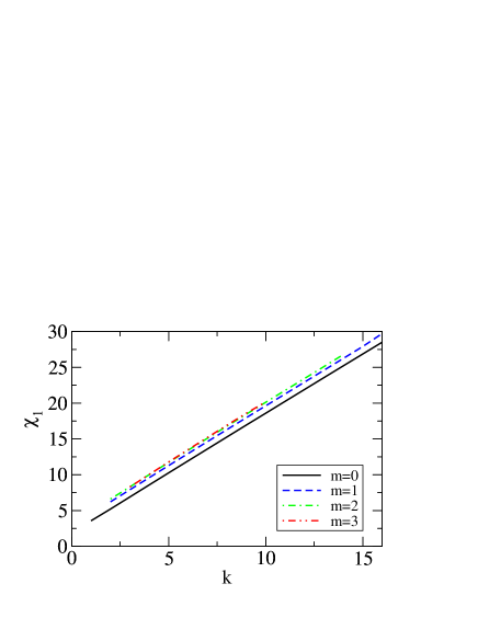
Figure 9: (color online) Approaching the vortex solution. The position of the first node $\chi_{1}$ is shown as a function of the number of digits of precision $k$ in the determining coefficient $a_{0}^{(m)}$ for quantum vortex solutions to the 2D nonlinear Schrödinger equation, as defined in Eq. (59). Observe that all curves are close to parallel and linear in $k$, and as the winding number $m$ increases, the curves converge. Note that all axes are dimensionless.

The reader may ask why obtaining such high precision in the value of $a_{0}^{(m)}$ is desirable. The reason is that each digit of precision brings the solution a few units of $\chi$ closer to the exact vortex solution. In order to obtain a solution which is exactly on the boundary between divergence and non-divergence an infinite number of digits are required. We illustrated this extremely sensitive dependence of the determining coefficient on the number of digits of precision in Fig. 1. Figure 1 depicts three values of $a_{0}$ which approximate $a_{0}^{(m)}$ to $k$ digits of precision, where $k$ is defined by

$$a_{0}=a_{0}^{(m)}(1-10^{-k})\,.$$ (59)

In Eq. (59), a small subtraction is made in the $k$th digit, so that a convergent rather than divergent solution is obtained. In Fig. 1(a), the divergent solution is also depicted for the same value of $k$, with $a_{0}=a_{0}^{(m)}(1+10^{-k})$: i.e., a small addition is made in the $k$th digit. It is in this sense that the vortex solution is a boundary between convergent and divergent solutions.

The figure shows the solution obtained via numerical shooting for $k=16$, 8, and 2 in panels (a), (b), and (c), respectively. A winding number of $m=1$ is assumed. In (b) and (c), the usual Bessel function solution to the two-dimensional linear Schrödinger equation is shown for comparison. One sees that the higher the precision, the further the first node is pushed out towards large values of $\chi$. To move the node to infinity, an infinite number of digits of precision is required. All of the solutions except the divergent one depicted in Fig. 1(a) are examples of ring soliton solutions, as discussed in Sec. IV.

One finds an intriguing relationship between the position of the first node and the number of digits of precision $k$ in the critical determining coefficient $a_{0}^{(m)}$, where $k$ is defined by Eq. (59). In Fig. 9 is shown the position of the first node $\chi_{1}(k)$. One observes that the relationship is linear. For all values of the winding number but $m=0$, the curves lie nearly on top of each other, and all are parallel. Clearly, from Eq. (7), for large $\chi$ the term which depends on $m$ becomes negligible. Note that the use of the special case $m=0$ ensures that, in at least one case, the exact value of $a_{0}^{(m)}$ is known. The best values of $a_{0}^{(m)}$ for $m\neq 0$ are given in Table 2.

A.4 Modified Numerical Method for the Infinite Well

In order to quantize the solutions in an infinite well in two dimensions, one holds the normalization and the cylinder radius to be constant. The form of the wavefunction and the chemical potential can be obtained as follows. One calculates the dependence of the normalization on $a_{0}$ as

$$\int_{0}^{\chi_{j}(a_{0})}d\chi\,\chi[\eta_{m}(\chi)]^{2}=\mathcal{N}_{j}\,,$$ (60)

where $\chi_{j}(a_{0})$ is the distance to the $j$th node in $\eta(\chi)$. As evident in Figs. 1 and 9, a more useful variable to determine the dependence of $\mathcal{N}_{j}$ on $a_{0}$ is the number of digits of precision $k$, as defined by Eq. (59). Note that $k$ is not restricted to an integer value. The value of $k$ also determines $\chi_{j}$. From Eq. (12), the chemical potential scaled to the energy associated with the cylinder radius is

$$\mu_{Rj}\equiv\frac{2MR^{2}}{\hbar^{2}}\mu_{j}=\chi_{j}^{2}\,$$ (61)

where $\mu_{j}$ is the chemical potential for the $(j-1)$th excited state, with $j=1$ giving the ground state. The function $\mu_{Rj}(\mathcal{N}_{j})$ can be calculated from Eqs. (60) and (61). This gives the chemical potential as a function of the atomic interaction strength.

Quantized modes for the infinite spherical well in three dimensions are calculated by similar methods.

References

- (1) L. P. Pitaevskii, Sov. Phys. JETP 13, 451 (1961).
- (2) E. P. Gross, Nuovo Cimento 20, 454 (1961).
- (3) A. L. Fetter, Ann. Phys. 70, 67 (1972).
- (4) R. J. Donnelly, Quantized Vortices in Helium II (Cambridge University Press, New York, 1991).
- (5) M. H. Anderson, et al. Science 269, 198 (1995).
- (6) K. B. Davis et al., Phys. Rev. Lett. 75, 3969 (1995).
- (7) C. C. Bradley, C. A. Sackett, J. J. Tollett, and R. G. Hulet, Phys. Rev. Lett. 75, 1687 (1995).
- (8) C. C. Bradley, C. A. Sackett, and R. G. Hulet, Phys. Rev. A 55, 3951 (1997).
- (9) F. Dalfovo, S. Giorgini, L. P. Pitaevskii, and S. Stringari, Rev. Mod. Phys. 71, 463 (1999).
- (10) A. J. Leggett, Rev. Mod. Phys. 73, 307 (2001).
- (11) M. Greiner, C. A. Regal, and D. S. Jin, Nature 426, 437 (2003).
- (12) S. Jochim et al. Science 302, 2102 (2003).
- (13) M. W. Zwierlein et al. Phys. Rev. Lett. 91, 250401 (2003).
- (14) G. P. Agrawal, Nonlinear Fiber Optics, 2nd ed. (Academic Press, San Diego, 1995).
- (15) M. R. Matthews et al., Phys. Rev. Lett. 83, 2498 (1999).
- (16) K. W. Madison, F. Chevy, W. Wohlleben, and J. Dalibard, Phys. Rev. Lett. 84, 806 (2000).
- (17) S. Burger et al., Phys. Rev. Lett. 83, 5198 (1999).
- (18) J. Denschlag et al., Science 287, 97 (2000).
- (19) P. A. Ruprecht, M. J. Holland, K. Burnett, and M. Edwards, Phys. Rev. A 51, 4704 (1995).
- (20) A. L. Fetter and A. A. Svidzinsky, J. Phys.: Condens. Matter 13, R135 (2001).
- (21) D. L. Feder, C. W. Clark, and B. I. Schneider, Phys. Rev. A 61, 011601(R) (1999).
- (22) J. E. Williams and M. J. Holland, Nature 401, 568 (1999).
- (23) G. Theocharis et al., Phys. Rev. Lett. 90, 120403 (2003).
- (24) Y. S. Kivshar and X. Yang, Phys. Rev. E 49, 1657 (1994).
- (25) W. Dreischuh et al., App. Phys. B 62, 139 (1996).
- (26) D. J. Frantzeskakis and B. A. Malomed, Phys. Lett. A 264, 179 (2000).
- (27) H. E. Nistazakis, D. J. Frantzeskakis, B. A. Malomed, and P. G. Kevrekidis, Phys. Lett. A 285, 157 (2001).
- (28) D. Neshev et al., App. Phys. B 64, 429 (1997).
- (29) A. Dreischuh et al., Phys. Rev. E 66, 066611 (2002).
- (30) In the optics context, ring solitons are not confined by a harmonic trap, which is the primary cause of their instability, as they can expand without limit.
- (31) L. D. Carr, C. W. Clark, and W. P. Reinhardt, Phys. Rev. A 62, 063610 (2000).
- (32) L. D. Carr, C. W. Clark, and W. P. Reinhardt, Phys. Rev. A 62, 063611 (2000).
- (33) L. D. Carr and C. W. Clark, Phys. Rev. Lett. 97, 010403 (2006).
- (34) P. G. Saffman, Vortex Dynamics (Cambridge Univ. Press, New York, 1992).
- (35) D. S. Petrov, M. Holzmann, and G. V. Shlyapnikov, Phys. Rev. Lett. 84, 2551 (2000).
- (36) M. Olshanii, Phys. Rev. Lett. 81, 938 (1998).
- (37) D. S. Petrov, G. V. Shlyapnikov, and J. T. M. Walraven, Phys. Rev. Lett. 85, 3745 (2000).
- (38) L. D. Carr, M. A. Leung, and W. P. Reinhardt, J. Phys. B: At. Mol. Opt. Phys. 33, 3983 (2000).
- (39) K. Bongs et al., Phys. Rev. A 63, 031602 (2001), e-print cond-mat/0007381.
- (40) W. Ketterle, D. S. Durfee, and D. M. Stamper-Kurn, in Bose-Einstein condensation in Atomic Gases, edited by M. Inguscio, S. Stringari, and C. E. Wieman, Proceedings of the International School of Physics “Enrico Fermi” (IOS Press, Amsterdam; Washington, D.C., 1999), pp. 67–176.
- (41) Handbook of Mathematical Functions, edited by M. Abramowitz and I. A. Stegun (National Bureau of Standards, Washington, D. C., 1964).
- (42) R. J. Dodd, J. Research NIST 101, 545 (1996).
- (43) H. Pu, C. K. Law, J. H. Eberly, and N. P. Bigelow, Phys. Rev. A 59, 1533 (1999).
- (44) M. Brack and R. K. Bhaduri, Semiclassical physics (Addison-Wesley, Reading, Massachusetts, 1997).
- (45) L. D. Landau and E. M. Lifshitz, Quantum Mechanics (Non-relativistic Theory) (Pergamon Press, Tarrytown, New York, 1977), Vol. 3.
- (46) R. E. Langer, Phys. Rev. 51, 669 (1937).
- (47) M. V. Berry and K. E. Mount, Rep. Prog. Phys. 35, 315 (1972).
- (48) A. A. Svidzinsky and A. L. Fetter, Phys. Rev. A 58, 3168 (1998).
- (49) L. J. Garay, J. R. Anglin, J. I. Cirac, and P. Zoller, Phys. Rev. A 63, 023611 (2001).
- (50) M. H. Beck, A. Jäckle, G. A. Worth, and H.-D. Meyer, Phys. Rep. 324, 1 (2000).
- (51) C. W. McCurdy, W. A. Isaacs, H.-D. Meyer, and T. N. Rescigno, Phys. Rev. A 67, 042708 (2003).
- (52) W. P. Reinhardt and C. W. Clark, J. Phys. B: At. Mol. Opt. Phys. 30, L785 (1997).
- (53) D. L. Feder et al., Phys. Rev. A 62, 053606 (2000).
- (54) J. J. McClelland and M. R. Scheinfein, J. Opt. Soc. Am. B 8, 1974 (1991).
- (55) J. R. Abo-Shaeer, C. Raman, J. M. Vogels, and W. Ketterle, Science 292, 476 (2001).
- (56) V. Bretin et al., Phys. Rev. Lett. 90, 100403 (2003).
- (57) I. A. Ivonin, V. P. Pavlenko, and H. Persson, Phys. Rev. E 60, 492 (1999).
- (58) A. E. Leanhardt et al., Phys. Rev. Lett. 89, 190403 (2002).
- (59) P. Engels et al., Phys. Rev. Lett. 90, 170405 (2003).
- (60) P. Nozières and D. Pines, The Theory of Quantum Liquids (Addison-Wesley, New York, 1990), Vol. II.
- (61) N. J. Ginsberg, J. Brand, and L. V. Hau, Phys. Rev. Lett. 94, 040403 (2005).
- (62) S. Stock et al., Physical Review Letters 95, 190403 (2005).
- (63) Z. Hadzibabic et al., Nature in press, e-print cond-mat/0605291 (2006).
- (64) Numerical evaluation of the ratios up to indicates that the radius of convergence approaches infinity as , while for the radius of convergence appears to be finite.
- (65) N. G. Berloff, J. Phys. A: Math. Gen. 37, 1617 (2004).
- (66) W. H. Press, S. A. Teukolsky, W. T. Vetterling, and B. P. Flannery, Numerical Recipes in C: The Art of Scientific Computing (Cambridge Univ. Press, Cambridge, U.K., 1993).