Probing Single-Electron Spin Decoherence in Quantum Dots using Charged Excitons

Abstract

We propose to use optical detection of magnetic resonance (ODMR) to measure the decoherence time $T_{2}$ of a single electron spin in a semiconductor quantum dot. The electron is in one of the spin 1/2 states and a circularly polarized laser can only create an optical excitation for one of the electron spin states due to Pauli blocking. An applied electron spin resonance (ESR) field leads to Rabi spin flips and thus to a modulation of the photoluminescence or, alternatively, of the photocurrent. This allows one to measure the ESR linewidth and the coherent Rabi oscillations, from which the electron spin decoherence can be determined. We study different possible schemes for such an ODMR setup, including cw or pulsed laser excitation.

I Introduction

The spin $1/2$ states $|\!\uparrow\rangle$ and $|\!\downarrow\rangle$ of an electron in a semiconductor quantum dot can be used as an implementation of a quantum bit (qubit) spintronics . Due to the rather weak coupling of the spin and orbital degrees of freedom in quantum dots, the electron spin is only weakly interacting with its environment. Still, there is a finite lifetime for spin in these systems, limiting the time during which quantum information can be processed. For single spins, one distinguishes between the two characteristic decay times $T_{1}$ and $T_{2}$. The relaxation of an excited spin state in a magnetic field into the thermal equilibrium occurs with the spin relaxation time $T_{1}$, whereas the spin decoherence time $T_{2}$ is associated with the loss of phase coherence of a single spin that is prepared in a coherent superposition of its eigenstates. Recent experiments with InGaAs and GaAs dots have shown extremely long spin relaxation times up to $T_{1}\approx 1\>\mathrm{ms}$ fujisawa ; hanson ; kouwenhoven . Experimental $T_{2}$ measurements of single electron spins in quantum dots are highly desirable and have not been accomplished so far. It would also be interesting to experimentally verify the theoretical prediction $T_{2}=2T_{1}$ for a quantum dot (with decoherence due to the spin-orbit interaction) golovach .

Coherent control and detection of excitonic states in single quantum dots has been demonstrated in optical experiments gammon1 . Nevertheless, the $T_{2}$ time of a single electron spin in a quantum dot has not yet been measured successfully using optical methods. In this respect, the interaction of the electron and the hole of the exciton imposes a principal difficulty: The electron spin and the hole spin are only decoupled if the hole spin couples stronger to the environment than to the electron spin. However, time-resolved Faraday rotation experiments suggest that there is significant coupling of electron and hole spins in quantum dots guptaT2 . In many other experiments, electron-hole pairs are excited inside the barrier material of a quantum dot heterostructure. After their creation, the carriers diffuse into the dots within typically tens of picoseconds ohnesorge ; raymond . Due to the fast relaxation time of the hole spin in the barrier, electron and hole spins decouple during this time. One would thus expect that in such a setup only the spin decoherence of electrons can be measured, e.g., by the Hanle effect epstein . But this approach has not yet given conclusive results for $T_{2}$. Alternatively, $T_{2}$ can be measured via currents through quantum dots in an ESR field engel:01 ; engel:02 ; martin . However, this requires contacting of the dots with current leads which reduces coherence, while with an optical detection scheme one can also benefit from the high sensitivity of photodetectors.

Optical detection of magnetic resonance (ODMR) has already been applied to measure the coherence of single spins in various systems, including single molecules koehler ; wrachtrup and single nitrogen-vacancy centers in diamond gruber ; jelezko . Recent ODMR experiments on charge-neutral semiconductor quantum dots Lifshitz ; zurauskiene have demonstrated the feasibility of the combination of ESR and optical methods in quantum dot experiments, but have not considered single spin coherence.

In this article, we start by reviewing our recent proposal gywat to measure $T_{2}$ of a single electron spin in a semiconductor quantum dot via ODMR. We also add new results on the detection using photocurrent and on the luminescence intensity autocorrelation function. In Section II, we discuss the states of a negatively charged exciton in a quantum dot. We introduce the Hamiltonian in Section III and describe the dynamics of the ODMR setup with a generalized master equation in Section IV. We show in Section V that the linewidth of the photoluminescence as function of the ESR frequency provides a lower bound on $T_{2}$ gywat . Extending our previous work, we elaborate on the read out via photocurrent in Section VI and discuss in Section VII the autocorrelation function of the luminescence intensity as another possible detection scheme. Further, we identify a regime where $T_{1}$ can be measured optically. We show in Section VIII that electron spin Rabi oscillations can be detected via the photoluminescence if pulsed laser and cw ESR excitation is applied. Using pulsed laser excitation, electron spin precession can be detected with similar schemes, as we discuss in Section IX. We conclude in Section X.

II Negatively Charged Excitons

We consider a quantum dot that confines electrons as well as holes (i.e., a type I dot). We assume that the dot is charged with one single electron. This can be achieved experimentally, e.g., by n-doping cortez , or by electrical injection if the dot is embedded inside a photodiode structure abstreiter2 ; schulhauser . The single-electron state of the dot can be optically excited, creating a negatively charged exciton ($X^{-}$) which consists of two electrons and one hole. In the $X^{-}$ ground state, the two electrons form a spin singlet in the lowest (conduction-band) electron level and the hole occupies the lowest (valence-band) hole level, as shown in recent experiments with InAs dots trion1 ; trion2 and GaAs dots trion3 . Such negatively charged excitons can be used to read out and initialize a single electron spin shabaev . We assume that the lowest heavy hole (hh) dot level (with total angular momentum projection $J_{z}\!=\!\pm 3/2$) and the lowest light hole (lh) dot level (with $J_{z}\!=\!\pm 1/2$) are split by an energy $\delta_{hh-lh}$ and that mixing of hh and lh states is negligible. These conditions are satisfied for several types of quantum dots trion1 ; trion2 ; trion3 ; shabaev ; efrosCdSe ; efros2 . Then, if excitation is restricted to either hh or lh states, the circularly polarized optical transitions $\sigma^{+}$ and $\sigma^{-}$ are unambigously related to one spin polarization of the conduction-band electron because of optical selection rules, see also Fig.  1. Here, we assume a hh ground state for holes.

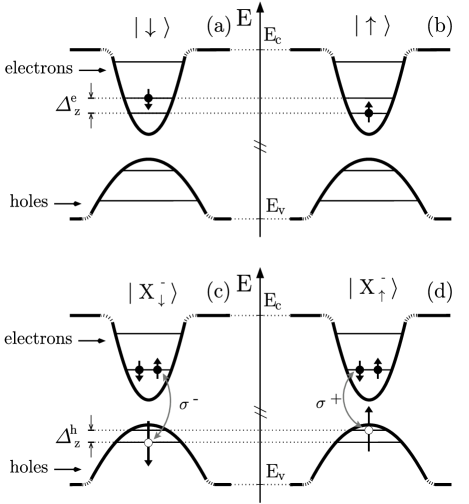
Figure 1: (a)-(d): The states of a single quantum dot in a static magnetic field. The Zeeman splittings are $\Delta_{z}^{e}=g_{e}^{z}{\mu_{\mathrm{B}}}B_{z}$ for the electron and $\Delta_{z}^{h}=g_{hh}^{z}{\mu_{\mathrm{B}}}B_{z}$ for the hole. Coherent transitions occur between (a) and (b) due to an ESR field and between (a) and (c) due to a $\sigma^{-}$-polarized laser field. The grey arrows in (c) and (d) indicate which electron-hole pair couples with the photon field of polarization $\sigma^{\pm}$.

For the proposed ODMR scheme, we consider the following dot states (see also Fig.  1). In the presence of an external static magnetic field, a single electron in the lowest orbital state can be in the spin ground state $|\!\uparrow\rangle$ or in the excited spin state $|\!\downarrow\rangle$. Similarly, an $X^{-}$ in the orbital ground state can either be in the excited spin state $|X_{\downarrow}^{-}\rangle$ or in the spin ground state $|X_{\uparrow}^{-}\rangle$, where the subscripts $\downarrow$ and $\uparrow$ refer to the hh spin. We apply the usual time-inverted notation for hole spins. For simplicity, we have assumed equal signs for the electron and the hh $g$ factors in $z$ direction. Here, we exclude $X^{-}$ states where one electron is in an excited orbital state. The lowest $X^{-}$ state of this type contains an electron triplet and requires an additional energy $\delta\epsilon\approx 40$ meV in InAs dots cortez . This energy difference $\delta\epsilon$ is mainly given by the single-electron level spacing ($\approx 50$ meV fricke ) and the electron-electron exchange interaction. Consequently, the state $|X_{\downarrow}^{-}\rangle$ can be excited resonantly by a circularly polarized laser with a bandwidth lower than $\delta\epsilon$ and $\delta_{hh-lh}$. An ODMR scheme including an $X^{-}$ state with an excited hole is also possible, as we discuss in Section V.

III Hamiltonian

In an ODMR setup with a quantum dot containing a single excess electron, we describe the energy-conserving dynamics with the Hamiltonian

$$H=H_{\mathrm{dot}}+H_{\mathrm{ESR}}+H_{\mathrm{L}}+H_{\mathrm{d-L}},$$ (1)

which couples the three states $|\!\uparrow\rangle$, $|\!\downarrow\rangle$, and $|X_{\downarrow}^{-}\rangle$. Here, $H_{\mathrm{dot}}$ contains the quantum dot potential, the Zeeman energies due to a constant magnetic field $B_{z}$ in the $z$ direction, and the Coulomb interaction of electrons and holes. The dot energy $E_{n}$ is defined by $H_{\mathrm{dot}}|n\rangle=E_{n}|n\rangle$. We set $\hbar=1$ in the following. The electron Zeeman splitting is $\Delta_{z}^{e}=g_{e}^{z}{\mu_{\mathrm{B}}}B_{z}=E_{\downarrow}-E_{\uparrow}$, where $g_{e}^{z}$ is the electron $g$ factor and ${\mu_{\mathrm{B}}}$ is the Bohr magneton. In $B_{z}$, we also include the Overhauser field which could possibly arise from dynamically polarized nuclear spins. The ESR term $H_{\mathrm{ESR}}(t)$ couples the two electron Zeeman levels $|\!\uparrow\rangle$ and $|\!\downarrow\rangle$ via the magnetic field $\mathbf{B}_{\perp}(t)$, which rotates with frequency $\omega_{\mathrm{ESR}}$ in the $xy$ plane. Note that a linearly oscillating magnetic field, $\mathbf{B}_{x}(t)=B_{x}^{0}\cos(\omega_{\mathrm{ESR}}t)\mathbf{\hat{x}}$, can be applied instead of $\mathbf{B}_{\perp}(t)$ sakurai . In the rotating wave approximation, this field leads to the same result as the rotating field with $B_{\perp}\rightarrow B_{x}^{0}/2$. The ESR Rabi frequency is $\Omega_{\mathrm{ESR}}=g_{e}^{\perp}{\mu_{\mathrm{B}}}B_{\perp}$, with in-plane $g$ factor $g_{e}^{\perp}$ (typically, $g_{e}^{\perp}=g_{e}^{z}$). Even if the ESR field is also resonant with the hole Zeeman splitting, the Rabi oscillations of the holes have a negligible effect since the charged exciton states recombine quickly. As an alternative to an ESR field, an oscillating field ${\mu_{\mathrm{B}}}\tensor{\mathbf{g}}\mathbf{B}$ could also be produced using voltage-controlled modulation of the electron $g$-tensor $\tensor{\mathbf{g}}$, which has already been achieved experimentally in quantum wells kato . A $\sigma^{-}$-polarized laser of frequency $\omega_{\mathrm{L}}$ is applied in $z$ direction (typically parallel to $[001]$), with the free laser field Hamiltonian $H_{\mathrm{L}}=\omega_{\mathrm{L}}a_{\mathrm{L}}^{\dagger}a_{\mathrm{L}}$, where $a_{\mathrm{L}}^{(\dagger)}$are photon operators. The optical interaction term $H_{\mathrm{d}-\mathrm{L}}$ describes the coupling of $|\!\downarrow\rangle$ and $|X_{\downarrow}^{-}\rangle$ to the laser field with the complex optical Rabi frequency $\Omega_{\mathrm{L}}$ gywat . We take the coupling to the laser into account in $H_{\mathrm{d-L}}$. Because the laser is circularly polarized, the terms that violate energy conservation vanish due to selection rules. Further, the absorption of a $\sigma^{-}$ photon in the spin ground state $|\!\uparrow\rangle$ is excluded due to Pauli blocking because we assume that the laser bandwidth is smaller than $\delta_{hh-lh}$ and $\delta\epsilon$, as discussed in Section II. Note that the very same scheme can also be applied if the sign of the hole $g$ factor is reversed, since a $\sigma^{+}$ laser field can then be used and all results apply after interchanging $|X_{\downarrow}^{-}\rangle$ and $|X_{\uparrow}^{-}\rangle$. The laser bandwidth and also the temperature can safely exceed the electron Zeeman splitting. Finally, we exclude all multi-photon processes via other levels since they are only relevant to high-intensity laser fields. In this configuration, the $\sigma^{-}$ photon absorption is switched “on” and “off” by the electron spin flips driven by the ESR. We next transform $H$ into the rotating frame with respect to the field frequencies $\omega_{\mathrm{ESR}}$ and $\omega_{\mathrm{L}}$. We introduce the laser detuning $\delta_{\mathrm{L}}=(E_{X\downarrow}-E_{\downarrow})-\omega_{\mathrm{L}}$ and the ESR detuning $\delta_{\mathrm{ESR}}=g_{e}^{z}{\mu_{\mathrm{B}}}B_{z}-\omega_{\mathrm{ESR}}$.

IV Generalized Master Equation

For the dot dynamics including relaxation and decoherence processes, we consider the reduced density matrix for the dot, $\rho={{\mathrm{Tr}}_{\mathrm{R}}\,}\rho_{\mathrm{F}}$. Here, $\rho_{\mathrm{F}}$ is the full density matrix of the dot and its environment (or reservoir), i.e., the unobserved degrees of freedom, and ${{\mathrm{Tr}}_{\mathrm{R}}\,}$ is the trace taken over the reservoir. We take the interaction of the dot states with the ESR and the laser fields exactly into account using the Hamiltonian [Eq. (1)] in the rotating frame. With a generalized master equation in the Lindblad form, we take the coupling with the environment (radiation field, nuclear spins, phonons, spin-orbit interaction, etc.) into account with phenomenological rates. We use the rates $W_{nm}\equiv W_{n\leftarrow m}$ for the incoherent transitions from state $|m\rangle$ to $|n\rangle$ and the rates $V_{nm}$ for the decay of the corresponding off-diagonal matrix elements of $\rho$. These decoherence rates $V_{nm}$ have the structure $V_{nm}=\frac{1}{2}\sum_{k}\left(W_{kn}+W_{km}\right)+V_{n}+V_{m},$ where the rate $V_{n}+V_{m}$ is usually called the pure decoherence rate. Further, the electron spin relaxation time is $T_{1}=\left(W_{{\uparrow\downarrow}}+W_{{\downarrow\uparrow}}\right)^{-1}$, with spin flip rates $W_{{\uparrow\downarrow}},W_{{\downarrow\uparrow}}$. (In Section V below, we point out a method to measure $T_{1}$ in a similar setup as discussed here.) In the absence of the ESR field and the laser field, the off-diagonal matrix elements of the electron spin decay with the (intrinsic) single-spin decoherence rate $V_{{\downarrow\uparrow}}=\frac{1}{2}(W_{{\uparrow\downarrow}}+W_{{\downarrow\uparrow}})+V_{\uparrow}+V_{\downarrow}=1/T_{2}$. Further, the linewidth of the optical $\sigma^{-}$ transition is denoted by $V_{\mathrm{X}}=V_{X\downarrow,\downarrow}$. We use the notation $\rho_{n}=\langle n|\rho|n\rangle$ and $\rho_{n,m}=\langle n|\rho|m\rangle$ for the matrix elements of $\rho$. In the rotated basis $|\!\uparrow\rangle$, $|\!\downarrow\rangle$, $|X_{\uparrow}^{-}\rangle$, $|X_{\downarrow}^{-}\rangle$, the generalized master equation is given by $\dot{\rho}=\mathcal{M}\rho$, where $\mathcal{M}$ is a superoperator. Explicitly,

$${{\dot{\rho}_{\uparrow}}} = \Omega_{\mathrm{ESR}}{\textrm{Im}}\rho_{\downarrow,\uparrow}\!+\!W_{\mathrm{em}}\rho_{X\uparrow}\!+\!W_{{\uparrow\downarrow}}{\rho_{\downarrow}}\!-\!W_{{\downarrow\uparrow}}{\rho_{\uparrow}},$$ (2)

$${{\dot{\rho}_{\downarrow}}} = -\Omega_{\mathrm{ESR}}{\textrm{Im}}\rho_{\downarrow,\uparrow}+{\textrm{Im}}(\Omega_{\mathrm{L}}^{*}\rho_{X\downarrow,\downarrow})+W_{\mathrm{em}}\,\rho_{X\downarrow}$$ (3)

$$+W_{{\downarrow\uparrow}}\,{\rho_{\uparrow}}-W_{{\uparrow\downarrow}}\,{\rho_{\downarrow}},$$

$$\dot{\rho}_{X\downarrow} = -{\textrm{Im}}(\Omega_{\mathrm{L}}^{*}\rho_{X\downarrow,\downarrow})+W_{X\downarrow,X\uparrow}\,\rho_{X\uparrow}$$ (4)

$$-\left(W_{\mathrm{em}}+W_{X\uparrow,X\downarrow}\right)\rho_{X\downarrow},$$

$$\dot{\rho}_{X\uparrow} = W_{X\uparrow,X\downarrow}\,\rho_{X\downarrow}-\left(W_{\mathrm{em}}+W_{X\downarrow,X\uparrow}\right)\rho_{X\uparrow},$$ (5)

$${{\dot{\rho}_{\downarrow,\uparrow}}} = \frac{i}{2}\Omega_{\mathrm{ESR}}\left({\rho_{\downarrow}}-{\rho_{\uparrow}}\right)-\frac{i}{2}\Omega_{\mathrm{L}}^{*}\rho_{X\downarrow,\uparrow}$$ (6)

$$-\left(i\delta_{\mathrm{ESR}}+T_{2}^{-1}\right)\,\rho_{\downarrow,\uparrow},$$

$$\dot{\rho}_{X\downarrow,\uparrow} = \frac{i}{2}\Omega_{\mathrm{ESR}}\,\rho_{X\downarrow,\downarrow}-\frac{i}{2}\Omega_{\mathrm{L}}\rho_{\downarrow,\uparrow}$$ (7)

$$-[i(\delta_{\mathrm{ESR}}+\delta_{\mathrm{L}})+V_{X\downarrow,\uparrow}]\,\rho_{X\downarrow,\uparrow},$$

$$\dot{\rho}_{X\downarrow,\downarrow} = \frac{i}{2}\Omega_{\mathrm{ESR}}\rho_{X\downarrow,\uparrow}-\frac{i}{2}\Omega_{\mathrm{L}}({\rho_{\downarrow}}-\rho_{X\downarrow})$$ (8)

$$-(i\delta_{\mathrm{L}}+V_{\mathrm{X}})\rho_{X\downarrow,\downarrow}.$$

The remaining (off-diagonal) matrix elements of $\rho$ are decoupled from these equations and are not further important here.

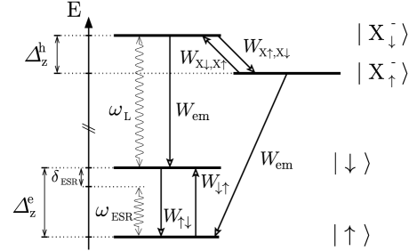
Figure 2: Level scheme of the four states shown in Fig. 1. Wavy arrows describe the transitions driven by the ESR field and the laser field with frequencies $\omega_{\mathrm{ESR}}$ and $\omega_{\mathrm{L}}$, respectively. The corresponding Rabi frequencies are $\Omega_{\mathrm{ESR}}$ and $|\Omega_{\mathrm{L}}|$. A detuning $\delta_{\mathrm{ESR}}=\Delta_{z}^{e}-\omega_{\mathrm{ESR}}$ is shown for the ESR field, with Zeeman splitting $\Delta_{z}^{e}$. Incoherent transitions are shown with arrows and occur at rates $W_{nm}$. We consider $W_{\downarrow,X\downarrow}=W_{\uparrow,X\uparrow}=:W_{\mathrm{em}}$.

V ESR Linewidth in the Photoluminescence

We now calculate the stationary photoluminescence for a cw ESR field and a cw laser field. For this, we evaluate the stationary density matrix $\bar{\rho}$, which satisfies $\dot{\bar{\rho}}=0$. We introduce the effective rate

$$W_{\mathrm{L}}=\frac{|\Omega_{\mathrm{L}}|^{2}}{2}\>\frac{V_{\mathrm{X}}}{V_{\mathrm{X}}^{2}+\delta_{\mathrm{L}}^{2}}$$ (9)

for the optical excitation, which takes its maximum value $W_{\mathrm{L}}^{\mathrm{max}}$ for $\delta_{\mathrm{L}}=0$. We first solve $\dot{\bar{\rho}}_{X\downarrow,\uparrow}=0$. We find that the coupling to the laser field produces an additional decoherence channel to the electron spin. We thus obtain a renormalized spin decoherence rate $V_{\mathrm{ESR}}$, which satisfies

$$V_{\mathrm{ESR}}\leq\frac{1}{T_{2}}+\frac{|\Omega_{\mathrm{L}}|^{2}}{4V_{X\downarrow,\uparrow}}\approx\frac{1}{T_{2}}+\frac{1}{2}W_{\mathrm{L}}^{\mathrm{max}}.$$ (10)

Similarly, the ESR detuning $\delta_{\mathrm{ESR}}$ is also renormalized,

$$\tilde{\delta}_{\mathrm{ESR}}\geq\delta_{\mathrm{ESR}}\left[1-\frac{|\Omega_{\mathrm{L}}|^{2}}{\left(W_{\mathrm{em}}+W_{X\uparrow,X\downarrow}\right)^{2}}\right].$$ (11)

We assume that these renormalizations and $\delta_{\mathrm{L}}$ are small compared to the optical linewidth $V_{\mathrm{X}}$, i.e., $W_{\mathrm{L}}^{\mathrm{max}},\,|\tilde{\delta}_{\mathrm{ESR}}-\delta_{\mathrm{ESR}}|<V_{\mathrm{X}}$. Further, if both transitions are near resonance, $\delta_{\mathrm{L}}\lesssim V_{\mathrm{X}}$ and $|\tilde{\delta}_{\mathrm{ESR}}|\lesssim V_{\mathrm{ESR}}$, no additional terms appear in the renormalized master equation. We then solve $\dot{\bar{\rho}}_{X\downarrow,\downarrow}=0$ and $\dot{\bar{\rho}}_{\downarrow,\uparrow}=0$ and introduce the effective Rabi spin-flip rate

$$W_{\mathrm{ESR}}=\frac{\Omega_{\mathrm{ESR}}^{2}}{2}\>\frac{V_{\mathrm{ESR}}}{V_{\mathrm{ESR}}^{2}+{\tilde{\delta}_{\mathrm{ESR}}}^{2}},$$ (12)

which together with $W_{\mathrm{L}}$ eliminates the parameters $\Omega_{\mathrm{L}}$, $V_{\mathrm{X}}$, $\delta_{\mathrm{L}}$, $\Omega_{\mathrm{ESR}}$, $V_{\mathrm{ESR}}$, and $\tilde{\delta}_{\mathrm{ESR}}$ in the remaining equations for the diagonal elements of $\rho$. Further, these now contain the total spin flip rates $\tilde{W}_{{\uparrow\downarrow}}=W_{{\uparrow\downarrow}}+W_{\mathrm{ESR}}$ and $\tilde{W}_{{\downarrow\uparrow}}=W_{{\downarrow\uparrow}}+W_{\mathrm{ESR}}$. We obtain the stationary solution

$$\bar{\rho}_{\uparrow} = \eta W_{\mathrm{L}}\,W_{\mathrm{em}}\,W_{X\uparrow,X\downarrow}+\eta\tilde{W}_{{\uparrow\downarrow}}\,W_{\mathrm{em}}\,W_{X\uparrow,X\downarrow}$$ (13)

$$+\eta\tilde{W}_{{\uparrow\downarrow}}\left(W_{\mathrm{L}}+W_{\mathrm{em}}\right)\left(W_{\mathrm{em}}+W_{X\downarrow,X\uparrow}\right),$$

$$\bar{\rho}_{\downarrow} = \eta\tilde{W}_{{\downarrow\uparrow}}\,\left(W_{\mathrm{L}}+W_{\mathrm{em}}\right)\left(W_{\mathrm{em}}+W_{X\downarrow,X\uparrow}\right)$$ (14)

$$+\eta\tilde{W}_{{\downarrow\uparrow}}\,W_{\mathrm{em}}\,W_{X\uparrow,X\downarrow},$$

$$\bar{\rho}_{X\downarrow} = \eta W_{\mathrm{L}}\,\tilde{W}_{{\downarrow\uparrow}}\,\left(W_{\mathrm{em}}+W_{X\downarrow,X\uparrow}\right),$$ (15)

$$\bar{\rho}_{X\uparrow} = \eta W_{\mathrm{L}}\,\tilde{W}_{{\downarrow\uparrow}}\,W_{X\uparrow,X\downarrow},$$ (16)

where the normalization factor $\eta$ is chosen such that $\sum_{n}\rho_{n}=1$. Comparing the expressions for $\bar{\rho}_{\uparrow}$ and $\bar{\rho}_{\downarrow}$ above, we see that $\bar{\rho}_{\uparrow}\geq\bar{\rho}_{\downarrow}$ is satisfied for $W_{{\uparrow\downarrow}}\geq W_{{\downarrow\uparrow}}$. This electron spin polarization is due to the hole spin relaxation channel, analogous as in an optical pumping scheme. A hole spin flip corresponds to leakage out of the states that are driven by the external fields. Since the dynamics due to the ESR is much slower than the optical recombination, there is an increased population of the state $|\!\uparrow\rangle$.

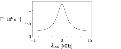
Figure 3: The stationary photoluminescence rate $\Gamma$ as a function of the ESR detuning $\tilde{\delta}_{\mathrm{ESR}}$. As described in the text, $\Gamma$ is a Lorentzian and its linewidth $w$ gives an upper bound for $2/T_{2}$. Here, we use $g_{e}=0.5$, $B_{\perp}=1\>\mathrm{G}$, $T_{2}=100\>\mathrm{ns}$, $W_{{\uparrow\downarrow}}=W_{{\downarrow\uparrow}}=(20\>\mathrm{\mu s})^{-1}$, $W_{\mathrm{em}}=10^{9}\>\mathrm{s^{-1}}$, $W_{X\uparrow,X\downarrow}=W_{X\downarrow,X\uparrow}=W_{\mathrm{em}}/2$, $\delta_{\mathrm{L}}=0$, $V_{X\downarrow,\uparrow}=V_{\mathrm{X}}=(W_{\mathrm{em}}+W_{X\uparrow,X\downarrow})/2$, and $\Omega_{\mathrm{L}}=2\Omega_{\mathrm{ESR}}\sqrt{T_{2}V_{\mathrm{X}}}$. With these parameters, $W_{\mathrm{L}}\lesssim T_{2}^{-1}\lesssim V_{\mathrm{ESR}}$ is satisfied.

The stationary photoluminescence $\Gamma=\Gamma^{-}+\Gamma^{+}$ consists of a $\sigma^{-}$ and a $\sigma^{+}$ polarized contribution, $\Gamma^{-}=W_{\mathrm{em}}\bar{\rho}_{X\downarrow}$ and $\Gamma^{+}=W_{\mathrm{em}}\bar{\rho}_{X\uparrow}$, respectively. We find that the rates $\Gamma^{-}$ and $\Gamma^{+}$ are proportional to $W_{\mathrm{ESR}}/(\gamma+W_{\mathrm{ESR}})$ for a given $\gamma$, up to a constant background which is negligible for $W_{{\downarrow\uparrow}}<W_{\mathrm{ESR}}$. In particular, the total emission rate $\Gamma=\Gamma^{-}+\Gamma^{+}$ as function of $\tilde{\delta}_{\mathrm{ESR}}$ is a Lorentzian with linewidth

$$w=2\,V_{\mathrm{ESR}}\sqrt{1+\frac{W_{\mathrm{ESR}}^{\mathrm{max}}}{\gamma}},$$ (17)

see also Fig.  3. By analyzing the expression for $\gamma$, we find the relevant parameter regime with the inequality

$$w \leq 2V_{\mathrm{ESR}}\Bigg{[}1\!+\!\frac{2W_{\mathrm{ESR}}^{\mathrm{max}}}{W_{\mathrm{L}}}\left(1\!+\!\frac{W_{\mathrm{em}}}{W_{\mathrm{r}}}\!+\!\frac{W_{X\downarrow,X\uparrow}}{W_{\mathrm{r}}}\right)\!$$ (18)

$$+\!\frac{3W_{\mathrm{ESR}}^{\mathrm{max}}}{W_{\mathrm{r}}}\!+\!\frac{W_{\mathrm{ESR}}^{\mathrm{max}}}{W_{\mathrm{em}}}\left(1\!+\!\frac{3\,W_{X\downarrow,X\uparrow}}{W_{\mathrm{r}}}\right)\Bigg{]}^{1/2}\!\!\!\!\!\!\!\!,$$

which saturates for vanishing spin flip rates $W_{{\downarrow\uparrow}}$ and $W_{{\uparrow\downarrow}}$. Here, we have introduced the rate $W_{\mathrm{r}}=W_{X\uparrow,X\downarrow}+W_{{\uparrow\downarrow}}\left(1+W_{\mathrm{em}}/W_{\mathrm{L}}\right)$ which describes different relaxation channels that lead to the ground state $|\!\uparrow\rangle$. These correspond to “switching off” the laser excitations because of Pauli blocking. The linewidth $w$ thus provides a lower bound for $T_{2}$:

$$T_{2}\geq V_{\mathrm{ESR}}^{-1}\geq\frac{2}{w}.$$ (19)

Here, the second inequality saturates when the expression in brackets in Eq. (18) becomes close to 1 (e.g., for efficient hole spin relaxation Flissikowski ; woods $W_{\mathrm{r}}$ is large and $w\approx 2\,V_{\mathrm{ESR}}$). For the first inequality, $T_{2}\approx V_{\mathrm{ESR}}^{-1}$ for $W_{\mathrm{L}}^{\mathrm{max}}<1/T_{2}$, see Eq. (10). To check our analytical approximation for $\Gamma$, we have solved the generalized master equation numerically using the parameters given in the caption of Fig.  3. Comparing the two results for $\Gamma$, we find that the relative difference is less than $0.2\>\%$.

Due to possible imperfections in the ODMR scheme described above, e.g., due to mixing of hh and lh states or due to a small contribution of the $\sigma^{+}$ polarization in the laser light, there can be a small probability that the Pauli blocking of absorption is somewhat lifted and the state $|\!\uparrow\rangle$ can be optically excited. We describe this process with the effective rate $W_{\mathrm{L},\uparrow}$. It leads to an additional linewidth broadening, similar to the one described with Eq. (18). We find that this effect is small if $W_{\mathrm{L},\uparrow}<W_{\mathrm{ESR}}$.

The setup discussed in this section combines optical excitation and detection at the same wavelength. The laser stray light is an undesirable background here and its detection can be avoided, e.g., by using a polarization filter and by measuring only $\Gamma^{+}$. The laser could also be distinguished from $\Gamma^{-}$ if two-photon excitation is applied, which is, e.g., possible with excitons in II-VI (e.g., CdSe cdse2phot or CdS cds2phot ) and I-VII (e.g., CuCl cucl2phot ) semiconductor nanocrystals. As another alternative, the optical excitation could be tuned to an excited hole state (hh or lh) grundmann , possibly with a reversal of laser polarization. Using a pulsed laser would enable the distinction between luminescence and laser light by time-gated detection. See also Section VIII for another detection scheme with a pulsed laser. Another option is to detect the resonant absorption instead of the photoluminescence, using an optical transmission setup hoegele . Finally, one can also measure the photocurrent photocurrent ; photocurrent2 instead of the photoluminescence, which we discuss in the following section.

VI Read Out via Photocurrent

As an alternative to photon detection, the presence of a charged exciton $X^{-}$ on the dot can also be read out via an electric current (the so-called photocurrent) photocurrent ; photocurrent2 . Here, a strong electric field is applied across the quantum dot, and one electron and one hole tunnel out of the dot into two adjacent current leads. Thus, the total charge $e$ is transported through the dot per optical excitation, where $e$ is the elementary charge. Because the tunneling process is spin-independent, the remaining electron on the dot has equal probabilities to be in state $|\!\uparrow\rangle$ or in state $|\!\downarrow\rangle$, in contrast to the read out using photoluminescence. We now calculate the stationary photocurrent. For this, we apply a generalized master equation description, similarly as in Section IV for the photoluminescence. We introduce phenomenological photocurrent rates $W_{\mathrm{pc}}$ as shown in Fig. 4. For strong tunneling ($W_{\mathrm{pc}}>W_{\mathrm{em}}$), optical recombination is negligible and the $X^{-}$ are predominantly detected via the photocurrent. The generalized master equation is then given by

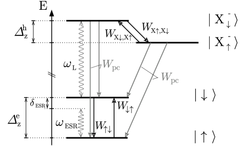
Figure 4: Scheme of the transitions for the read out via photocurrent. The tunneling of the electron and the hole out of the dot is spin-independent. Therefore, transitions occuring at a rate $W_{\mathrm{pc}}$ lead from the charged exciton states $|X_{\uparrow}^{-}\rangle$, $|X_{\downarrow}^{-}\rangle$ to both spin states $|\!\uparrow\rangle$ and $|\!\downarrow\rangle$, respectively. The remaining symbols are defined as in Fig. 2.

$${{\dot{\rho}_{\uparrow}}} = \Omega_{\mathrm{ESR}}{\textrm{Im}}\rho_{\downarrow,\uparrow}\!+\!W_{\mathrm{pc}}(\rho_{X\uparrow}+\rho_{X\downarrow})\!$$ (20)

$$+\!W_{{\uparrow\downarrow}}{\rho_{\downarrow}}\!-\!W_{{\downarrow\uparrow}}{\rho_{\uparrow}},$$

$${{\dot{\rho}_{\downarrow}}} = -\Omega_{\mathrm{ESR}}{\textrm{Im}}\rho_{\downarrow,\uparrow}+{\textrm{Im}}(\Omega_{\mathrm{L}}^{*}\rho_{X\downarrow,\downarrow})+W_{{\downarrow\uparrow}}\,{\rho_{\uparrow}}$$ (21)

$$+W_{\mathrm{pc}}(\rho_{X\uparrow}+\rho_{X\downarrow})-W_{{\uparrow\downarrow}}\,{\rho_{\downarrow}},$$

$$\dot{\rho}_{X\downarrow} = -{\textrm{Im}}(\Omega_{\mathrm{L}}^{*}\rho_{X\downarrow,\downarrow})+W_{X\downarrow,X\uparrow}\,\rho_{X\uparrow}$$ (22)

$$-\left(2W_{\mathrm{pc}}+W_{X\uparrow,X\downarrow}\right)\rho_{X\downarrow},$$

$$\dot{\rho}_{X\uparrow} = W_{X\uparrow,X\downarrow}\,\rho_{X\downarrow}-\left(2W_{\mathrm{pc}}+W_{X\downarrow,X\uparrow}\right)\rho_{X\uparrow},$$ (23)

$${{\dot{\rho}_{\downarrow,\uparrow}}} = \frac{i}{2}\Omega_{\mathrm{ESR}}\left({\rho_{\downarrow}}-{\rho_{\uparrow}}\right)-\frac{i}{2}\Omega_{\mathrm{L}}^{*}\rho_{X\downarrow,\uparrow}$$ (24)

$$-\left(i\delta_{\mathrm{ESR}}+T_{2}^{-1}\right)\,\rho_{\downarrow,\uparrow},$$

$$\dot{\rho}_{X\downarrow,\uparrow} = \frac{i}{2}\Omega_{\mathrm{ESR}}\,\rho_{X\downarrow,\downarrow}-\frac{i}{2}\Omega_{\mathrm{L}}\rho_{\downarrow,\uparrow}$$ (25)

$$-[i(\delta_{\mathrm{ESR}}+\delta_{\mathrm{L}})+V_{X\downarrow,\uparrow}]\,\rho_{X\downarrow,\uparrow},$$

$$\dot{\rho}_{X\downarrow,\downarrow} = \frac{i}{2}\Omega_{\mathrm{ESR}}\rho_{X\downarrow,\uparrow}-\frac{i}{2}\Omega_{\mathrm{L}}({\rho_{\downarrow}}-\rho_{X\downarrow})$$ (26)

$$-(i\delta_{\mathrm{L}}+V_{\mathrm{X}})\rho_{X\downarrow,\downarrow}.$$

Note that in the previous expressions for $V_{\mathrm{X}}$ and $V_{X\downarrow,\uparrow}$, the relaxation rate $W_{\mathrm{em}}$ is now replaced by $\tilde{W}_{\mathrm{pc}}=2W_{\mathrm{pc}}$. We then obtain for the stationary solution

$$\bar{\rho}_{\uparrow} = \tilde{\eta}W_{\mathrm{L}}\tilde{W}_{\mathrm{pc}}\!+\!\tilde{\eta}\tilde{W}_{{\uparrow\downarrow}}\,\tilde{W}_{\mathrm{pc}}\!+\!\tilde{\eta}\tilde{W}_{{\uparrow\downarrow}}\!\!\left(\!W_{\mathrm{L}}\!+\!\tilde{W}_{\mathrm{pc}}\!\right),$$ (27)

$$\bar{\rho}_{\downarrow} = \tilde{\eta}\tilde{W}_{{\downarrow\uparrow}}\,\left(W_{\mathrm{L}}+\tilde{W}_{\mathrm{pc}}\right)+\tilde{\eta}\tilde{W}_{{\downarrow\uparrow}}\,\tilde{W}_{\mathrm{pc}},$$ (28)

$$\bar{\rho}_{X\downarrow} = \tilde{\eta}W_{\mathrm{L}}\,\tilde{W}_{{\downarrow\uparrow}},$$ (29)

$$\bar{\rho}_{X\uparrow} = \tilde{\eta}W_{\mathrm{L}}\,\tilde{W}_{{\downarrow\uparrow}}.$$ (30)

Here, $\tilde{\eta}$ is a normalization factor such that $\sum_{n}\rho_{n}=1$. The photocurrent $I_{\mathrm{pc}}=e\tilde{W}_{\mathrm{pc}}(\bar{\rho}_{X\downarrow}+\bar{\rho}_{X\uparrow})$ is a Lorentzian as a function of the ESR detuning $\tilde{\delta}_{\mathrm{ESR}}$. The linewidth is bound by the inequality

$$w \leq 2\,V_{\mathrm{ESR}}\,\Bigg{[}1+4W_{\mathrm{ESR}}^{\mathrm{max}}\,\left(\frac{1}{W_{\mathrm{L}}}+\frac{1}{\tilde{W}_{\mathrm{pc}}}\right)\Bigg{]}^{1/2},$$ (31)

where the right hand side is a smaller upper bound for $w$ than the one obtained for the photoluminescence [Eq. (18)]. This can be understood by noting that above result for the photocurrent can also be obtained from the expression for the stationary photoluminescence (see Section V) by replacing $W_{\mathrm{em}}\rightarrow\tilde{W}_{\mathrm{pc}}$ and in the limit $W_{X\uparrow,X\downarrow},\,W_{X\downarrow,X\uparrow}\rightarrow\infty$.

VII Luminescence Intensity Autocorrelation Function

The luminescence intensity autocorrelation function $\left\langle I(t)I(t+\tau)\right\rangle$ has recently been used in experiments to demonstrate the suitability of single quantum dots for single-photon sources michler ; zwiller . We discuss here that electron spin Rabi oscillations can be detected via $\left\langle I(t)I(t+\tau)\right\rangle$. For this, we assume that the laser polarization is changed to $\sigma^{+}$. At low temperatures ($kT<g_{hh}^{z}{\mu_{\mathrm{B}}}B_{z}$, where $k$ is the Boltzmann constant), excitations of the hole spin are negligible since $W_{X\downarrow,X\uparrow}\ll W_{\mathrm{em}}$. Then, the energetically highest state $|X_{\downarrow}^{-}\rangle$ is decoupled from the three-level system $|\!\uparrow\rangle$, $|\!\downarrow\rangle$, and $|X_{\uparrow}^{-}\rangle$, cf.  Fig. 5. After emission of a $\sigma^{+}$ photon, the dot is in the state $|\!\uparrow\rangle$. For the transitions shown in Fig. 5, we derive a generalized master equation similarly as Eqs. (2)-(8) were derived according to Fig. 2. We model the time evolution of the dot state $|\!\uparrow\rangle$ in lowest order in $W_{\mathrm{L}}$ and obtain the probability to be in the final state $|X_{\uparrow}^{-}\rangle$ after some time $\tau$. We consider the regime $W_{\mathrm{L}}\leq V_{\mathrm{ESR}}$ and $V_{\mathrm{ESR}}\ll\Omega_{\mathrm{ESR}}<W_{\mathrm{em}}$ and obtain for the luminescence intensity autocorrelation function

$$\left\langle I(t)I(t+\tau)\right\rangle=W_{\mathrm{L}}^{2}\bar{\rho}_{\uparrow}^{\,2}P_{\uparrow}(\tau)+o(W_{\mathrm{L}}^{3}).$$ (32)

Here, $I(t)$ is the $\sigma^{+}$ luminescence intensity, $\bar{\rho}_{\uparrow}\approx\tilde{W}_{{\uparrow\downarrow}}/(\tilde{W}_{{\uparrow\downarrow}}+\tilde{W}_{{\downarrow\uparrow}})$ is the stationary occupation of $|\!\uparrow\rangle$, and $P_{\uparrow}(\tau)$ is the conditional probability to be again in the state $|\!\uparrow\rangle$ after the time $t+\tau$ if the state was $|\!\uparrow\rangle$ at time $t$. For $\delta_{\mathrm{ESR}}=0$ and $W_{{\uparrow\downarrow}}=W_{{\downarrow\uparrow}}$, we find $P_{\uparrow}(\tau)\approx 1/2+(1/2)\exp\left[-(\tau/2)\left(1/T_{2}+1/T_{1}\right)\right]\cos(\Omega_{\mathrm{ESR}}\tau)$. Thus, the inverse decay rate of the detected oscillations in $\left\langle I(t)I(t+\tau)\right\rangle$ [Eq. (32)] gives a lower bound on $2T_{2}$.

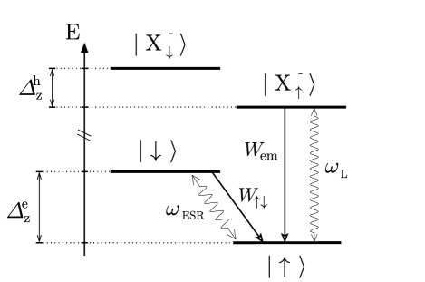
Figure 5: Scheme of the transitions if an ESR field and a $\sigma^{+}$ polarized laser field are applied. As described in the text, $|X_{\downarrow}^{-}\rangle$ is decoupled from the other three states at low temperatures. In this setup, the luminescence intensity autocorrelation function $\left\langle I(t)I(t+\tau)\right\rangle$ can be used to detect the decay of spin oscillations. Further, for a larger laser intensity, $T_{1}$ can be measured as explained in Section VII.

To conclude this section, we briefly point out that the single-spin relaxation time $T_{1}$ can be measured via a similar double resonance scheme as discussed for $\left\langle I(t)I(t+\tau)\right\rangle$ above. This can be done in the regime $\Omega_{\mathrm{L}},\,W_{\mathrm{em}}\gg\Omega_{\mathrm{ESR}},\,W_{{\uparrow\downarrow}}$, i.e., we require a larger intensity of the $\sigma^{+}$ laser as considered for the $T_{2}$ measurement. Then, the system is predominantly driven by the laser field. Occasionally, the ESR field excites the electron spin and interrupts the optical excitations. After relaxation of the spin, the laser again acts on the dot and gives rise to photoluminescence. The mean time of photoluminescence interruptions due to ESR excitation is thus given by $T_{1}$, similarly as for a single atom kimble .

VIII Spin Rabi Oscillations via Photoluminescence

The photoluminescence $\Gamma$ can be measured as a function of the pulse repetition time $\tau_{\mathrm{rep}}$ of a pulsed laser while keeping $\delta_{\mathrm{ESR}}$ constant. We again consider cw ESR and choose $\sigma^{-}$ for the laser polarization, while the previous restrictions on the laser bandwidth still apply (see Section II). Since excessive population is trapped in the state $|\!\uparrow\rangle$ during a laser pulse due to hole spin flips and subsequent emission of a photon, the dot is preferably in the state $|\!\uparrow\rangle$ (rather than $|\!\downarrow\rangle$) at the end of a laser pulse. During the “off” time of the laser between two pulses, the ESR field rotates the electron spin. The next laser pulse then reads out the spin state $|\!\downarrow\rangle$. Thus, as a function of $\tau_{\mathrm{rep}}$, the spin Rabi oscillations can be observed in the photoluminescence (similarly as in $\left\langle I(t)I(t+\tau)\right\rangle$), see Fig.  6. To model the pulsed laser excitation, we consider square pulses of length $\Delta t$, for simplicity. In the generalized master equation ${{\dot{\rho}}}(t)=\mathcal{M}(t)\rho(t)$, we write $\mathcal{M}(t)=\mathcal{M}_{\mathrm{L}}$ [where $\mathcal{M}_{\mathrm{L}}$ is defined via Eqs. (2) - (8)] during a laser pulse and $\mathcal{M}(t)=\mathcal{M}_{0}$ otherwise, setting $\Omega_{\mathrm{L}}=0$. We obtain the steady-state density matrix $\rho_{\infty}$ of the dot state just after the pulse from $U_{p}\rho_{\infty}=\rho_{\infty}$, where $U_{p}=\exp(\mathcal{M}_{\mathrm{L}}\Delta t)\exp[\mathcal{M}_{0}(\tau_{\mathrm{rep}}-\Delta t)]$ describes the time evolution of $\rho$ during $\tau_{\mathrm{rep}}$.

Figure 6: The average number $N=\Gamma\tau_{\mathrm{rep}}$ of photons emitted per period $\tau_{\mathrm{rep}}$ as a function of the laser pulse repetition time $\tau_{\mathrm{rep}}$. In (a), $\pi$ pulses are used for the laser with $\Delta t=5\,\mathrm{ps}$ and $\Omega_{\mathrm{L}}=\pi/\Delta t$. In (b), $N$ is shown for pulses with $\Delta t=20\,\mathrm{ns}$ and $\Omega_{\mathrm{L}}=\pi/(500\,\mathrm{ps})$. We have set $\delta_{\mathrm{ESR}}=0$. The other parameters are the same as in Fig. 3. The decay of the oscillation depends on $T_{2}$.

The steady-state photoluminescence is now calculated by $\Gamma=W_{\mathrm{em}}\overline{(\rho_{X\downarrow}+\rho_{X\uparrow})}$, where the bar symbolizes time averaging over many periods $\tau_{\mathrm{rep}}$. If the laser pulse duration is longer than the lifetime of a negatively charged exciton, $\Delta t>W_{\mathrm{em}}^{-1}$ (and not shorter than an optical $\pi$ pulse), the spin oscillations become more pronounced, see Fig. 6 (b). This is because after an optical recombination of the state $|X_{\downarrow}^{-}\rangle$, the laser pulse is still on and excites the state $|\!\downarrow\rangle$ again to $|X_{\downarrow}^{-}\rangle$. This iterated excitation increases the total probability of a hole spin flip during a laser pulse and therefore the total population trapped in the state $|\!\uparrow\rangle$.

IX Spin Precession via Photoluminescence

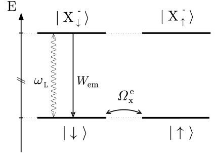
Figure 7: Level scheme of the spin states in the $z$ direction in the Voigt geometry. Optical transitions with circular polarization occur vertically in this scheme. The transverse magnetic field $B_{x}$ leads to spin precession, i.e., periodic oscillations between the spin states $|\!\uparrow\rangle$ and $|\!\downarrow\rangle$ at a frequency $\Omega_{x}^{e}=g_{e}^{x}{\mu_{\mathrm{B}}}B_{x}/2$. In this figure, we do not illustrate the precession of hole spins, assuming that $W_{\mathrm{em}}\gg\Omega_{x}^{h}=g_{h}^{x}{\mu_{\mathrm{B}}}B_{x}/2$.

Similar to Rabi oscillations, the precession of a single electron spin in a static magnetic field can also be observed if pulsed laser excitation is applied to a quantum dot charged with a single excess electron. For this, we consider the Voigt geometry, i.e., a static magnetic field is applied in a direction $x$, transverse to the laser beam direction $z$. We again assume circular polarization of the laser. Consequently, the optical transitions are between the spin states along the quantization axis in $z$ direction, see Fig. 7. For low temperatures woods and for $W_{\mathrm{em}}\gg\Omega_{x}^{h}=g_{h}^{x}{\mu_{\mathrm{B}}}B_{x}/2$, where $\Omega_{x}^{h}$ is the hole spin precession frequency, we can neglect hole spin flips. Then, a state $|\!\downarrow\rangle$ is obtained on the dot after the absorption of a $\sigma^{-}$ laser pulse and subsequent optical recombination. This is not an eigenstate of the quantum dot in the presence of the magnetic field $B_{x}$. In the absence of an environment, the initial spin state $|\!\downarrow\rangle$ (at $t=0$) evolves in time according to $\cos(\Omega_{x}^{e}t)|\!\downarrow\rangle-i\sin(\Omega_{x}^{e}t)|\!\uparrow\rangle$ with precession frequency $\Omega_{x}^{e}=g_{e}^{x}{\mu_{\mathrm{B}}}B_{x}/2$. However, the spin precession decays due to decoherence. Using pulsed laser excitation, the photoluminescence $\Gamma(\tau_{\mathrm{rep}})$ as function of the pulse repetition time $\tau_{\mathrm{rep}}$ oscillates according to the spin precession and the damping is described by the spin decoherence time, similarly as with ESR (see Sections VII and VIII). In the regime where the hole spin flip rate is not small compared to $W_{\mathrm{em}}$, the visibility of these photoluminescence oscillations is reduced, similarly as in Section VIII, where the spin polarization was decreased for short laser pulses [see Fig. 6 (a)]. Finally, we note that in contrast to the detection of spin Rabi oscillations (driven by ESR), in this setup spin decoherence is measured in the absence of a driving field.

X Conclusions

We have studied an ODMR setup with ESR and polarized optical excitation. We have shown that this setup allows the optical measurement of the single electron spin decoherence time $T_{2}$ in semiconductor quantum dots. The discussed cw and pulsed optical detection schemes can also be combined with pulsed instead of cw ESR, allowing spin echo and similar standard techniques. Such pulses can, e.g., be produced via the AC Stark effect ACstark ; pryor . Further, as an alternative to photoluminescence detection, photocurrent can be used to read out the charged exciton, and the same ODMR scheme can be applied. We have finally described a scheme, where single spin precession can be detected via photoluminescence in a similar excitation setup.

References

- (1) D.D. Awschalom, D. Loss, and N. Samarth, (eds.), Semiconductor Spintronics and Quantum Computation. (Series on Nanoscience and Technology, Springer, Berlin, 2002).
- (2) T. Fujisawa, D.G. Austing, Y. Tokura, Y. Hirayama, and S. Tarucha, Nature (London) 419, 278 (2002).
- (3) R. Hanson, B. Witkamp, L.M.K. Vandersypen, L.H. Willems van Beveren, J.M. Elzerman, and L.P. Kouwenhoven, Phys. Rev. Lett. 91, 196802 (2003).
- (4) J.M. Elzerman, R. Hanson, L.H. Willems van Beveren, B. Witkamp, L.M.K. Vandersypen, and L.P. Kouwenhoven, Nature (London) 430, 431 (2004).
- (5) V.N. Golovach, A. Khaetskii, and D. Loss, Phys. Rev. Lett. 93, 016601 (2004).
- (6) N.H. Bonadeo, J. Erland, D. Gammon, , D. Park, D.S. Katzer and D.G. Steel, Science 282, 1473 (1998).
- (7) J.A. Gupta, D.D. Awschalom, X. Peng, and A.P. Alivisatos, Phys. Rev. B 59, R10421 (1999).
- (8) B. Ohnesorge, M. Albrecht, J. Oshinowo, A. Forchel, and Y. Arakawa, Phys. Rev. B 54, 11532 (1996).
- (9) S. Raymond, S. Fafard, P. J. Poole, A. Wojs, P. Hawrylak, S. Charbonneau, D. Leonard, R. Leon, P. M. Petroff, and J. L. Merz, Phys. Rev. B 54, 11548 (1996).
- (10) R.J. Epstein, D.T. Fuchs, W.V. Schoenfeld, P.M. Petroff, and D.D. Awschalom, Appl. Phys. Lett. 78, 733 (2001).
- (11) H.-A. Engel and D. Loss, Phys. Rev. Lett. 86, 4648 (2001).
- (12) H.-A. Engel and D. Loss, Phys. Rev. B 65, 195321 (2002).
- (13) I. Martin, D. Mozyrsky, and H.W. Jiang, Phys. Rev. Lett. 90, 018301 (2003).
- (14) J. Köhler, J.A.J.M. Disselhorst, M.C.J.M. Donckers, E.J.J. Groenen, J. Schmidt, and W.E. Moerner, Nature (London) 363, 242 (1993).
- (15) J. Wrachtrup, C. von Borczyskowski, J. Bernard, M. Orrit, and R. Brown, Nature (London) 363, 244 (1993).
- (16) A. Gruber, A. Dräbenstedt, C. Tietz, L. Fleury, J. Wrachtrup, and C. von Borczyskowski, Science 276, 2012 (1997).
- (17) F. Jelezko, T. Gaebel, I. Popa, A. Gruber, and J. Wrachtrup, Phys. Rev. Lett. 92, 076401 (2004).
- (18) E. Lifshitz, I. Dag, I.D. Litvitn, and G. Hodes, J. Phys. Chem. B 102 (46), 9245 (1998).
- (19) N. Zurauskiene, G. Janssen, E. Goovaerts, A. Bouwen, D. Shoemaker, P.M. Koenraad, and J.H. Wolter, phys. stat. sol. (b) 224, 551 (2001).
- (20) O. Gywat, H.-A. Engel, D. Loss, R.J. Epstein, F.M. Mendoza, and D.D. Awschalom, Phys. Rev. B 69, 205303 (2004).
- (21) S. Cortez, O. Krebs, S. Laurent, M. Senes, X. Marie, P. Voisin, R. Ferreira, G. Bastard, J.M. Gérard, and T. Amand, Phys. Rev. Lett. 89, 207401 (2002).
- (22) M. Baier, F. Findeis, A. Zrenner, M. Bichler, and G. Abstreiter, Phys. Rev. B 64, 195326 (2001).
- (23) C. Schulhauser, R.J. Warburton, A. Högele, K. Karrai, A.O. Govorov, J.M. Garcia, B.D. Gerardot and P.M. Petroff, Physica E 21, 184 (2004).
- (24) M. Bayer, G. Ortner, O. Stern, A. Kuther, A.A. Gorbunov, A. Forchel, P. Hawrylak, S. Fafard, K. Hinzer, T.L. Reinecke, S.N. Walck, J.P. Reithmaier, F. Klopf, and F. Schäfer, Phys. Rev. B 65, 195315 (2002).
- (25) J.J. Finley, D.J. Mowbray, M.S. Skolnick, A.D. Ashmore, C. Baker, A.F.G. Monte, and M. Hopkinson, Phys. Rev. B 66, 153316 (2002).
- (26) J.G. Tischler, A.S. Bracker, D. Gammon, and D. Park, Phys. Rev. B 66, 081310 (2002).
- (27) A. Shabaev, Al.L. Efros, D. Gammon, and I.A. Merkulov, Phys. Rev. B 68, 201305 (2004).
- (28) Al.L. Efros, Phys. Rev. B 46, 7448 (1992).
- (29) Al.L. Efros and A.V. Rodina, Phys. Rev. B 47, 10005 (1993).
- (30) M. Fricke, A. Lorke, J.P. Kotthaus, G. Medeiros-Ribeiro, and P.M. Petroff, Europhys. Lett. 36, 197 (1996).
- (31) J.J. Sakurai, Modern Quantum Mechanics, Revised Edition, (Addison-Wesley, 1995).
- (32) Y. Kato, R.C. Myers, D.C. Driscoll, A.C. Gossard, J. Levy, and D.D. Awschalom, Science 299, 1201 (2003).
- (33) H.J. Kimble, R.J. Cook, and A.L. Wells, Phys. Rev. A 34, 3190 (1986).
- (34) T. Flissikowski, I.A. Akimov, A. Hundt, and F. Henneberger, Phys. Rev. B 68, R161309 (2003).
- (35) L.M. Woods, T.L. Reinecke, and R. Kotlyar, Phys. Rev. B 69, 125330 (2004).
- (36) M. Grundmann, N.N. Ledentsov, O. Stier, D. Bimberg, V.M. Ustinov, P.S. Kop’ev, and Zh.I. Alferov, Appl. Phys. Lett. 68, 979 (1996).
- (37) P. Michler, A. Kiraz, C. Becher, W.V. Schoenfeld, P.M. Petroff, L. Zhang, E. Hu, and A. Imamoḡlu, Science 290, 2282 (2000).
- (38) V. Zwiller, H. Blom, P. Jonsson, N. Panev, S. Jeppesen, T. Tsegaye, E. Goobar, M.E. Pistol, L. Samuelson, and G. Björk, Appl. Phys. Lett. , 2476 (2001).
- (39) M.E. Schmidt, S.A. Blanton, M.A. Hines, and P. Guyot-Sionnest, Phys. Rev. B 53, 12629 (1996).
- (40) A.M. van Oijen, R. Verberk, Y. Durand, J. Schmidt, J.N.J. van Lingen, A.A. van Bol, and A. Meijerink, Appl. Phys. Lett. 79, 830 (2001).
- (41) A.V. Baranov, Y. Masumoto, K. Inoue, A.V. Fedorov, and A.A. Onushchenko, Phys. Rev. B 55, 15675 (1997).
- (42) A. Högele, B. Alèn, F. Bickel, R.J. Warburton, P.M. Petroff, and K. Karrai, Physica E 21, 175 (2004).
- (43) F. Findeis, M. Baier, E. Beham, A. Zrenner, and G. Abstreiter, Appl. Phys. Lett. 78, 2958 (2001).
- (44) A. Zrenner, E. Beham, S. Stufler, F. Findeis, M. Bichler, and G. Abstreiter, Nature (London) 418, 612 (2002).
- (45) J.A. Gupta, R. Knobel, N. Samarth, and D.D. Awschalom, Science 292, 2458 (2001).
- (46) C.E. Pryor and M.E. Flatté (unpublished), quant-ph/0211160.