Electromagnetic wave scattering from conducting self-affine surfaces : An analytic and numerical study

Abstract

We derive an analytical expression for the scattering of a scalar wave from a perfectly conducting self-affine one dimensional surface in the framework of the Kirchhoff approximation. We show that most of the results can be recovered via a scaling analysis. We identify the typical slope taken over one wavelength as the relevant parameter controlling the scattering process. We compare our predictions with direct numerical simulations performed on surfaces of varying roughness parameters and confirm the broad range of applicability of our description up to very large roughness. Finally we check that a non zero electrical resistivity provided small does not invalidate our results.

I Introduction

Although studied for more than fifty years[1] wave scattering from rough surfaces remains a very active field. This constant interest comes obviously from the broad variety of its applications domains which include remote sensing, radar technology, long range radio-astronomy, surface physics, etc., but from the fundamental point of view, the subject has also shown a great vitality in recent years. One may particularly cite the backscattering phenomena originating either from direct multiple scattering [2, 3] or mediated by surface plasmon polaritons [5, 6, 7, 8, 9]. Remaining in the context of single scattering a large amount of works have also been devoted to the development of reliable analytical approximations [10, 11, 12, 13]. In all cases, the efficency of any analyitical approximation relies on a proper description of the surface roughness. In most models the height statistics are assumed to be Gaussian correlated. In this paper we address the question of wave scattering from rough self-affine metallic surfaces. Since the publication of the book by B. B. Mandelbrot about the fractal geometry of nature[14], scale invariance has become a classical tool in the description of physical objects. In the more restricted context of rough surfaces, scale invariance takes the form of self-affinity. Classical examples of rough surfaces obeying this type of symmetry are surfaces obtained by fracture[15] or deposition[16]. More recently it was shown that cold rolled aluminum surfaces[17] could also be successfully described by this formalism. When dealing with wave scattering from rough surfaces, this scale invariance has one major consequence of interest, it is responsible for long range correlations. After early works by Berry[18], lots of works have been performed to study the effects of fractal surfaces on wave scattering. Most of these works were numerical (see for example Refs. [19, 20, 21, 22, 23, 24, 25, 26, 27]) and very few analytical or experimental results have been published. Notable exceptions are due to Jakeman and his collaborators[28, 29] who worked on diffraction through self-affine phase screens in the eighties and more recent works applied to the characterization of growth surfaces[30, 31, 32]. We recently gave a complete analytical solution to the problem of wave scattering from a perfectly conducting self-affine surface[33] in the Kirchhoff approximation. In the following we present a complete derivation of this expression and we deduce from it analytical expressions for the width of the specular peak and the diffuse tail. These results are compared to direct numerical simulations. We show evidence that the crucial quantitative parameter is the slope of the surface taken over one wavelength.

II The Scattering System

The scattering system considered in the present work is depicted in Fig. 1. It consists of vacuum in the region $z>\zeta(x)$ and a perfect conductor in the region $z<\zeta(x)$. The incident plane is assumed to be the $xz$-plane. This system is illuminated from the vacuum side by an $s$-polarized plane wave of frequency $\omega=2\pi/\lambda$. The angles of incidence and scattering respectively are denoted by $\theta_{0}$ and $\theta$, and they are defined positive according to the convention indicated in Fig. 1.

In this paper we will be concerned with $1+1$-dimensional self-affine surfaces $z=\zeta(x)$. A surface is said to be self-affine between the scales $\xi_{-}$ and $\xi_{+}$, if it remains (either exactly or statistically) invariant in this region under transformations of the form:

$$\Delta x \to \mu\Delta x,$$ (2)

$$\Delta\zeta \to \mu^{H}\Delta\zeta,$$ (3)

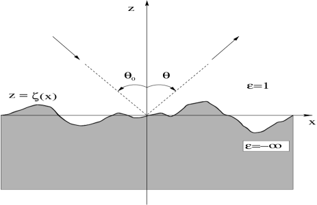
FIG. 1.: The scattering geometry considered in this paper.

for all positive real numbers $\mu$. Here $H$ is the roughness exponent, also known as the Hurst exponent, and it characterizes this invariance. This exponent is usually found in the range from zero to one. A statistical translation of the previous statement is that the probability $p(\Delta\zeta;\Delta x)$ of having a height difference in the range $[\Delta\zeta,\Delta\zeta+d\Delta\zeta]$ over the (lateral) distance $\Delta x$ is such that:

$$p\left(\Delta\zeta;\Delta x\right)d\Delta\zeta=p\left(\mu^{H}\Delta\zeta;\mu\Delta x\right)d\mu^{H}\Delta\zeta.$$ (4)

Simple algebra based on the scaling relation (II) gives that the standard deviation of the height differences $\zeta(x+\Delta x)-\zeta(x)$ measured over a window of size $\Delta x$ can be written as

$$\sigma(\Delta x) = \ell^{1-H}\Delta x^{H},$$ (6)

and the (mean) slope of the surface as

$$s(\Delta x) = \left(\frac{\ell}{\Delta x}\right)^{1-H}.$$ (7)

In these equations $\ell$ denotes a length scale known as the topothesy. It is defined as $\sigma(\ell)=\ell$ (or $s(\ell)=1$).

Alternatively, Eq. (6) can be written in the form

$$\sigma\left(\Delta x\right)=\sigma(\lambda)\left(\frac{\Delta x}{\lambda}\right)^{H}=\lambda s(\lambda)\left(\frac{\Delta x}{\lambda}\right)^{H}\;,$$ (8)

where we use the wavelength $\lambda$ of the scattering problem as a normalization length. Here $\sigma(\lambda)$ and $s(\lambda)$ are respectively the typical height difference and slope over one wavelength as defined by Eqs. (II). Note that we could have used any length scale for the normalization, like for instance the topothesy. However, the choice made here was dictated by the physical problem studied. Using similar scaling arguments one can show that the power density function of the height profile ${\cal P}(k)$ depends on the wave number $k$ as a power law:

$${\cal P}(k)=\left|\int_{-\infty}^{\infty}\zeta(x)\exp(ikx)dx\right|^{2}\propto k^{-1-2H}.$$ (9)

In the case of a Gaussian height distribution, the probability $p(\Delta\zeta;\Delta x)$ reads:

$$p(\Delta\zeta;\Delta x)=\frac{\lambda^{H-1}}{\sqrt{2\pi}s(\lambda)\Delta x^{H}}\exp\left[-\frac{1}{2}\left(\frac{\lambda^{H-1}\Delta\zeta}{s(\lambda)\Delta x^{H}}\right)^{2}\right].$$ (10)

The self-affine profile is thus fully characterized by the roughness exponent $H$, the slope $s(\lambda)$ (which is nothing but an amplitude parameter) and the bounds of the self-affine regime $\xi_{-}$ and $\xi_{+}$.

Numerous methods have been developed to estimate these parameters (see for example Ref. [34]), most of them use the expected power law variation of a roughness estimator computed over spatial ranges of varying size. This roughness estimator can be a height standard deviation, the difference between the maximum and the minimum height, etc. It is also classical to use directly the power density function of the profile. More recently the wavelet analysis has beeen shown to offer a very efficient method to compute the roughness exponent of self-affine surfaces [35].

III Scattering Theory

In the following we consider the scattering of $s$-polarized electromagnetic waves from a one-dimensional, random, Gaussian self-affine surface $z=\zeta(x)$. It will be assumed that the lower limit of the self-affine regime $\xi_{-}$ is smaller than the wavelength, $\lambda$, of the incident wave. For the present scattering system, where the roughness is one-dimensional, the complexity of the problem is reduced significantly. The reason being that there is no depolarization and therefore the original three-dimensional vector scattering problem reduces to a two-dimensional scalar problem for the single non-vanishing 2nd component for the electric field, $\Phi(x,z|\omega)=E_{y}(x,z|\omega)$, which should satisfy the (scalar) Helmholtz equation

$$\left(\partial^{2}_{x}+\partial^{2}_{z}+\frac{\omega^{2}}{c^{2}}\right)\Phi(x,z|\omega) = 0,$$ (11)

with vanishing boundary condition on the randomly rough surface $z=\zeta(x)$, and outgoing wave condition at infinity. In the far field region, above the surface, the field can be represented as the sum of an incident wave and scattered waves:

$$\Phi(x,z|\omega) = \Phi_{0}(x,z|\omega)+\int^{\infty}_{-\infty}\;\frac{dq}{2\pi}R(q|k)\;e^{iqx+i\alpha_{0}(q,\omega)z},$$ (12)

where the plane incident wave is given by:

$$\Phi_{0}(x,z|\omega) = \exp\left\{ikx-i\alpha_{0}(k,\omega)z\right\}$$ (13)

and $R(q|k)$ is the scattering amplitude. In the above expressions, we have defined

$$\alpha_{0}(q,\omega) = \sqrt{\left(\frac{\omega}{c}\right)^{2}-q^{2}},\quad{\Re}\alpha_{0}(q,\omega)>0,{\Im}\alpha_{0}(q,\omega)>0.$$ (14)

Furthermore, the (longitudinal) momentum variables $q$ and $k$ are in the radiative region related to respectively the scattering and incident angle by

$$k = \frac{\omega}{c}\sin\theta_{0},$$ (16)

$$q = \frac{\omega}{c}\sin\theta,$$ (17)

so that the $z$-components of the incident and scattering wavenumbers become

$$\alpha_{0}(k,\omega) = \frac{\omega}{c}\cos\theta_{0},$$ (18)

$$\alpha_{0}(q,\omega) = \frac{\omega}{c}\cos\theta.$$ (19)

The mean differential reflection coefficient (DRC), also known as the mean scattering cross section, is an experimentally accessible quantity. It is defined as the fraction of the total, time-averaged, incident energy flux scattered into the angular interval $(\theta,\theta+d\theta)$. It can be shown to be related to the scattering amplitude by the following expression [36]:

$$\left<\frac{\partial R_{s}}{\partial\theta}\right> = \frac{1}{L}\;\frac{\omega}{2\pi c}\;\frac{\cos^{2}\theta}{\cos\theta_{0}}\left<\left|R(q|k)\right|^{2}\right>.$$ (20)

Here $L$ denotes the length covered by the self-affine profile as measured along the $x$-direction, and the other quantities have been defined earlier. The angle brackets denote an average over an ensemble of realizations of the rough surface profiles. Moreover, the momentum variables appearing in Eq. (20) are understood to be related to the angles $\theta_{0}$ and $\theta$ according to Eqs. (III).

We now impose the Kirchhoff approximation which consists of locally replacing the surface by its tangential plane at each point, and thereafter using the (local) Fresnel reflection coefficient for the local angle of incidence to obtain the scattered field. Notice that dealing with a surface whose scaling invariance range is bounded by a lower cut-off $\xi_{-}$ does ensure that the tangential plane is well defined at every point. Within the Kirchhoff approximation the scattering amplitude can be expressed as [36]:

$$R(q|k) = \frac{-i}{2\alpha_{0}(q,\omega)}\int^{L/2}_{-L/2}dx\;e^{-iqx-i\alpha_{0}(q,\omega)\zeta(x)}{\cal N}_{0}(x|\omega),$$ (22)

where ${\cal N}_{0}(x|\omega)$ is a source function defined by

$${\cal N}_{0}(x|\omega) = 2\,\partial_{n}\!\!\left.\Phi_{0}(x,z|\omega)\right|_{z=\zeta(x)}.$$ (23)

Here $\partial_{n}$ denotes the (unnormalized) normal derivative defined as $\partial_{n}=-\zeta^{\prime}(x)\partial_{x}+\partial_{z}$.

By substituting the expression for the scattering amplitude , Eq. (22), into Eq. (20), one obtains an expression for the mean differential reflection coefficient in terms of the source function ${\cal N}_{0}(x|\omega)$; the normal derivative of the total field evaluated on the rough surface. After some straightforward algebra where one takes advantage of the fact that the self-affine surface profile function $\zeta(x)$ has stationary increments, one obtains the following form for the mean differential reflection coefficient

$$\left<\frac{\partial R_{s}}{\partial\theta}\right> = \displaystyle{\frac{\omega}{2\pi c}\frac{1}{\cos\theta_{0}}\left(\frac{\cos\left[(\theta+\theta_{0})/2\right]}{\cos\left[(\theta-\theta_{0})/2\right]}\right)^{2}}\int^{L/2}_{-L/2}dv\;\exp\left\{i\frac{\omega}{c}(\sin\theta-\sin\theta_{0})v\right\}\Omega(v),$$ (25)

where

$$\Omega(v) = \left<\exp\left\{-i\frac{\omega}{c}[\cos\theta+\cos\theta_{0}]\,\Delta\zeta(v)\right\}\right>,$$ (26)

with $\Delta\zeta(v)=\zeta(x)-\zeta(x+v)$. Note that the statistical properties of the profile function, $\zeta(x)$, enters Eqs. (III) only through $\Omega(v)$. With the height distribution $p(\delta\zeta;\delta x)$ introduced earlier, Eq. (10), one may now analytically calculate the ensemble average contained in $\Omega(v)$. For a Gaussian self-affine surface one gets

$$\Omega(v) = \int^{\infty}_{-\infty}dz\;\exp\left\{-i\frac{\omega}{c}\left(\cos\theta+\cos\theta_{0}\right)z\right\}p(z;v)$$ (27)

$$= \exp\left\{-\left(\frac{\omega}{c}\frac{\cos\theta+\cos\theta_{0}}{\sqrt{2}}s(\lambda)\lambda^{1-H}v^{H}\right)^{2}\right\}.$$ (28)

By in Eq. (III) making the change of variable

$$u = v\left[\frac{\omega}{c}\frac{\cos\theta+\cos\theta_{0}}{\sqrt{2}}s(\lambda)\lambda^{1-H}\right]^{1/H}\;,$$ (29)

and letting the length of the profile extend to infinity, $L\rightarrow\infty$, one finally obtains the following expression for the mean differential reflection coefficient:

$$\left<\frac{\partial R_{s}}{\partial\theta}\right> = \frac{s(\lambda)^{-\frac{1}{H}}a^{-(\frac{1}{H}-1)}}{\sqrt{2}\,\cos\theta_{0}}\frac{\cos\frac{\theta+\theta_{0}}{2}}{\cos^{3}\frac{\theta-\theta_{0}}{2}}{\cal L}_{2H}\left(\frac{\sqrt{2}\tan\frac{\theta-\theta_{0}}{2}}{a^{\frac{1}{H}-1}s(\lambda)^{\frac{1}{H}}}\right),$$ (31)

where

$$a = 2\pi\sqrt{2}\cos\frac{\theta+\theta_{0}}{2}\cos\frac{\theta-\theta_{0}}{2},$$ (32)

and ($0<\alpha\leq 2$)

$${\cal L}_{\alpha}(x) = \frac{1}{2\pi}\int^{\infty}_{-\infty}dk\;e^{ikx}e^{-\left|k\right|^{\alpha}}.$$ (33)

The quantity ${\cal L}_{\alpha}(x)$ is known as the centered symmetric Lévy stable distribution of index (or order) $\alpha$ [37]. This distribution can only be expressed in closed form for some particular values of $\alpha=$; $\alpha=1$ and $\alpha=2$correspond to the Cauchy-Lorentzian and Gaussian distributions respectively, ${\cal L}_{1/2}$ and ${\cal L}_{1/3}$ can be expressed from special functions. When the $\alpha$-index in the Lévy distribution ${\cal L}_{\alpha}(x)$ is lowered from its upper value $\alpha=2$ (Gaussian distribution), the resulting distribution develops a sharper peak at $x=0$ while at the same time its tails become fatter. It is interesting to note from Eqs. (III) that the wavelength, $\lambda=2\pi c/\omega$, only comes into play through the slope $s(\lambda)$. The behavior of the scattered intensity is thus entirely determined by this typical slope $s(\lambda)$ and the roughness exponent $H$.

FIG. 2.: The mean differential reflection coefficient, $\left<\partial R_{s}/\partial\theta\right>$, vs. scattering angle, $\theta$, for a perfectly conducting self-affine surface. The plotted curves are the prediction of Eqs. (III). The Hurst exponent in all cases are $H=0.7$ and topothesies $\ell$ are ranging from $\ell=10^{-2}\lambda$ ($S(\lambda=0.016$) down to $10^{-6}\lambda$ ($s(\lambda)=0.25$) as indicated in the figures. The angles of incidence were (a) $\theta_{0}=0^{\circ}$ and (b) $\theta_{0}=0^{\circ}$.

In Figs. 2 we show the mean differential reflection coefficient as obtained from Eqs. (III) for Hurst exponent $H=0.7$ and different values of the slope $s(\lambda)$ ranging from $0.016$ to $0.25$. The angles of incidence were $\theta_{0}=0^{\circ}$ (Fig. 2a) and $50^{\circ}$ (Fig. 2b). It is observed from these figures that as the amplitude parameter $s(\lambda)$ is decreased, while keeping the other parameters fixed, the portion of the scattered intensity scattered diffusely is reduced, while the power-law behavior found for the non-specular directions survives independently (within single scattering) of the amount of light scattered specularly. Furthermore, as the Hurst exponent is decreased (results not shown), and thereby making the topography rougher at small scale, the mean DRC gets a larger contribution from diffusely scattered light. This is a direct consequence of the properties of the Lévy distribution mentioned above.

In order to discuss the features of the mean DRC which can be seen in Figs. 2 we will now proceed by discussing the behavior of the specular and diffuse contribution to $\left<\partial R_{s}/\partial\theta\right>$, i.e. close and far away from the scattering angle $\theta=\theta_{0}$ respectively.

A The specular contribution

We start by considering the specular contribution to the mean differential reflection coefficient. This is done by taking advantage of the asymptotic expansion of the Lévy distribution around zero [38]

$${\cal L}_{\alpha}(x) = \frac{1}{\pi\alpha}\Gamma\left(\frac{1}{\alpha}\right)\left[1-\frac{\Gamma\left(\frac{3}{\alpha}\right)}{2\Gamma\left(\frac{1}{\alpha}\right)}x^{2}\right]+{\cal O}(x^{4}).$$ (34)

By substituting this expression into Eqs. (III) one finds that the mean DRC around the speular direction $\theta=\theta_{0}$ should behave as follows ($\delta\theta\ll 1$)

$$\left.\left<\frac{\partial R_{s}}{\partial\theta}\right>\right|_{\theta=\theta_{0}+\delta\theta} = \frac{\Gamma\left(\frac{1}{2H}\right)}{2\sqrt{2}\pi H\left(2\sqrt{2}\pi\cos\theta_{0}\right)^{\frac{1}{H}-1}s(\lambda)^{1/H}}$$ (36)

$$\quad\times\left[1+\delta\theta\frac{1-2H}{2H}\tan\theta_{0}+\frac{(\delta\theta)^{2}}{4}\left(1+\frac{1+H}{2H^{2}}\tan^{2}\theta_{0}-\frac{\Gamma(\frac{3}{2H})}{\Gamma(\frac{1}{2H})\left(2\sqrt{2}\pi\cos\theta_{0}\right)^{\frac{2}{H}-2}s(\lambda)^{2/H}}\right)\right].$$

From this expression it follows that the amplitude of the specular peak should scale as

$$\left.\left<\frac{\partial R_{s}}{\partial\theta}\right>\right|_{\theta=\theta_{0}}\simeq\frac{\Gamma(\frac{1}{2H})}{2\sqrt{2}\pi H\left(2\sqrt{2}\pi\cos\theta_{0}\right)^{\frac{1}{H}-1}s(\lambda)^{1/H}},$$ (37)

and that the peaks half width at half maximum, $w$, should be given by

FIG. 3.: The full single scattering solution (solid line), Eqs. (III), for the mean differential reflection coefficient vs. scattering angle $\theta$ for a perfectly conducting self-affine surface compared to its specular (dotted line) and diffuse expansions (dashed line) as given by respectively Eqs. (36) and (41). The surface parameters used were $H=0.7$ and $\ell=10^{-4}\lambda$ ($s(\lambda)=0.063$), and the light was incident normally onto the rough surface.

$$w\left(H,s(\lambda),\theta_{0}\right) \simeq 2\sqrt{\frac{\Gamma(\frac{1}{2H})}{\Gamma(\frac{3}{2H})}}\left(2\sqrt{2}\pi\cos\theta_{0}\right)^{\frac{1}{H}-1}s(\lambda)^{1/H}\;.$$ (38)

It is worth noting that in the above expression the width of the specular peak depends on the wavelength $\lambda$ via the typical slope over one wavelength $s(\lambda)$. In case of Gaussian correlations, there would have been no dependence on the wavelength, the peak width $w$ being simply proportional to the ratio $\sigma/\tau$, RMS roughness over correlation length.

In order to test the quality of the specular expansion, Eq. (36), we show in Fig. 3 a comparison of this expression with the full single scattering solution obtained from Eqs. (III) for a surface of roughness exponent $H=0.7$ and of slope over the wavelength $s(\lambda)=0.063$ ($\ell=10^{-4}\lambda$) in case of normal incidence. The amplitude of the specular peak is seen to be nicely reproduced, but this expansion is only valid within a rather small angular interval around the specular direction $\theta=\theta_{0}$.

It is interesting to notice that in the case of a non-zero angle of incidence, $\theta_{0}\neq 0^{\circ}$, the specular peak is slightly shifted away from its expected position $\theta=\theta_{0}$ due to the presence of a non-vanishing term in Eq. (36) linear in $\delta\theta$. In this case the apparent specular peak is located at $\theta=\theta_{0}+\Delta\theta_{0}$, where $\Delta\theta_{0}$ ($\Delta\theta_{0}\sim w^{2}\ll w$) scales as

$$\Delta\theta_{0}\simeq\frac{2H-1}{H}\frac{\Gamma(\frac{1}{2H})}{\Gamma(\frac{3}{2H})}\tan\theta_{0}\left(2\sqrt{2}\pi\cos\theta_{0}\right)^{\frac{2}{H}-2}s(\lambda)^{2/H}\;=\;\frac{2H-1}{4H}\tan\theta_{0}w^{2}(H,s(\lambda),\theta_{0})$$ (39)

Such a shift has not, to our knowledge, been reported earlier for non self-affine (or non fractal) surfaces. Hence, due to the self-affinity of the random surface, we predict a shift, $\Delta\theta_{0}$, in the specular direction as compared to its expected position at $\theta=\theta_{0}$. Notice that this shift vanishes for a Brownian random surface ($H=1/2$). Moreover, for a persistent surfaces profile function ($H>1/2$) the shift is positive while it becomes negative for anti-persistent profile ($H<1/2$). Unfortunately the specular shift $\Delta\theta_{0}$ is probably too small to be observable experimentally for realizable self-affine parameters.

B The diffuse component

We now focus on the diffuse component to the mean differential reflection coefficient, i.e. the region where $\theta$ is far away from $\theta=\theta_{0}$. Now, using the expansion of the Lévy distribution at infinity (the Wintner development) [38]

$${\cal L}_{\alpha}(x) = \frac{\Gamma(1+\alpha)}{\pi|x|^{1+\alpha}}\sin\left(\frac{\alpha\pi}{2}\right)+{\cal O}\left(\frac{1}{|x|^{1+2\alpha}}\right),$$ (40)

we get the following expression for the diffuse component of the mean DRC ($\theta\neq\theta_{0}$)

$$\left<\frac{\partial R_{s}}{\partial\theta}\right>\simeq\frac{\Gamma(1+2H)\sin(\pi H)}{\left(4\pi\right)^{2H-1}}\frac{s(\lambda)^{2}}{\cos\theta_{0}}\frac{\left|\cos\frac{\theta+\theta_{0}}{2}\right|^{3-2H}}{\left|\sin\frac{\theta-\theta_{0}}{2}\right|^{1+2H}}\;.$$ (41)

In Fig. 3 the above expression is compared to the prediction of Eqs. (III). We observe an excellent agreement for angular distances larger than ten degrees. Moreover, it should be noticed from Eq. (41) that the mean DRC is predicted to decay as a power-law of exponent $-1-2H$ as we move away from the specular direction. For smooth surfaces (corresponding to small values of $s(\lambda)$) this behavior results directly from a perturbation approach where the scattered intensity derived directly from the power density function of the surface. As shown above, in the case of self-affine surfaces the latter is a power law of exponent $-1-2H$. Our results extend then the validity of this power law regime to steeper surfaces.

IV Scaling analysis

It is interesting that most of the non-trivial scaling results derived above can be retrieved via simple dimensional arguments. Let us examine the intensity scattered in direction $\theta$; in a naive Huyghens framework two different effects will compete to destroy the coherence of two source points on the surface i) the angular difference separating $\theta$ from the specular direction and ii) the roughness. Considering two points separated by a horizontal distance $\Delta x$ and a vertical distance $\Delta z$, we can define the retardation due to these two effects:

$$\Delta c_{ang}=(\sin\theta-\sin\theta_{0})\Delta x\;,\quad\Delta c_{rough}=(\cos\theta+\cos\theta_{0})\Delta z\;.$$

This allows us to define two characteristic (horizontal) lengths $\delta_{ang}$ and $\delta_{rough}$ of the scattering system corresponding to the distances between two points of the surface such that $\Delta c_{ang}$ and $\Delta c_{rough}$ are equal to the wavelength $\lambda$. Taking into account the self-affine character of the surface, we get:

$$\delta_{ang}=\frac{\lambda}{\sin\theta-\sin\theta_{0}}\;,\quad\delta_{rough}=\frac{\lambda}{(\cos\theta+\cos\theta_{0})^{1/H}}s(\lambda)^{-1/H}\;.$$

The coherence length on the surface depends on the relative magnitude of these two characteristic lengths. For scattering angles close to the specular direction, we have $\delta_{rough}\ll\delta_{ang}$ and for large scattering angles $\delta_{ang}\leq\delta_{rough}$ and the diffuse tail is controlled by the angular distance to the specular direction. In general we can evaluate the competition of these two effects and their consequences on the scattering cross-section by the simple ratio of the two characteristic lengths:

$$\chi=\frac{\delta_{rough}}{\delta_{ang}}=\frac{\sin\theta-\sin\theta_{0}}{(\cos\theta+\cos\theta_{0})^{1/H}}s(\lambda)^{-1/H}\;.$$

We can then describe our scattering system with this unique variable $\chi$ which takes into account the incidence and scattering directions, the roughness parameters of the surface and the wavelength. A direct application is the determination of the angular width $w$ of the specular peak. The transition between the specular peak and the diffuse tail is simply defined by $\chi=1$ which leads to:

$$w\simeq[2s(\lambda)]^{1/H}(\cos\theta_{0})^{1/H-1}$$

which is identical to the exact result (38) apart from a numerical constant. Assuming that most of the intensity is scattered within the specular peak, we obtain via the energy conservation

$$\left.\left<\frac{\partial R_{s}}{\partial\theta}\right>\right|_{\theta=\theta_{0}}\simeq\frac{1}{w}\simeq[2s(\lambda)]^{-1/H}(\cos\theta_{0})^{1-1/H}$$

Forgetting the numerical constants, we can thus rewrite the scattering cross-section as

$$\left<\frac{\partial R_{s}}{\partial\theta}\right>=\frac{(\cos\theta_{0})^{1-1/H}}{s(\lambda)^{1/H}}\Psi(\chi)$$

When approaching the specular direction we note that $\delta_{ang}$ diverges whereas $\delta_{rough}$ saturates at a finite value independent on the angular direction. In this specular direction, the scattering process is thus controlled by only the latter length and does not depend on the ratio $\chi=\delta_{rough}/\delta_{ang}$. This imposes:

$$\Psi(\chi)\simeq 1,\qquad(\chi\ll 1).$$

The argument $\chi$ being inversely proportional to the quantity $s(\lambda)^{1/H}$ which is nothing but a roughness amplitude parameter, the behavior of $\Psi$ for large arguments can be found by matching our expresion with the limit of very smooth surfaces. In this limit a simple perturbation approach leads to:

$$\left<\frac{\partial R_{s}}{\partial\theta}\right>\propto{\cal P}\left[\frac{2\pi}{\lambda}(\sin\theta-\sin\theta_{0})\right],$$

where ${\cal P}$ is the power density function of the height profile. In the case of a self-affine profile of roughness exponent $H$, we have ${\cal P}(k)\propto k^{-1-2H}$. One can check that this can only be consistent with the same power law behavior for $\Psi$:

$$\Psi(\chi)\propto\chi^{-1-2H},\qquad(\chi\gg 1).$$

V Numerical simulation results and discussion

The results obtained in the previous sections were all based on the Kirchhoff approximation, and will therefore only be accurate in cases where single scattering is dominating. In this section, however, we will therefore no longer restrict ourselves to single scattering, but instead include any higher order scattering process. This is accomplished by a rigorous numerical simulations approach which will be described below. This approach will also serve as an independent check of the correctness of the analytic results (III), and the results that can be derived thereof. Furthermore, it will also provide valuable insight into which part of parameter space is dominated by single scattering processes, and thus where formulae (III) can be used with confidence.

The rigorous numerical simulation calculations for the mean differential reflection coefficient were performed for a plane incident $s$-polarized wave scattered from a perfectly conducting rough self-affine surface. Such simulations were done by the now quite standard extinction theorem technique [36]. This technique amounts to using Green’s second integral identity to write down the following inhomogeneous Fredholm equation of the second kind for the source function ${\cal N}(x|\omega)$ (see Refs. [39, 40]):

$${\cal N}(x|\omega)=2{\cal N}_{0}(x|\omega)-2\,{\cal P}\!\!\int dx^{\prime}\;\left.\partial_{n}G_{0}(x,z|x^{\prime},z^{\prime})\right|_{z^{\prime}=\zeta(x^{\prime})}{\cal N}(x^{\prime}|\omega).$$ (43)

In this equation

$${\cal N}(x|\omega) = \left.\partial_{n}\Phi(x,z|\omega)\right|_{z=\zeta(x)},$$ (44)

where $\partial_{n}=-\zeta^{\prime}(x)\partial_{x}+\partial_{z}$ is the (unnormalized) normal derivative of the total electric field $\Phi=E_{y}$ evaluated on the randomly rough self-affine surface, ${\cal N}_{0}(x|\omega)$ has been defined earlier as the normal derivative of the incident field, and ${\cal P}$ is used to denote the principle part of the integral. Moreover, $G_{0}(x,z|x^{\prime},z^{\prime})$ is the (two-dimensional) free space Greens function defined by

$$G_{0}(x,z|x^{\prime},z^{\prime}) = i\pi H^{(1)}_{0}\left(\frac{\omega}{c}\left|{\bf r}-{\bf r}^{\prime}\right|\right),$$ (45)

where ${\bf r}=(x,z)$, ${\bf r^{\prime}}=(x^{\prime},z^{\prime})$ and $H^{(1)}_{0}(x)$ denotes the 0 th order Hankel function of the first kind [41]. By taking advantage of Eq. (22) which relates the scattering amplitude to the normal derivative of the total field on the random surface, the scattering amplitude can easily be calculated, and from there the mean differential reflection coefficient. It should be noticed that the Kirchhoff approximation used in the previous section to obtain the analytical results (III), is obtained from by Eq. (43) by neglecting the last (integral) term that represents multiple scattering. By using a numerical quadrature scheme [42], the integral equation, Eq. (43), can be solved for any given realization of the surface profile $\zeta(x)$. From the knowledge of ${\cal N}(x|\omega)$ one might then easily calculate the mean DRC.

Randomly rough Gaussian self-affine surfaces of given Hurst exponent were generated by the Fourier filtering method [43] (see Eq. (9)), i.e. in Fourier space to filter complex Gaussian random uncorrelated numbers by a decaying power-law filter of exponent $-H-1/2$ and thereafter transforming this sequence into real space. The topothesis (or slope) of the surfaces were then adjusted to the desired values, $\ell$, by taking advantage of Eq. (II). This is done by first calculating the topothesy, $\ell_{0}$, of the original surface over its total length and thereafter rescaling the profile by $(\ell_{0}/\ell)^{1-H}$, where $\ell$ is the desired topothesy. In order to having enough statistical information to be able to calculate a well-defined topothesy $\ell_{0}$, we in fact used a window size slightly smaller than the total length of the surface.

FIG. 4.: A comparison plotted in (a) linear- and (b) linear-log scale, of the mean differential reflection coefficient $\left<\partial R_{s}/\partial\theta\right>$ vs. scattering angle $\theta$ for a perfectly conducting self-affine surface obtained by a rigorous numerical simulations approach (solid lines), and therefore including all possible multiple-scattering processes, and the single-scattering results obtained from Eqs. (III) (dashed lines). The surface parameters were $H=0.7$ and $\ell=10^{-4}\lambda$ ($s(\lambda)=0.063$) with $\lambda=612.7{\rm nm}$. The angles of incidence for the light were $0^{\circ}$ and $50^{\circ}$ as indicated in the figure.

By the methods just described, we have performed rigorous numerical simulations for the mean differential reflection coefficient, $\left<\partial R_{s}/\partial\theta\right>$, in the case of a $s$-polarized plane incident wave of wavelength $\lambda=2\pi c/\omega=612.7~{}{\rm nm}$ that is scattered from a perfectly conducting self-affine surface characterized by the Hurst exponent, $H$, and the topothesy $\ell$. For all simulation results shown, the length of the surface was $L=100\lambda$, and the spatial discretization length was $\Delta x\simeq\lambda/10$. All simulation results presented were averaged over $N_{\zeta}=1000$ surface realizations (or more). Furthermore, in order to check the quality of the numerical simulations, both reciprocity and unitarity were checked for all simulation results. It was found for all cases considered that the reciprocity was satisfied within the noise level of the calculations, while the unitarity was fulfilled within an error of a fraction of a percent.

In Figs. 4 the mean differential reflection coefficients for a surfaces characterized by the parameters $H=0.7$ and $\ell=10^{-4}\lambda$ ($s(\lambda)=0.063$) are presented. The angles of incidence of the light were $\theta_{0}=0^{\circ}$ and $50^{\circ}$ as indicated in the figures. The solid lines represents the numerical (multiple-scattering) simulation results while the dashed lines are the (single-scattering) prediction of Eqs. (III). As can be seen from Fig. 4a the correspondence is quite good between the analytic results and those obtained from the numerical simulations. To allow a better comparison for large scattering angles we present in Fig. 4b the results of Fig. 4a, but now in a linear-log scale. From this figure it is apparent that for the largest scattering angles there are some disagreements between the analytic and numerical results. The analytic results tend to overestimate the mean DRC in these regions. This discrepancy stems from the fact that multiple scattering is not included in the analytical results. Part of the light that according to single scattering would have been scattered into large scattering angles are now due to multiple scattering processes, scattered back into smaller

FIG. 5.: The same as Figs. 2 (single scattering results), but now using a rigorous numerical simulation approach (see text for details) that incorporate all higher order scattering processes.

FIG. 6.: The specular peak amplitude, $\left.\left<\partial R_{s}/\partial\theta\right>\right|_{\theta=\theta_{0}}$, and its half width at half maximum, $w(H,\ell/\lambda,\theta_{0})$ as a function of the topothesy $\ell$. The angle of incidence was in both cases $\theta_{0}=0^{\circ}$. The solid lines are analytical results obtained from Eqs. (37) and (38) respectively, while the circles (amplitudes) and the squares (widths) are obtained from the numerical simulations results shown in Fig. 5a.

angles. This results in smaller values for $\left<\partial R_{s}/\partial\theta\right>$ for the largest scattering angles. Since the unitarity condition, $\int^{\pi/2}_{-\pi/2}\left<\partial R_{s}/\partial\theta\right>\,d\theta=1$, is satisfied for a perfectly reflecting surface, this large angle reduction of the mean DRC has to be compensated by an increase for other scattering angles. In the case of normal incidence ($\theta_{0}=0^{\circ}$) say, this increase can be seen in the region around $|\theta|\sim 25^{\circ}$ where the numerical simulation results are bigger then the corresponding single-scattering analytical results. The same behavior can be observed for an angle of incidence of $50^{\circ}$.

We give in Figs. 5 the numerical simulation results for five different values of the topothesy ranging from $\ell=10^{-6}\lambda$ ($S(\lambda=0.016$) up to $10^{-2}\lambda$ ($s(\lambda)=0.25$). These multiple-scattering results should be compared to the results of Figs. 2 which show the corresponding curves obtained from Eqs. (III). The roughness exponent used in the simulations leading to the results of Figs. 5 was in all cases $H=0.7$, while for the angles of incidence we used $\theta_{0}=0^{\circ}$ (Fig. 5a) and $\theta_{0}=50^{\circ}$ (Fig. 5b). The height standard deviation as measured over the whole length of the surface, $L=100\lambda$, was according to Eq. (II) ranging from $\sigma(L)=0.4\lambda$ for the smallest topothesy up to as large as $6.3\lambda$ for the largest. The fact that we did not really use the total length, $L$, during the surface generation when adjusting the topothesy, but instead a slightly smaller fraction of this length, did not seem to affect the height standard deviation to a large degree. In fact it was found numerically that the RMS-heights of the generated surfaces were only a few percent lower then the one obtained from using Eq. (II) and we will therefore in the following use this equation in estimating the RMS-height of the surfaces. According to optical criterion these surface roughness correspond to rather rough surfaces. In particular one observes from Fig. 5 that in the case of $\ell=10^{-2}\lambda$ a specular peak is hard to define at all in the mean DRC spectra. This is a clear indication of a highly rough surface and thus a very severe test of our theory.

To further compare the analytic results derived earlier with those obtained from the numerical simulation approach, we in Fig. 6 have plotted the amplitude of the specular peaks (circles) $\left.\left<\partial R_{s}/\partial\theta\right>\right|_{\theta=\theta_{0}}$, and their width (squares) $w(H,\ell/\lambda,\theta_{0})$, as obtained from the numerical simulation results shown in Figs. 5. The solid lines of this figure are the analytic predictions for these quantities as given respectively by Eqs. (37) and (38). As can be seen from this figure, the analytic predictions are in excellent agreement with their numerical simulation counterparts. In particular this confirms the decaying and increasing power-laws in topothesy of exponent $1/H-1$ for these two quantities respectively.

From Eqs. (III) we observe that if we replot the mean DRC times the inverse of the prefactor of the Lévy distribution, vs. its argument, all mean DRC-curves corresponding to the same Hurst exponent should (within single-scattering) collapse onto one and the same master curve. This master curve should be the Lévy distribution, ${\cal L}_{2H}(x)$, of order $2H$. Notice that this data-collapse should hold true for arbitrary values for the angle of incidence and topothesy. The failure of such a data-collapse (onto ${\cal L}_{2H}$) indicates essential contributions from multiple-scattering effects. The range of scattering angles where such processes are important can therefore be read off from such a plot. Furthermore, since the tails of the Lévy distribution ${\cal L}_{2H}(x)$ drops off like $x^{-2H-1}$ (cf. Eq. (40)) such rescaled mean DRC plots can be used to measure the Hurst exponent of the underlying self-affine surfaces for which the light scattering data have been obtained. In order to check these predictions for our numerical simulations results, we present in Fig. 7 such a rescaling of the data originally presented in Fig. 5b. Only data lying to the left of the specular peak have been included, i.e. only data for scattering angles $\theta<\theta_{0}=50^{\circ}$. As can be seen from this figure the various scattering curves nicely fall onto the master-curve (solid line) in regions where single-scattering is dominating. When

FIG. 7.: Rescaled version of the rigorous numerical simulation results shown in Fig. 5b. Only the data corresponding to $\theta<50^{\circ}$ are included. In the rescaled coordinates all data (symbols) should within the single scattering approximation collapse onto a Lévy distribution of order $2H$ (solid line).

multiple scattering processes start giving a considerable contribution the scattering curves start to deviate from this master-curve. This observation could be used in practical applications to determine for what regions the scattering is dominated by single scattering processes. For the lowest topothesy considered here, $\ell=10^{-6}\lambda$, a power-law extends nicely over large regions of scattering angels — a signature of the diffuse scattering from self-affine surfaces. According to Eq. (41) the exponent of this power-law should be $-1-2H$. A regression fit to the scattering curve corresponding to the topothesy $\ell=10^{-6}\lambda$ gives $H=0.73\pm 0.02$, where the error indicated is a pure regression error. The real error is of course larger. With the knowledge of the Hurst exponent obtained from the decay of the diffuse tail of the mean DRC, we might now, based on the amplitude of the specular peak, obtain an estimate for the topothesy of the surface. From the numerical simulation result we have that $\left.\left<\partial R_{s}/\partial\theta\right>\right|_{\theta=\theta_{0}}\simeq 17.9$ which together with Eq. (37) gives $\ell=0.97\cdot 10^{-6}\,\lambda$, where we have used the value found above for the Hurst exponent. These two results fit quite nicely with the values $H=0.7$ and $\ell=10^{-6}\lambda$ used in the numerical generation of the underlying self-affine surfaces.

It should be noticed that for the numerical results presented in this paper, we have not considered topothesies smaller then $\ell=10^{-6}\lambda$. However, since lowering the topothesy will, as also indicated by our numerical results, favor single-scattering processes over those obtained from multiple scattering, the analytic results (III) will trivially be valid for low values of the topothesy. This has also been checked explicitly by numerical simulations (results not shown).

So far in this paper we have assumed that the metal was a perfect conductor. Obviously this is an idealization, and even the best conductors known today are not perfect conductors at optical wavelengths. By relaxing the assumption of the metal being perfectly conducting to instead being a good conductor, i.e. a real metal, we are no longer in position to obtain a closed form solution of the scattering problem, the reason being that the boundary conditions are no longer local quantities. In this latter case we therefore have to resort to numerical calculations in any case. In order to see how well our analytic results (III) describe the scattering from real metals (in contrast to perfect conductors) we in Fig. 8 give the mean DRC, as obtained from numerical simulations [36], for a self-affine silver surface of Hurst exponent $H=0.7$ and topothesy $\ell=10^{-4}\lambda$. We recall that this choice for the topothesy corresponds to a rather rough surface where the RMS-height measured over the whole length of the surface is $\sigma(L)\sim 1.45\lambda$. Furthermore, the angles of incidence were $\theta=0^{\circ}$ and $50^{\circ}$ and the wavelength of the incident light was $\lambda=612.7~{}{\rm nm}$. At this wavelength the dielectric constant of silver is $\varepsilon(\omega)=-17.2+0.50i$ [44]. The long dashed lines of Fig. 8 represent the predictions from Eqs. (III), and as can be seen from this figure, the correspondence is rather good. It is interesting to see that the agreement between the analytical and numerical results is of the same quality as the one found for the perfect conductor (see Fig. 4b). This indicates that the analytic results given by Eqs. (III) are rather robust and tend to also describe well the scattering from a good, but not necessary perfect, reflector. Simulations equivalent to those reported for silver have also been performed for aluminum (results not shown) which has a dielectric function that is more then three times higher at the wavelength ($\lambda=612.7{\rm nm}$) used here. The conclusions found above for silver also hold true for aluminum. We find it interesting to note that such self-affine aluminum surfaces were recently reported to be seen for cold rolled aluminum [17]. The Hurst exponents were measured to be $H=0.93\pm 0.03$ and $H=0.50\pm 0.05$ for the transverse

FIG. 8.: The same as Fig. 4b, but now using a real metal (silver) instead of a perfect conductor. The value of the dielectric constant of silver at the wavelength of the incident light ($\lambda=612.7{\rm nm}$) was $\varepsilon(\omega)=-17.2+0.50i$.

and longitudinal direction, respectively. Before closing this section it ought to be mentioned that for real metals the numerical simulations approach based on Eq. (43), and used above, can no longer be used directly. Instead a coupled set of inhomogeneous Fredholm integral equations of the second type have to be solved for the electric field, which is non-zero on the surface of a real metal, and its normal derivative divided by the dielectric constant of the metal. Details about this approach can be found in e.g. Ref. [36].

VI Conclusions

We have considered the scattering of $s$-polarized plane incident electromagnetic waves from randomly rough self-affine metal surfaces characterized by the roughness exponent, $H$, and the topothesy, $\ell$ (or slope $s(\lambda)$). By considering perfect conductors, we derive within the Kirchhoff approximation a closed form solution for the mean differential reflection coefficient in terms of the parameters characterizing the rough surface — the Hurst exponent and the topothesy (or slope) — and the wavelength and the angle of incidence of the incident light. These analytic predictions (written from a Lévy distribution of index $2H$) were compared against results obtained from extensive, rigorous numerical simulations based on the extinction theorem. An excellent agreement was found over large regions of parameter space. Finally the analytic results, valid for perfect conductors, were compared to numerical simulation results for a (non-perfectly conducting) aluminum self-affine surface. It was demonstrated that also in this case the analytic predictions gave quite satisfactory results even though strictly speaking they were outside their region of their validity.

REFERENCES

- [1] J.W.S. Rayleigh “The theory of sound”, Dover, (New-York, 1945).
- [2] M. Nieto-Vesperinas and J. M. sto-Crespo, Opt. Lett. 12, 979 (1987).
- [3] E. R. Méndez and K. A. O’Donnell, Opt. Comm. 61, 91 (1987).
- [4] A. A. Maradudin, E. R. Méndez and T. Michel, Opt. Lett. 14, 151 (1989).
- [5] J. A. Sanchez-Gil, Phys. Rev. B 53, 10317, (1996)
- [6] S. C. Kitson, W. L. Barnes and J. L. Sambles, Phys. Rev. L 77, 2670, (1996).
- [7] F. Pincemin and J.J Greffet J. Opt. Soc. Am B 13, 1499, (1996).
- [8] J. A. Sanchez-Gil and A. A. Maradudin, Phys. Rev. B 56, 1103, (1997).
- [9] C. S. West and K. A. O’Donnell, J. Opt. Soc. Am. A12, 390 (1995).
- [10] A. Sentenac and J. J. Greffet J. Opt. Soc. Am A 15, 528, (1998).
- [11] S. L. Broschat and E. I. Thorsos, J. Opt. Soc. Am 97, 2082, (1995).
- [12] J. A. Ogilvy, Theory of wave scattering from random rough surfaces”, IOP Pub., (Bristol, GB, 1991).
- [13] P. Beckmann and A. Spizzichino, The scattering from electromagnetic waves from rough surfaces, (Artech House, 1963).
- [14] B. B. Mandelbrot, “The fractal geometry of nature”, Freeman, (New York, 1975).
- [15] E. Bouchaud, J. Phys., Condens. matter. 9 , 4319, (1997).
- [16] P. Meakin, “Fractals, scaling and growth far from equilibrium”, Cambridge University Press, (1998).
- [17] F. Plouraboué and M. Boehm, Trib. Int. 32, 45, (1999).
- [18] M. V. Berry, J. Phys. A 12, 781-797, (1979).
- [19] D. L. Jaggard and X. Sun, J. Appl. Phys. 68, 11, 5456, (1990).
- [20] M. K. Shepard, R. A. Brackett and R. E. Arvidson, J. Geophys. Res. 100, E6, 11709, (1995).
- [21] P. E. McSharry, P. J. Cullen and D. Moroney, J. Appl. Phys. 78, 12, 6940, (1995).
- [22] N. Lin, H. P. Lee, S. P. Lim and K. S. Lee, J. Mod. Optics 42, 225, (1995).
- [23] J. Chen, T. K. Y. Lo, H. Leung and J. Litva, IEEE Trans. Geosci. 34, 4, 966, (1996).
- [24] C. J. R. Sheppard, Opt. Comm. 122, 178, (1996).
- [25] J. A. Sánchez-Gil and J. V. García-Ramos, Waves Random Media 7, 285-293, (1997).
- [26] J. A. Sánchez-Gil and J. V. García-Ramos, J. Chem. Phys. 108, 1,317, (1998).
- [27] Y-P Zhao, C.F. Cheng, G.C. Wang and T.M. Lu, Surface Science 409, L703, (1998).
- [28] E. Jakeman, in “Fractals in physics”, L. Pietronero and E. Tossati Ed., Elsevier, (1986).
- [29] D. L. Jordan, R. C. Hollins, E. Jakeman and A. Prewett, Surface topography 1, 27 (1988).
- [30] H. N. Yang, T. M. Lu and G. C. Wang, Phys. Rev. B 47, 3911 (1993).
- [31] Y. P. Zhao, T. M. Lu and G. C. Wang, Phys. Rev. B 55, 13938 (1997).
- [32] Y. P. Zhao, I. Wu, C. F. Cheng, U. Block, G. C. Wang and T. M. Lu, J. Appl. Phys. 84, 2571 (1998).
- [33] I. Simonsen, D. Vandembroucq and S. Roux, Phys. Rev. E 61, 5914 (2000).
- [34] J. Schmittbuhl, J. P. Vilotte and S. Roux Phys. Rev. E 51, 131 (1995).
- [35] I. Simonsen , A. Hansen, O. M. Nes, Phys. Rev. E 58, 2779 (1998).
- [36] A. A. Maradudin, T. Michel, A. R. McGurn, and E. R. Méndez, Ann. Phys. 203, 255, (1990).
- [37] P. Lévy, Théorie de l’Addition des Variables Aléatoires, Gauthier-Villars, Paris, 1937.
- [38] B. V. Gnedenko and A. N. Kolmogorov, Limit distributions for sum of independent random variables, (Addison Wesley, Reading MA, 1954).
- [39] E. I. Thorsos, J. Acoust. Soc. Am. 83, 78 (1989).
- [40] E. I. Thorsos and D. R. Jackson, Waves in Random Media 3, S165 (1991).
- [41] M. Abramowitz and I. A. Stegun, Handbook of Mathematical Functions, (Dover, New York, 1964).
- [42] W. H. Press, S. A. Teukolsky, W. T. Vetterling and B. P. Flannery, Numerical Recipes, 2nd edition (Cambridge University Press, Cambridge, 1992).
- [43] J. Feder, Fractals (Plenum, New York, 1988).
- [44] E. D. Palik, Handbook of Optical Constants of Solids, Academic Press, New York, (1985).