Electron spin tomography through counting statistics: a quantum trajectory approach

Abstract

We investigate the dynamics of electron spin qubits in quantum dots. Measurement of the qubit state is realized by a charge current through the dot. The dynamics is described in the framework of the quantum trajectory approach, widely used in quantum optics, and we show that it can be applied successfully to problems in condensed matter physics. The relevant master equation dynamics is unravelled to simulate stochastic tunneling events of the current through the dot. Quantum trajectories are then used to extract the counting statistics of the current. We show how, in combination with an electron spin resonance (ESR) field, counting statistics can be employed for quantum state tomography of the qubit state. Further, it is shown how decoherence and relaxation time scales can be estimated with the help of counting statistics, in the time domain. Finally, we discuss a setup for single shot measurement of the qubit state without the need for spin-polarized leads.

I Introduction

Controlling and preserving coherent quantum dynamics in the framework of quantum information processing is a challenging task.Nielsen Very recently, more and more experiments on implementing such ideas in mesoscopic systems based on solid state devices Leggett have been realized, e.g. Josephson junctions,Vion ; Heij ; Astafiev and also single electron spins in single defect centers.Jelezko The electron spin in quantum dots has been recognized early as a potential carrier of quantum information,Loss but experimental developments of suitable mesoscopic devices have only recently been pursued.

In previous work it was shown how quantum dots may serve as spin filters, or memory devices for electron spin.Recher Important progress was made in both theoretical and experimental research focusing on measurement schemes through charge currents.Engel1 ; Engel2 ; Engel3 ; Vandersypen ; Elzerman1 ; Hanson1 ; Hanson2 ; Elzerman2 Even a single-shot readout of the electron spin state has been realized Elzerman3 and allows for the measurement of the relaxation time of a single spin. Still, the decoherence time of a single electron spin in a quantum dot has not yet been determined experimentally.

In some of these experiments important quantities are the counting statistics of tunneling electrons.Bagrets As for charge qubits, a measurement on the single electron level may be achieved through a single electron transistor (SET) device Shnirman ; Lu or with a quantum point contact (QPC) close to the quantum dot.Vandersypen2 ; Elzerman3

It is important to realize that the measurement through a charge current itself has dynamical implications for the measured qubit. We are thus lead to the problem of noise and statistics induced by the measurement process in these mesoscopic systems.Makhlin Such problems have been tackled some time ago very elegantly through the concept of quantum trajectories in quantum optical applications.Carmichael ; Plenio In particular, jump processes to describe the time evolution of open systems while counting emitted quanta are well established in the framework of systems that are described by a master equation of Lindblad type. Such ideas have already been applied to measurement processes based on quantum point contacts in mesoscopic devices.Ruskov ; Goan In the context of quantum information processing, such quantum trajectory methods turn out to be essential for the design of active quantum error correcting codes alber and, more generally, of quantum feedback mechanisms.wiseman

Historically, a major driving force behind the development of quantum trajectory methods were the growing possibilities to experiment with single quantum systems in traps or cavities. More recently, such experiments have been extended to mesoscopic solid state devices. Therefore, we expect a growing need for such methods in these fields.

The aim of this paper is to show how quantum trajectories serve as a useful framework to discuss the physics of mesoscopic carriers of quantum information under continuous measurement. In particular, we determine counting statistics of electrons tunneling through a quantum dot, depending on the electron spin-state. We show how a simple setup for state tomography can be achieved through a measurement of counting statistics in combination with a coherent ESR field. We display how decoherence and relaxation time scales can be extracted from the measured data, in the time domain.

II Electron spin dynamics on the quantum dot

We consider a quantum dot with spin-$\frac{1}{2}$ ground state in the Coulomb blockade regime as in Recher ; Engel1 ; Engel2 , see also Fig.1. The quantum dot is subject to a constant magnetic field $B_{z}$ which leads to a Zeeman splitting $\Delta_{z}=g\mu_{B}B_{z}$ of the electronic states, where $g$ is the electron g factor and $\mu_{B}$ the Bohr magneton (throughout this paper we use $|g|=0.44$ for GaAs and units such that $\hbar=1$). Two leads at chemical potentials $\mu_{1}$ and $\mu_{2}$ are coupled to the dot for charge transport. Further, as in Ref. Engel2, , we allow for an electron spin resonance (ESR) field to drive coherent transition between the two spin states.

Leaving sources of uncontrollable environmental influences aside for a moment (see below), the total Hamiltonian consists of contributions from electrons on the dot, electrons in the leads and a tunneling interaction between dot and leads,

$$H_{\rm tot}=H_{\rm dot}+H_{\rm leads}+H_{\rm T}.$$ (1)

Here, $H_{\rm dot}=H_{0}+H_{\rm ESR}(t)$ contains contributions from charging and interaction energies of the electrons on the dot, the interaction energy $-\frac{1}{2}\Delta_{z}\sigma_{z}$ with the static magnetic field, and the ESR-Hamiltonian $H_{\rm ESR}(t)=-\frac{1}{2}g\mu_{B}B(t)\sigma_{x}$ of the interaction of the electron spin with a magnetic field $B(t)=B^{0}_{x}\cos(\omega t-\varphi)$, oscillating linearly in the $x$ direction. The $\sigma_{i}$ $(i=x,y,z)$ denote the usual Pauli spin matrices. The Hamiltonian for the two leads $(k=1,2)$ reads $H_{\rm leads}=\sum_{kn\sigma}\epsilon_{kn}c_{kn\sigma}^{\dagger}c_{kn\sigma}$, with $c^{\dagger}_{kn\sigma}$ the creation operator of an electron with orbital state $n$, spin $\sigma$ and energy $\epsilon_{kn}$ in lead $k$. Finally, the coupling between dot and leads is described by the standard tunneling Hamiltonian $H_{\rm T}=\sum_{knm\sigma}T_{kn}^{\sigma}c_{kn\sigma}^{\dagger}d_{m\sigma}+$ h.c. , where we denote with $T_{kn}^{\sigma}$ a tunneling amplitude and with $d_{m\sigma}$ the annihilation operator of an electron on the dot in orbital state $m$. Following Ref. Engel2, , for the description of the dot dynamics in Sect. II.1 we will also include further (microscopically unspecified) dissipative interactions between the dot states and their environment that are not among the known contributions to the total energy as they appear in Eq. (1).

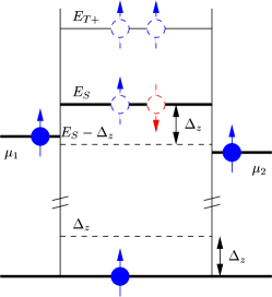
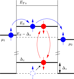
Figure 1: Closed dot (left): Chemical potentials are too small to allow an electron to tunnel onto the dot. Open dot (right): After excitation of the dot electron, the chemical potential $\mu_{1}$ is large enough for an electron of lead one to tunnel onto the dot and form the singlet state with the dot electron.

In the following we give a qualitative picture of the relevant dot states, see Fig.1, more details may be found in Ref. Engel2, . For simplicity we assume there is only one electron on the dot. With $\sigma_{z}|\!\!\uparrow\rangle=+|\!\!\uparrow\rangle$, the electron has the ground state $|\!\!\uparrow\rangle$ with energy $E_{\uparrow}=0$ and the exited state $|\!\!\downarrow\rangle$ with $E_{\downarrow}=\Delta_{z}$. If an electron tunnels onto the dot, the two electrons can form the singlet state $|S\rangle=(|\!\!\uparrow\downarrow\rangle-|\!\!\downarrow\uparrow\rangle)/\sqrt{2}$ with energy $E_{S}$ or either of the three triplet states. As the triplet state $|T_{+}\rangle=|\!\!\uparrow\uparrow\rangle$ has higher energy (for suitable magnetic field Hanson2 ), the singlet $|S\rangle$ is the ground state for two electrons on the dot. The chemical potentials are chosen such that $E_{S}>\mu_{1}=E_{S}-\Delta_{z}/2>E_{S}-\Delta_{z}>\mu_{2}=E_{S}-3\Delta_{z}/2$. Under these conditions the dot can be opened and closed for a sequential tunneling current by a spin flip induced by an ESR field:Engel2 An electron at chemical potential $\mu_{1}$ in the left lead and a dot electron in state $|\!\!\uparrow\rangle$ do not have sufficient energy to form the singlet state. If due to an ESR induced excitation the dot state is $|\!\!\downarrow\rangle$, however, less energy is required and an electron in lead one can tunnel onto the dot to form the singlet state. Tunneling onto the dot from lead two is suppressed by several orders of magnitude if the thermal energy is much lower than the energy gap even if the dot electron is in the excited state $|\!\!\downarrow\rangle$. At higher temperatures, to assure that the singlet can only be formed with the excited dot electron, one can choose spin-polarized leads. This may be achieved with several methods, see Ref. Engel2, and references therein.

Thus, within these constraints we see that the current in lead one is proportional to the probability for the dot being in the excited state, i.e. $I_{1}^{\uparrow}(t)\propto\rho_{\downarrow}$, while the current in lead two is proportional to the probability of the dot being in the singlet state, $I_{2}^{\uparrow}(t)\propto\rho_{S}$, see Ref. Engel2, .

II.1 Master equation

The traditional description of the dynamics of the dot is based on a master equation for the reduced density operator of the dot, obtained from the total density matrix $\rho_{\rm tot}(t)$ by tracing over the degrees of freedom of the leads: $\rho_{\rm dot}=Tr_{\rm leads}[\rho_{\rm tot}]$. As usual, we denote matrix elements with $\rho_{nm}=\langle n|\rho_{\rm dot}|m\rangle$ (or $\rho_{n}=\langle n|\rho_{\rm dot}|n\rangle$) and include only the three relevant dot states $n,m\in\{\uparrow,\downarrow,S\}$. We assume the dot and the leads to be uncorrelated initially, $\rho_{\rm tot}(0)=\rho_{\rm dot}(0)\otimes\rho_{\rm leads}(0)$. Starting from the von Neumann equation for the full density operator ${\dot{\rho}}_{\rm tot}=-\mathrm{i}\left[H_{\rm tot},\rho_{\rm tot}\right]$, the master equation for $\rho_{\rm dot}$ was derived in Ref. Engel2, using standard methods within the Markov approximation. Further, we will allow for an arbitrary (fixed) phase $\varphi$ of the ESR field which will play an important role in determining the spin state.

In order to eliminate the explicit time dependence emerging from the ESR field, we here base our analysis on the dot state in a rotating frame,

$$\tilde{\rho}_{\rm dot}(t)\equiv e^{\mathrm{i}\omega t|\downarrow\rangle\langle\downarrow|}\rho_{\rm dot}(t)e^{-\mathrm{i}\omega t|\downarrow\rangle\langle\downarrow|}.$$ (2)

In fact, with the exception of $\tilde{\rho}_{\downarrow\uparrow}=e^{i\omega t}\rho_{\downarrow\uparrow}$, $\tilde{\rho}_{\downarrow S}=e^{i\omega t}\rho_{\downarrow S}$ and the corresponding transposed expressions, this transformation leaves almost all matrix elements untouched.

Along the lines of the derivation in Ref. Engel2, , one finds for the dot state in the rotating frame (2) a master equation of Lindblad form.Lindblad It can be written as

$$\partial_{t}{\tilde{\rho}_{dot}}=\mathcal{L}\tilde{\rho}_{dot}\equiv-\mathrm{i}[H,\tilde{\rho}_{dot}]+\frac{1}{2}\sum_{nm}([L_{nm}\tilde{\rho}_{dot},L_{nm}^{\dagger}]+[L_{nm},\tilde{\rho}_{dot}L_{nm}^{\dagger}])$$ (3)

with the time-independent Hamiltonian (in rotating wave approximation)

$$H=(\Delta_{z}-\omega)|\!\!\downarrow\rangle\langle\downarrow|+E_{S}|S\rangle\langle S|-\frac{\Delta_{x}}{4}(e^{-\mathrm{i}\varphi}|\!\!\uparrow\rangle\langle\downarrow|+e^{\mathrm{i}\varphi}|\!\!\downarrow\rangle\langle\uparrow|)$$ (4)

and the operators $L_{nm}=\sqrt{W_{nm}}|n\rangle\langle m|$ describing incoherent transitions between levels $m$ and $n$ with a rate $W_{nm}$.

In particular, the four operators $L_{S\uparrow},L_{S\downarrow},L_{\uparrow S}$ and $L_{\downarrow S}$ describe transitions from and to the singlet state and hence correspond to the tunelling of an electron off or onto the dot. These four contributions give rise to the current in the leads and are derived from the underlying Hamiltonian (1). The rates are $W_{S\downarrow}=W_{S\downarrow}^{1}+W_{S\downarrow}^{2}$ with $W_{S\downarrow}^{l}=\gamma_{l}^{\uparrow}f_{l}(E_{S}-\Delta_{z})$ and $W_{\downarrow S}=W_{\downarrow S}^{1}+W_{\downarrow S}^{2}$ with $W_{\downarrow S}^{l}=\gamma_{l}^{\uparrow}(1-f_{l}(E_{S}-\Delta_{z}))$ where $f_{l}(E)=\left[1+e^{(E-\mu_{l})/kT}\right]^{-1}$ is the Fermi function of lead $l$. Analogously we define the rates $W_{S\uparrow}$, $W_{\uparrow S}$, $W_{S\uparrow}^{l}$, $W_{\uparrow S}^{l}$ with $\gamma_{l}^{\downarrow}$ and $f_{l}(E_{S})$. Here $\gamma_{l}^{\uparrow}=2\pi\nu_{l}^{\uparrow}|T_{l}^{\uparrow}|^{2}$ and $\gamma_{l}^{\downarrow}=2\pi\nu_{l}^{\downarrow}|T_{l}^{\downarrow}|^{2}$ are the transition rates with density of states $\nu_{l}^{\uparrow,\downarrow}$ and tunneling amplitude $T_{l}^{\uparrow,\downarrow}$.Engel2 In the limit $kT\ll\Delta_{z}$ we have $W_{S\downarrow}\approx\gamma_{1}^{\uparrow}$ and $W_{\downarrow S}\approx\gamma_{2}^{\uparrow}$, which resembles the sequential tunneling from lead one onto the dot and into lead two. Furthermore, we have $W_{S\uparrow}\approx 0$ and $W_{\uparrow S}\approx\gamma_{1}^{\downarrow}+\gamma_{2}^{\downarrow}$, because we choose $\mu_{1},\mu_{2}<E_{S}$. Throughout this paper we assume equal rates for both leads $\gamma_{1}^{\uparrow}=\gamma_{2}^{\uparrow}=\gamma^{\uparrow}$ and $\gamma_{1}^{\downarrow}=\gamma_{2}^{\downarrow}=\gamma^{\downarrow}$. Finally, we set $\gamma=\gamma^{\uparrow}=\gamma^{\downarrow}$ if the leads are not spin-polarized, and $\gamma=\gamma^{\uparrow}$, $\gamma^{\downarrow}=0$ in the case of spin-polarization.

We simulate stochastically all processes that could be observed in principle, but eventually extract the desired information from those quantities that correspond to the specific measurement scheme chosen. Quantum transitions between the dot states may be observed by monitoring the current through the dot, which is the starting point for our quantum trajectory analysis of the following Sections.

By contrast, mechanisms for incoherent spin flips (described by the operators $L_{\downarrow\uparrow}$ and $L_{\uparrow\downarrow}$) and dephasing mechanisms (described by the projectors $L_{n}\equiv L_{nn}=\sqrt{W_{n}}|n\rangle\langle n|$) are introduced on phenomenological grounds and not contained in the Hamiltonian (1). The (phenomenological) spin flip rates are assumed to satisfy the condition of detailed balance: $W_{\uparrow\downarrow}/W_{\downarrow\uparrow}=e^{\Delta_{z}/k_{B}T}$. The rates $W_{n}$ are phenomenological dephasing rates: the effect of an operator $L_{nn}$ in (3) is to kill coherences between state $|n\rangle$ and the remaining states (at a rate $W_{n}$), while leaving probabilities unaffected.

If the coupling to the leads is switched off (by an appropriate choice of the chemical potentials), the dynamics as described by the master equation (3) is that of a standard decaying two-state spin-system. Then the corresponding (intrinsic) relaxation and decoherence rates turn out to be

$$1/T_{1} = W_{\downarrow\uparrow}+W_{\uparrow\downarrow}$$ (5)

$$1/T_{2} = (1/T_{1}+W_{\uparrow}+W_{\downarrow})/2.$$

let us now turn to the dot dynamics: in terms of its coefficients, the time evolution of the dot state $\tilde{\rho}_{\rm dot}$ given by the master equation (3) reads

$$\dot{\tilde{\rho}}_{\uparrow} = -\frac{\Delta_{x}}{2}{\rm Im}(e^{-\mathrm{i}\varphi}\tilde{\rho}_{\downarrow\uparrow})-(W_{\downarrow\uparrow}+W_{S\uparrow})\tilde{\rho}_{\uparrow}+W_{\uparrow\downarrow}\tilde{\rho}_{\downarrow}+W_{\uparrow S}\tilde{\rho}_{S},$$ (6)

$$\dot{\tilde{\rho}}_{\downarrow} = \frac{\Delta_{x}}{2}{\rm Im}(e^{-\mathrm{i}\varphi}\tilde{\rho}_{\downarrow\uparrow})-(W_{\uparrow\downarrow}+W_{S\downarrow})\tilde{\rho}_{\downarrow}+W_{\downarrow\uparrow}\tilde{\rho}_{\uparrow}+W_{\downarrow S}\tilde{\rho}_{S},$$ (7)

$$\dot{\tilde{\rho}}_{S} = -(W_{\uparrow S}+W_{\downarrow S})\tilde{\rho}_{S}+W_{S\uparrow}\tilde{\rho}_{\uparrow}+W_{S\downarrow}\tilde{\rho}_{\downarrow},$$ (8)

$$\dot{\tilde{\rho}}_{\downarrow\uparrow} = -(\mathrm{i}(\Delta_{z}-\omega)+V_{\downarrow\uparrow})\tilde{\rho}_{\downarrow\uparrow}+\mathrm{i}\frac{\Delta_{x}}{4}e^{\mathrm{i}\varphi}(\tilde{\rho}_{\uparrow}-\tilde{\rho}_{\downarrow}).$$ (9)

$$\dot{\tilde{\rho}}_{S\uparrow} = -(\mathrm{i}E_{s}+V_{S\uparrow})\tilde{\rho}_{S\uparrow}-\mathrm{i}\frac{\Delta_{x}}{4}e^{\mathrm{i}\varphi}\tilde{\rho}_{S\downarrow},$$ (10)

$$\dot{\tilde{\rho}}_{S\downarrow} = -(\mathrm{i}(E_{s}-\Delta_{z}+\omega)+V_{S\downarrow})\tilde{\rho}_{S\downarrow}-\mathrm{i}\frac{\Delta_{x}}{4}e^{-\mathrm{i}\varphi}\tilde{\rho}_{S\uparrow},$$ (11)

with the effective rates

$$V_{\downarrow\uparrow} = \frac{1}{2}(W_{\downarrow\uparrow}+W_{\uparrow\downarrow}+W_{S\uparrow}+W_{S\downarrow}+W_{\downarrow}+W_{\uparrow})=\frac{1}{2}(W_{S\uparrow}+W_{S\downarrow})+\frac{1}{T_{2}},\;\;{}$$ (12)

$$V_{S\uparrow} = \frac{1}{2}(W_{\downarrow\uparrow}+W_{S\uparrow}+W_{\uparrow S}+W_{\downarrow S}+W_{S}+W_{\uparrow}),$$ (13)

$$V_{S\downarrow} = \frac{1}{2}(W_{\uparrow\downarrow}+W_{S\downarrow}+W_{\downarrow S}+W_{\uparrow S}+W_{S}+W_{\downarrow}).$$ (14)

Note that Eqs. (10, 11) are decoupled from Eqs. (6-9), and the latter are the only ones of relevance to us. They enable us to determine easily counting statistics of tunneling electrons numerically by means of the quantum trajectory method which we describe in the following Sections.

III Quantum Trajectories

One major motivation behind the development of quantum trajectory methods were experiments with with single quanta. Before these developments, naturally, ensemble experiments required simple ensemble theories. Matters changed with experiments involving single atoms, electrons or ions in traps. Continuously monitoring those systems, single quantum jumps became visible to the bare eye. A theory of continuous quantum measurement taking into account continuous measurement records of the observed environment to update the quantum state accordingly, were developed, mainly with an eye on applications in quantum optics.

Experiments on the single quantum level have reached solid state devices, as for instance electrons in quantum dots. Accordingly, the dynamics of such nano-scale quantum systems may be described adequately by quantum trajectories. In fact, it may well turn out that these methods are even more useful in solid state devices since the sensitivity of electron detectors is typically far better than that for photon detectors, on the single quantum level.

As will be explained in the following, a quantum trajectory $\rho_{c}(t)$ describes a subensemble of the full (ensemble) density operator $\rho(t)$, conditioned on a certain (stochastic) measurement record, here detection events at certain times. In this approach we determine the dynamics of an electron on a quantum dot, conditioned on the measured (stochastic) tunneling current through the dot.

Quantum trajectory methods have changed remarkably the way we think about open quantum system dynamics. While traditionally an open quantum system is described by its density operator $\rho(t)$ as in the last section, quantum trajectories describe open system dynamics taking into account certain continuous, stochastic measurement outcomes. In other words, with quantum trajectories one determines a conditioned density operator $\rho_{c}(t)$, reflecting knowledge obtained from a continuous monitoring of the environment. Sampling over all these possible measurement records, in other words, ignoring the state of the environment, one recovers the usual full ensemble $\rho(t)$. We write $\rho(t)={\cal M}[\rho_{c}(t)]$ where ${\cal M}[\ldots]$ denotes the ensemble mean over all possible measurement records with corresponding probability (see below).

The principle idea is to monitor the environment rather than ignoring, i.e.  tracing over it. In quantum optics one tries to detect photons emitted from the quantum system of interest, here we detect electrons in the leads coupled to the quantum dot.

In order to illustrate this approach, we consider a simplified open quantum system – the generalization to the quantum dot case will be obvious. This model system consists of two levels and is coupled to a continuum of states. Excitation is done by some additional mechanism, included in the Hamiltonian of the system $H$. We start with a master equation of type (3), and in this model with a single Lindblad operator $L$,

$$\dot{\rho}=\mathcal{L}\rho=-\mathrm{i}[H,\rho]+\frac{1}{2}([L\rho,L^{\dagger}]+[L,\rho L^{\dagger}]).$$ (15)

In the following we abbreviate the right hand side of the equation with the superoperator $\mathcal{L}\rho$. For concreteness, consider $L$ to describe a spontaneous transition from level $|1\rangle$ to level $|0\rangle$ with rate $W$, i.e. $L=\sqrt{W}|0\rangle\langle 1|$. We introduce the superoperator $\mathcal{S}$ such that

$$\mathcal{H}_{\rm eff}=(\mathcal{L}-\mathcal{S})\rho = -\mathrm{i}[H,\rho]-\frac{1}{2}(L^{\dagger}L\rho+\rho L^{\dagger}L)$$

$$\mathcal{S}\rho = L\rho L^{\dagger}.$$

The latter is referred to as the jump operator since its describes an emission process accompanied by the replacement of the density operator $\rho$ with the ground state: $L\rho L^{\dagger}=W\langle 1|\rho|1\rangle\;|0\rangle\langle 0|$. With $\mathcal{S}$ such defined, one obtains the quantum jump representation Carmichael of the solution of (15) in the form

$$\rho(t)=\sum_{m=0}^{\infty}\int_{0}^{t}dt_{m}\int_{0}^{t_{m}}dt_{m-1}\cdots\int_{0}^{t_{2}}dt_{1}$$

$$\times\underbrace{e^{\mathcal{H}_{\rm eff}(t-t_{m})}\mathcal{S}e^{\mathcal{H}_{\rm eff}(t_{m}-t_{m-1})}\mathcal{S}\cdots\mathcal{S}e^{\mathcal{H}_{\rm eff}t_{1}}\rho(0)}_{\bar{\rho}_{c}(t)}.$$

Clearly, the solution $\rho(t)$ is a sum (or integral, respectively) over any number $m$ of emission processes (number of projections onto $|0\rangle\langle 0|$ due to the application of the jump operator $\mathcal{S}$), appearing at any times $t_{1},t_{2},\ldots,t_{m}$ between zero and the current time $t$. One has to integrate over all corresponding (unnormalized) density operators $\bar{\rho}_{c}(t)$, as apparent from expression (III). Thus, one particular quantum trajectory is the normalized density operator $\rho_{c}(t)=\bar{\rho}_{c}(t)/tr\{\bar{\rho}_{c}(t)\}$ which describes the time evolution of the quantum system conditioned on the particular measurement record, i.e. conditioned on the number and times of emission processes. The quantum trajectory ${\rho}_{c}(t)$ occurs with probability $tr\{\bar{\rho}_{c}(t)\}$.

The normalized quantum trajectory $\rho_{c}(t)$ may be determined directly through the following prescription: at time $t+\Delta t$ the new density operator $\rho_{c}(t+\Delta t)$ is obtained in one of two ways:

First, the probability $P_{\rm jump}$, to undergo a quantum jump, i.e. to emit a quantum during the time interval $\Delta t$ is equal to the jump rate times the length of the time interval times the probability to be in the excited state: $P_{\rm jump}=W\langle 1|\rho_{c}(t)|1\rangle\Delta t=$tr$(L^{\dagger}L\rho_{c}(t))\Delta t=$tr$\{\mathcal{S}\rho_{c}(t)\}\Delta t$. If a quantum is emitted (and thus detected), i.e. a jump has occurred, the conditioned quantum state is the ground state: $\rho_{c}(t+\Delta t)=\rho_{\rm jump}=|0\rangle\langle 0|=\mathcal{S}\rho_{c}(t)/tr\{\mathcal{S}\rho_{c}(t)\}$. If however, no jump occurs, the new density operator is given by

$$\rho_{c}(t+\Delta t)=\rho_{\rm nojump}=\frac{e^{\mathcal{H}_{\rm eff}\Delta t}\rho_{c}(t)}{tr\{e^{\mathcal{H}_{\rm eff}\Delta t}\rho_{c}(t)\}}$$ (17)

as is apparent from the representation (III). In practice therefore, a quantum trajectory is obtained by determining a random number $r$ between zero and one in each time step $\Delta t$: if $r\leq P_{\rm jump}$, we set $\rho_{c}(t+\Delta t)=\rho_{\rm jump}$, if, however $r>P_{\rm jump}$, we set $\rho_{c}(t+\Delta t)=\rho_{\rm nojump}$. The full ensemble of possible states is thus given by $\rho(t+\Delta t)=P_{\rm jump}\rho_{\rm jump}+(1-P_{\rm jump})\rho_{\rm nojump}$ and indeed, one may easily verify that the right hand side equals $\mathcal{L}\rho\;\Delta t$ as expected from the master equation (15) for the full ensemble.

This branching may occur at any time step and a thus huge ensemble of different quantum trajectories may be obtained. As mentioned before, the usual reduced density operator is obtained by taking the ensemble mean. In order to obtain counting statistics as in the following sections, we simply average over many runs and obtain numerically a distribution of jump times as in a real experiment involving a single quantum system.

IV Counting statistics and state tomography

An electron spin on a quantum dot has been found useful as a memory device or a qubit for quantum information processing. Readout of the spin state through a tunneling current was investigated using a rather restricted parameter regime for which analytical results were obtained in Ref. Engel2, .

First we want to show, how the analytical results emerge very easily and directly from the quantum trajectory approach. Now we consider a regime where we can neglect spin flips, i.e. $W_{\uparrow\downarrow}=W_{\downarrow\uparrow}=\Delta_{x}=0$. As in Ref. Engel2, we choose spin-polarized leads, $\gamma^{\downarrow}=0=W_{S\uparrow}=W_{\uparrow S}$, and $\gamma^{\uparrow}=W$. In the limit $kT\ll\Delta_{z}$ we then have $W_{S\downarrow}=W_{\downarrow S}=W$. The initial state is $|\!\!\downarrow\rangle$ and since no spin flip occurs on the time scale of interest the only processes that happen are transitions between $|\!\!\downarrow\rangle$ and $|S\rangle$. The quantum jump representation (III) of this particular solution then reads

$$\rho(t)=\sum_{m=0}^{\infty}\int_{0}^{t}dt_{m}\int_{0}^{t_{m}}dt_{m-1}\cdots\int_{0}^{t_{2}}dt_{1}$$

$$\times e^{\mathcal{H}_{\rm eff}(t-t_{m})}\mathcal{S}_{ij}e^{\mathcal{H}_{\rm eff}(t_{m}-t_{m-1})}\mathcal{S}_{ji}\cdots\mathcal{S}_{S\downarrow}e^{\mathcal{H}_{\rm eff}t_{1}}\rho(0)$$

with $i,j=\downarrow,S$ and $\mathcal{S}_{ij}\rho=W|i\rangle\langle j|\rho|j\rangle\langle i|$. In the regime chosen we can write $e^{\mathcal{H}_{\rm eff}(t_{k}-t_{k-1})}\bar{\rho}_{c}(t_{k-1})=e^{-W(t_{k}-t_{k-1})}\bar{\rho}_{c}(t_{k-1})$ and then get

$$\rho(t) = e^{-Wt}\sum_{m=0}^{\infty}\int_{0}^{t}dt_{m}\int_{0}^{t_{m}}dt_{m-1}\cdots\int_{0}^{t_{2}}dt_{1}\mathcal{S}_{ij}\mathcal{S}_{ji}\cdots\mathcal{S}_{S\downarrow}\rho(0)$$ (19)

$$= e^{-Wt}\sum_{m=0}^{\infty}\frac{(Wt)^{m}}{m!}|i\rangle\underbrace{\langle j|\rho(0)|j\rangle}_{=1}\langle i|.$$ (20)

Here every operator $\mathcal{S}_{S\downarrow}$ describes an electron tunneling onto the dot from lead one and $\mathcal{S}_{\downarrow S}$ represents the hopping of an electron from the dot into lead two. Since the initial state is $|\!\!\downarrow\rangle$, the first transition is $|\!\!\downarrow\rangle\rightarrow|S\rangle$ and with a second transition back to $|\!\!\downarrow\rangle$ the first electron accumulates in lead two. A third transition to the singlet does not change the number of electrons in lead two. For a particular $q$ (number of electrons in lead two) we have to consider $m=2q$ and $m=2q+1$ and the (unnormalized) density operator for a certain $q$ at time $t$ is

$$\rho(q,t)=e^{-Wt}\sum_{m=2q}^{2q+1}\frac{(Wt)^{m}}{m!}|i\rangle\langle i|.$$ (21)

Therefore, the probability to find exactly $q$ electrons in lead two at time $t$ is

$$P(q,t)={\rm Tr}\{\rho(q,t)\}=e^{-Wt}\frac{(Wt)^{2q}}{2q!}\left(1+\frac{Wt}{2q+1}\right),$$ (22)

confirming the findings in Ref. Engel2, .

With the general quantum jump representation (III), we can overcome the limitations of the analytical result, considering arbitrary regimes and investigating the dynamics numerically. So far, the proposed measurement scheme allows one to deduce the probability to be in either of the two spin states from the current through the dot. A relative phase between $|\!\!\uparrow\rangle$ and $|\!\!\downarrow\rangle$, however, cannot be detected. In order to measure the full spin state, therefore, a tomographical measurement setup is required. Here, the freedom to apply the ESR field comes into play. We show that while applying an ESR field, phase-sensitive counting statistics result, leading to clear identification of the qubit state on the Bloch sphere. As in quantum optical setups, the full state could also be obtained with appropriate $\pi/2$-pulses, that effectively change the measurement axis. In this way, not only the $\langle\sigma_{z}\rangle$-component as in the original proposal, but also $\langle\sigma_{x}\rangle$ and $\langle\sigma_{y}\rangle$ and thus the full $\rho$ can be measured. A simpler concept, not involving these precise pulses, is to measure the spin state via counting statistics of a current through the dot in conjunction with a constant ESR field as we will show in the following. For this scheme to be successful it is crucial to control the interaction between dot and leads. We are not interested in the asymptotic, stationary distribution, but in the typical time between switching the coupling on and the first (or second, or third and so on) electron appearing in lead two. Also, it is not necessary to be able to measure the electrons in lead two with a high temporal resolution: one can switch off the coupling between dot and lead two after a certain time $t$ and has any time thereafter to collect the electrons in lead two. We note that different measurement schemes are possible. Since an electron tunneling onto the dot already carries the information about the spin of the dot electron, one could abandon lead two altogether and try to monitor the number of electrons on the quantum dot, e.g. with a quantum point contact. Our proposal for quantum state tomography could be transferred to other setups as well, as for recent experiments.Elzerman3 ; Jelezko

We assume that the dot is in a given initial state at $t=0$, when the coupling to the leads is switched on. Then we measure the number of electrons tunneling into lead two. According to the quantum trajectory approach we calculate the evolution of the density matrix. Every jump from $|S\rangle$ to $|\!\!\downarrow\rangle$ or $|\!\!\uparrow\rangle$ indicates that an electron tunneled out of the dot. At very low temperatures, as assumed throughout this paper, the probability of tunneling into lead two is close to unity, while tunneling into lead one is very unlikely.

A single run of the stochastic evolution will display emission processes, i.e. contributions to the current, at certain random times. Counting the corresponding number of quanta in lead two as a function of time for a large ensemble of quantum trajectories allows us to determine the probability $P(q,t)$ of finding exactly $q$ electrons in lead two at time $t$ for a given initial state of the dot. Such counting distributions are displayed in the following Figures. We stress again that experimentally, it is not required to be able to measure these arrival times with a high resolution. One simply switches off the coupling between dot and lead two after a given time $t$. Then one has any time to determine the number of electrons in lead two. Our numerical procedure can be applied to any parameter values and any time dependence of the driving ESR field. For the regime chosen in Ref. Engel2, , we recover the analytical results (22) to a high degree of precision, as will be shown below.

Let us now turn to the probability distributions $P(q,t)$ of finding exactly $q$ electrons in lead two at time $t$ for a given initial state $\rho$. As we will show, by employing the ESR field, the counting statistics allows to clearly identify the full two-level state, including the relative phase. As usual, we choose to parametrise the latter through the coordinates on the Bloch sphere: the spin up state $|\!\!\uparrow\rangle$ corresponds to the north pole with $r=1,\theta=0^{\circ}$, while the spin down state $|\!\!\downarrow\rangle$ has coordinates $r=1,\theta=180^{\circ}$. The full mixture $\rho_{0}=\frac{1}{2}\left(|\!\!\uparrow\rangle\langle\uparrow\!\!|+|\!\!\downarrow\rangle\langle\downarrow\!\!|\right)$ corresponds to the center of the Bloch sphere, $r=0$ while coherent superpositions $\psi=(|\!\!\uparrow\rangle+e^{i\phi}|\!\!\downarrow\rangle)/\sqrt{2}$ live on the equator with $r=1,\theta=90^{\circ},\phi$.

Figure 2: Counting statistics $P(q=1,t)$ for the first electron with initial spin up state (dashed ,$r=1,\theta=0$), spin down state (dotted, $r=1,\theta=180^{\circ}$) and the totally mixed state (full curve, $r=0$). The respective coordinates refer to the Bloch sphere. The inset shows the same curves with the counting statistics of the fully mixed state subtracted. Parameters chosen are $\Delta_{x}=2\gamma=4(\Delta_{z}-\omega)=2\times 10^{6}s^{-1},T=20mK,B_{z}=12T$

In order to be able to use these counting statistics as a method for spin state tomography, the right choice of parameters is crucial. From Eqs. (6,7,8,9) it is obvious that coherences in the two-level state can only be transferred to measurable probabilities through the coupling introduced by the ESR field of magnitude $\Delta_{x}$. On the other hand, a large value of $\Delta_{x}$ leads to Rabi oscillations and thus prevents us to distinguish clearly the two fundamental $|\!\!\uparrow\rangle$ and $|\!\!\downarrow\rangle$ states on a time scale large compared with the Rabi frequency $\Delta_{x}/2$. Closer inspection of Eqs. (6, 7, 9) and numerical evidence shows that a good phase sensitivity with preserved distinguishability of $|\!\!\uparrow\rangle$ and $|\!\!\downarrow\rangle$ is achieved through the choices

$$\frac{\Delta_{x}}{2} \approx W_{S\downarrow}$$ (23)

$$\Delta_{z}-\omega \approx \frac{\Delta_{x}}{4}.$$

Physically, the first condition (on the ESR field strength) means that the spin should not be flipped to fast (compared with the measurement time scale $W_{S\downarrow}$) but still, the ESR field had time enough to make the coherences felt. The second condition (on the ESR field frequency) ensures that the method is sensitive to all values of the phase angle $\phi$.

In Fig. 2 we show counting statistics for the first electron $P(q=1,t)$ to appear in lead two. We choose the transition rate $\gamma=10^{6}s^{-1}$, an experimentally accessible magnetic field strengthlossprivate of the ESR field $B_{x}\approx 5.16G$, a slightly detuned ESR field frequency $\Delta_{z}-\omega=5\times 10^{5}s^{-1}$, a temperature $T=20mK$, and a static magnetic field of strength $B_{z}=12T$. For the ESR field to start at zero we choose the fixed phase $\varphi=3\pi/2$. Furthermore, we assume $T_{1}=10^{-4}s$ and $T_{2}=10^{-5}s$ for the intrinsic relaxation and decoherence times. All Figures are calculated with an ensemble of 50000 trajectories.

The spin down state only allows for electrons to tunnel through the dot, which is clearly visible in the counting statistics: if the spin starts off in the spin up state (dotted curve) the time to measure the first electron is delayed compared to the mixture and even more so compared to the spin down state. Eventually, however, due to the presence of the ESR field, a sufficient spin down component will be established allowing electrons to tunnel through the dot. Still, both states are clearly distinguishable through their counting statistics.

Figure 3: Counting statistics $P(q=1,t)$ for eight coherent superpositions $\psi=(|\!\!\uparrow\rangle+e^{i\phi}|\!\!\downarrow\rangle)/\sqrt{2}$ along the equator of the Bloch sphere ($r=1,\theta=90^{\circ}$, various angles $\phi$) and the fully mixed state ($r=0$, full line). The inset shows the same curves with $P(q=1,t)$ of the full mixture subtracted. Same parameters as in Fig. 2.

Not only are counting statistics useful to distinguish between up and down state. The arrival time distribution also differentiates between coherent superpositions and mixtures. In conjunction with the ESR field one may even determine the phase of coherent superpositions of type $\psi=(|\!\!\uparrow\rangle+e^{-i\phi}|\!\!\downarrow\rangle)/\sqrt{2}$ as displayed in Fig. 2. The full line corresponds to $P(q=1,t)$ of a fully mixed initial state ($r=0$), the dashed and dotted lines correspond to eight coherent superpositions along the equator of the Bloch sphere. Clearly, $P(q=1,t)$ shows different behavior for different angles $\phi$ and may thus be used to fully identify the initial state.

As we have seen, with these choices for the ESR field, not only we can distinguish $|\!\!\uparrow\rangle$ from $|\!\!\downarrow\rangle$ through counting statistics as in Fig. 2. We are in a position to fully determine the two-level state – in particular, it is possible to clearly distinguish a coherent superposition of $|\!\!\uparrow\rangle$ from $|\!\!\downarrow\rangle$ from the mixture of the two, as shown in Fig. 3.

The insets of Figs. 2 and 3 reveal an interesting structure underlying the shapes of $P(q=1,t)$: Once the counting distribution of the full mixture ($r=0$) is subtracted, statistics of states corresponding to opposite points on the Bloch sphere appear as mirror-images of each other, as highlighted in Figs. 4 and 5. In these Figures we display the counting statistics $P(q=1,t)$ for four pairs of opposite initial states along the equator of the Bloch sphere and clearly confirm the observations just mentioned. A linear combination of initial states leads to a linear combination of counting statistics in the ensemble and thus to this symmetry. Still, each curve in itself seems complicated enough to underline the importance of our numerical approach. Using the quantum trajectory method, any time dependence of the fields and any choice of parameters is possible.

Figure 4: Graphs taken from Fig. 3 for four pairs of opposite states along the equator of the Bloch sphere.

Figure 5: Same as Fig. 4 with $P(q=1,t)$ of the full mixture subtracted. We clearly see the symmetry of the curves for opposite states on the Bloch sphere.

The more mixed the initial state, i.e. the smaller $r<1$ on the Bloch sphere, the closer the curve to the curve of the fully mixed state. It is also worth noting that we keep the initial phase $\varphi$ of the ESR pulse fixed for all calculations. An average over all possible phases would indeed lead to the graph of the fully mixed state, irrespective of the phase $\phi$ of the initial quantum state.

IV.1 Higher order statistics and $q=0$

We close this section by pointing out that also higher order counting statistics ($q=2,3,4,5$) display state-sensitive behaviour – if only less pronounced. This is quite obvious since a delayed first tunneling event shifts the starting time for the following electrons. For $q=0$, the difference between the counting statistics for various initial states is well pronounced. In this latter case, however, the curves do not cross which diminishes the distinguishability of states and the best choice for that is $q=1$. As displayed in Fig. 6, higher-order counting statistics $P(q,t)$ still distinguishes between the fully mixed state ($r=0$) and a coherent superposition ($r=1,\theta=90^{\circ}$).

Figure 6: Counting statistics of exactly zero, one, five electrons tunneling through the dot. Evidently, if less pronounced, all counting statistics $P(q,t)\;(q=0,1,\ldots,5,\ldots)$ carry information about the initial quantum state.

IV.2 The role of spin-polarized leads

The original proposal for the spin state readout was based on spin-polarized leads in order to clearly distinguish the two states $|\!\!\uparrow\rangle$, $|\!\!\downarrow\rangle$ by a single shot measurement. As the counting statistics require an ensemble measurement, our results suggest that spin polarization is not required for those – not even advantageous, in fact. In Fig. 7 we display counting statistics $P(q=1,t)$ for spin-polarized leads (only spin-up electrons in the leads, i.e. $\gamma^{\downarrow}=0$). We notice only marginal differences compared to the case of unpolarized leads (Fig. 3).

For large times, it is more likely to observe precisely one electron in the case of unpolarized leads. The reason for this behaviour is the fact that for unpolarized leads, there is also the possibility that the spin-up electron on the dot (rather than the spin-down electron entering the dot) may tunnel out of the dot. Then the dot is in the ground state and therefore closed for the tunneling of another electron. It is only after the ESR field had time to populate the excited state that a second electron may tunnel through the dot. In fact, it turns out that this mechanism is the preferred tunneling event: for the parameters of Fig. 2 we find $W_{\downarrow S}=1\times 10^{6}s^{-1}$ and $W_{\uparrow S}=2\times 10^{6}s^{-1}$.

Figure 7: Same graph as Fig. 3. Here, however using spin-polarized leads with $\gamma^{\uparrow}=1\times 10^{6}s^{-1}$, $\gamma^{\downarrow}=0$.

V Relaxation and decoherence times

Our proposed setup including the ESR field may be used to determine the intrinsic relaxation time $T_{1}$ and decoherence time $T_{2}$ of the qubit in the time domain. Tuning the tunneling rate over a wide range (and adjusting the ESR field strength and frequency according to conditions (23), one can easily see the effect of decoherence and relaxation. In the series of graphs in Fig. 8 we show counting statistics for the $|\!\!\downarrow\rangle$ and $|\!\!\uparrow\rangle$-state, for the full mixture and for two coherent superpositions (states on the equator of the Bloch sphere). Clearly, for large tunneling rate (left graph, (a)), all states may be distinguished. The third graph (c) shows a regime where decoherence has fully set in: while the states $|\!\!\downarrow\rangle$ and $|\!\!\uparrow\rangle$-state remain essentially unaffected, the counting statistics of the coherent superpositions collapse onto the curve of the full mixture. In other words, while no relaxation has set in yet, coherences between the states $|\!\!\downarrow\rangle$ and $|\!\!\uparrow\rangle$ have disappeared. Decreasing the tunneling rate even further, counting statistics finally reveal the relaxation time: eventually, the initial states $|\!\!\downarrow\rangle$ and $|\!\!\uparrow\rangle$ may no longer be distinguished, i.e. the relaxation has taken place.

Figure 8: Measurement of a variety of states ($|\!\!\uparrow\rangle$, $|\!\!\downarrow\rangle$, coherent superposition) facilitates an estimate of $T_{2}$ and $T_{1}$.

VI Single shot readout

Counting statistics was used in Ref. Engel2, to determine the measurement time and measurement efficiency. It was shown that after about ten times the tunneling time, the spin state on the dot could be determined to be either $|\!\!\uparrow\rangle$ or $|\!\!\downarrow\rangle$ with close to 100% efficiency, even if only a single measurement is made (provided it was either $|\!\!\uparrow\rangle$ or $|\!\!\downarrow\rangle$). Crucially, these results are based on spin-polarized leads. Without spin-polarization the determination of the dot state with a single measurement appears problematic. The reason is that an electron may tunnel from the quantum dot back into lead one rather than into lead two. In fact, since in the case of unpolarized leads there are three ways for an electron to leave the dot: it may tunnel from lead one onto the dot and further into lead two (transition $|S\rangle\rightarrow|\!\!\downarrow\rangle$) or the electrons interchange the roles and the one residing on the dot tunnels into either of the two leads ($|S\rangle\rightarrow|\!\!\uparrow\rangle$). The latter two possibilities are almost of same probability and therefore with a probability of about one third a tunneling process has taken place without having been observed in lead two. In other words, with a probability of two thirds only we can claim that without detecting an electron in lead two after sufficient time the spin state on the dot was $|\!\!\uparrow\rangle$.

In order to overcome this problem we propose to measure the number of electrons on the dot with a quantum point contact and recent experiments Elzerman3 show that such a concept may work. If an electron tunnels onto the dot it confirms that the state was $|\!\!\downarrow\rangle$ and if it stays there sufficiently long the QPC as electrometer recognizes the charge. Since the projection takes place if an electron tunnels onto the dot, the second lead could even be omitted and then the dot electron would tunnel into lead one. For clarity in the following argument, however, we do not change our setup and leave lead two as before.

With the help of the QPC it is possible to measure the state of a single electron spin with an efficiency of almost 100% after about ten times the tunneling time, as for polarized leads as shown in Fig. 10. Note that for this scheme to work, it is important that the time resolution of the point contact measurement has to be better than the inverse tunneling rate $\gamma^{-1}$ to ensure the detection of the tunneled electron on the dot.

Figure 9: With spin-polarized (s-p) leads, a detection of an electron in lead two after about 10 times the tunneling time ensures to almost 100% that the initial dot state was $|\!\!\downarrow\rangle$. Without spin polarization, only a probability of about two thirds may be achieved due to the possibility of the electron to tunnel into lead one. The numerical curve accounts for spin relaxation and therefore differs slightly from the analytical result. Without spin relaxation no difference can be seen. Parameters as in Fig. 2 respectively Fig. 7, but without ESR-field.

Figure 10: Measuring the probability to find two electrons on the dot one may determine the dot state with 100% efficiency. Clearly, the time resolution has to be better than the typical time the two electrons stay on the dot, i.e. better than $\gamma^{-1}$. Here $P_{{\rm nt}}^{[0,t]}$ is the probability that no tunneling event occurred in the whole interval $[0,t]$ and $P_{{\rm dot},\rho_{0}}(q,t)$ is the probability to find exactly $q$ electrons on the dot at time $t$. The initial state was always $|\!\!\downarrow\rangle$, parameters as in Fig. 9.

VII Conclusion

We use quantum trajectory methods to investigate counting statistics of electrons tunneling through a quantum dot. We show how an additional ESR field may actively be used to perform a full “state tomography”. Applying the field during the measurement allows one to clearly identify the coherences between the two superposed states. We discuss the relevance of our findings for determining intrinsic relaxation and decoherence times of electron spin states in quantum dots – in the time domain. Based on a quantum point contact we propose a scheme for single-shot readout without the need for spin-polarized leads. Similarities of the investigated quantum dot to three-level systems in quantum optics (e.g. so-called “V”-systems) are evident. We underline these connections by applying the quantum jump method in order to unravel the dynamics of the full density operator $\rho(t)$ into subensembles $\rho_{c}(t)$ corresponding to certain measurement records in the leads. Thus, we describe the conditioned time evolution of the spin state, given a certain measurement record, as in actual experiments with single quanta.

We believe that such connections between methods of quantum optics and mesoscopic devices will prove more and more useful in the future as nanotechnology achieves further breakthroughs in the coherent manipulation of quantum dynamics in solid state devices.

- (1) M. A. Nielsen and I. D. Chuang, Quantum Computation and Quantum Information, Cambridge, (2000).
- (2) A. Leggett, B. Ruggerio, and P. Silvestrini (eds.), Quantum Computing and Quantum Bits in Mesoscopic Systems, Kluwer (2003).
- (3) D. Vion, A. Aassime, A. Cottet, P. Joyez, H. Pothier, C. Urbina, D. Esteve, and M. H. Devoret, Science 296, 886 (2002).
- (4) C. P. Heij, D. C. Dixon, C. H. van der Wal, P. Hadley, and J. E. Mooij, Phys. Rev. B 67, 144512 (2003).
- (5) O. Astafiev, Yu. A. Pashkin, T. Yamamoto, Y. Nakamura, and J. S. Tsai, Phys. Rev. B 69, 180507 (2004).
- (6) F. Jelezko, T. Gaebel, I. Popa, A. Gruber, and J. Wrachtrup , Phys. Rev. Lett. 92, 076401 (2004).
- (7) D. Loss and D. P. DiVincenzo, Phys. Rev. A 57, 120 (1998).
- (8) P. Recher, E. V. Sukhorukov, and D. Loss, Phys. Rev. Lett. 85, 1962 (2000).
- (9) H.-A. Engel and D. Loss, Phys. Rev. Lett. 86, 4648 (2001).
- (10) H.-A. Engel and D. Loss, Phys. Rev. B 65, 195321 (2002).
- (11) H.-A. Engel, V. Golovach, D. Loss, L. M. K. Vandersypen, J. M. Elzerman, R. Hanson, and L. P. Kouwenhoven, cond-mat/0309023 (unpublished).
- (12) L. M. K. Vandersypen, R. Hanson, L. H. Willems van Beveren, J. M. Elzerman, J. S. Greidanus, S. De Franceschi, and L. P. Kouwenhoven, in Quantum Computing and Quantum Bits in Mesoscopic Systems, edited by A. Leggett, B. Ruggerio, and P. Silvestrini, (Kluwer Academic/Plenum, New York, 2003); see also quant-ph/0207059, (2002).
- (13) J. M. Elzerman, R. Hanson, J. S. Greidanus, L. H. Willems van Beveren, S. De Franceschi, L. M. K. Vandersypen, S. Tarucha, and L. P. Kouwenhoven, Phys. Rev. B 67, 161308(R) (2003).
- (14) R. Hanson, B. Witkamp, L. M. K. Vandersypen, L. H. Willems van Beveren, J. M. Elzerman, and L. P. Kouwenhoven , Phys. Rev. Lett. 91, 196802 (2003).
- (15) R. Hanson, L. M. K. Vandersypen, L. H. Willems van Beveren, J. M. Elzerman, I. T. Vink, and L. P. Kouwenhoven, cond-mat/0311414 (unpublished).
- (16) J. M. Elzerman, R. Hanson, L. H. Willems van Beveren, L. M. K. Vandersypen, and L. P. Kouwenhoven , Appl. Phys. Lett. 84, 4617 (2004).
- (17) J. M. Elzerman, R. Hanson, L. H. Willems van Beveren, B. Witkamp, L. M. K. Vandersypen, and L. P. Kouwenhoven, Nature 430, 431 (2004).
- (18) D. A. Bagrets and Yu. V. Nazarov, Phys. Rev. B 67, 085316 (2003).
- (19) A. Shnirman and G. Schön, Phys. Rev. B 57, 15400 (1998).
- (20) W. Lu, Z. Ji, L. Pfeiffer, K. W. West, and A. J. Rimberg , Nature 423, 422 (2003).
- (21) L. M. K. Vandersypen, J. M. Elzerman, R. N. Schouten, L. H. Willems van Beveren, R. Hanson, and L. P. Kouwenhoven, cond-mat/0407121 (unpublished).
- (22) Yu. Makhlin, G. Schön, and A. Shnirman, Phys. Rev. Lett. 85, 4578 (2000).
- (23) H. J. Carmichael, An Open Systems Approach to Quantum Optics, Lecture Notes in Physics (Springer, Berlin, 1993).
- (24) M. B. Plenio, P. L. Knight, Rev. Mod. Phys. 70, 101 (1998).
- (25) R. Ruskov and A. N. Korotkov, Phys. Rev. B 67, 241305(R) (2003).
- (26) H.-S. Goan and G. J. Milburn, Phys. Rev. B 64, 235307 (2001).
- (27) G. Alber, Th. Beth, Ch. Charnes, A. Delgado, M. Grassl, and M. Mussinger, Phys. Rev. A 68, 012316 (2003).
- (28) H. M. Wiseman, Phys. Rev. A 49, 2133 (1994).
- (29) G. Lindblad, Comm. Math. Phys. 48, 119 (1976).
- (30) D. Loss, priv. comm.