Complex systems Systems obeying scaling laws Fluctuation phenomena, random processes, noise, and Brownian motion Economics; econophysics, financial markets, business and management

Multiscaling and non-universality in fluctuations of driven complex systems

Abstract

For many externally driven complex systems neither the noisy driving force, nor the internal dynamics are a priori known. Here we focus on systems for which the time dependent activity of a large number of components can be monitored, allowing us to separate each signal into a component attributed to the external driving force and one to the internal dynamics. We propose a formalism to capture the potential multiscaling in the fluctuations and apply it to the high frequency trading records of the New York Stock Exchange. We find that on the time scale of minutes the dynamics is governed by internal processes, while on a daily or longer scale the external factors dominate. This transition from internal to external dynamics induces systematic changes in the scaling exponents, offering direct evidence of non-universality in the system.

While it is hard to find a generally accepted definition of complex systems, most systems that are colloquially labeled ”complex” include a large number of interacting constituents (or nodes) whose collective dynamics leads to emergent spatial and/or temporal structures [1]. The most studied examples that fit this paradigm include the cell, vehicular traffic or the World-Wide-Web [2]. Very often these systems operate far from equilibrium and under the influence of an external driving force. Yet, typically the mechanisms governing the internal dynamics of these systems are not a priori known and even the driving force is not necessarily under the observer’s control. Moreover, the separation of the system from its environment is often arbitrary, making difficult to systematically distinguish the internal from the external degrees of freedom.

With the improvement of the measurement and information processing tools an increasing number of systems can be monitored through multichannel measurements, offering the possibility to record and characterize the simultaneous time dependent behavior of many of the system’s constituents. These advances in observational techniques offer an important scientific challenge: Can we design systematic methods that, taking advantage of the new datasets, can help us to map out the interactions and the dynamics of various complex systems? Considering the large number of constituents and the complexity of the behavior displayed by them the above task is a truly ambitious undertaking, thus even partial progress is of major potential significance.

Concepts like scaling, multiscaling and universality [3] have been found extremely useful in the characterization of complex phenomena, as they offer general relationships, leading to organizing and systematic categorization principles. Indeed, recent measurements focusing on the fluctuations at the “nodes” of several complex systems [4] indicate that the relationship between the standard deviation $\sigma_{i}$ and time average $\left\langle f_{i}\right\rangle$ of the $f_{i}(t)$ signal capturing the time dependent activity of node $i=1,\dots,N$ follows the scaling law

$$\sigma\propto\langle f\rangle^{\alpha}.$$ (1)

Yet, this finding leaves a number of important questions unanswered. For example, the measurements indicate that real systems belong to one of the two extreme universality classes characterized by either $\alpha\approx 1/2$ (observed for the Internet and computer chip) or $\alpha\approx 1$ (highway traffic, river network and World-Wide-Web), the former describing an endogenous, while the latter an exogenous dominance in the fluctuations. Finding systems that display internal organizing principles leading to different exponents from these two extreme values would significantly enrich our understanding of complex dynamics. Furthermore, universality in statistical physics is more than mere numerical agreement of exponents: In critical phenomena [5] whole scaling functions are expected to be universal. A natural question in this context can be formulated as follows: Are the distributions of the fluctuations characterized by universal scaling functions? In this sense a signature of non-universality would be if some systems showed multifractality while others did not. Indeed, in the systems investigated thus far multiscaling appeared to be absent [6]. A major goal of this paper is to introduce the computational tools to uncover potential multiscaling in real systems. Finally, we apply these tools to the stock market, offering direct evidence of both non-universal exponents and multiscaling.

To capture the dynamics of systems that can be monitored through several channels we decompose the signals into two components, that we will call the external and the internal part [7]. For this we define the system’s global activity $F(t)$ as a sum over the activity of all elements

$$F(t)=\sum_{i}f_{i}(t).$$ (2)

As $F(t)$ characterizes the common trends in the systems’s activity, in (2) the individual, independent fluctuations of the components are averaged out. The components are expected to follow this ”external” or averaged trend (which itself may be noisy), while the fluctuations around $F(t)$ are of ”internal” origin, driven by interactions among the system’s components. For a wide variety of cases the total activity $f_{i}(t)$ of node $i$ can be split into an external activity defined as

$$f_{i}^{ext}(t)=\frac{\left\langle f_{i}\right\rangle}{\left\langle F\right\rangle}F(t),$$ (3)

representing node $i$’s expected share of the global activity $F(t)$, and the deviations or internal activity is given by

$$f_{i}^{int}(t)=f_{i}(t)-\frac{\left\langle f_{i}\right\rangle}{\left\langle F\right\rangle}F(t),$$ (4)

where $\left\langle\cdot\right\rangle$ denotes temporal average [8], while (4) the fluctuating component of a node’s activity. By definition, $\left\langle f_{i}^{int}\right\rangle=0$. However, (3) contains the expected changes in the node’s activity, given the overall changes in the system’s activity. If the system is closed, then $F(t)$ is time independent. Thus there are no changes in the external component $f_{i}^{ext}(t)$ either.

The standard deviation $\sigma^{(\ell)}_{i}$ of the activity of the $i$th component is

$$\sigma^{(\ell)}_{i}=\sqrt{\left\langle\left(f_{i}^{(\ell)}-\left\langle f_{i}^{(\ell)}\right\rangle\right)^{2}\right\rangle},$$ (5)

where the label $(\ell)$ represents tot, int or ext, indicating that $\sigma_{i}$ is calculated from the total, internal or external signal, respectively. We will everywhere omit $(\ell)$ for the total case.

In order to investigate the multiscaling behavior of the fluctuations of total noise we propose the multiscaling relation:

$$\left\langle\left|f_{i}-\left\langle f_{i}\right\rangle\right|^{q}\right\rangle=C_{F}^{q}(\Delta t,q)\left\langle f_{i}\right\rangle^{q\alpha(q)}.$$ (6)

This means that all $q$th order central moments of activity, which characterize fluctuations around the mean behavior, scale as power-laws with the mean total activity of the same element. In this notation, $\alpha=\alpha(2)$. Note that analogous definitions can be given for the internal and the external case. In particular, as $\left\langle\left|f_{i}^{ext}\right|^{q}\right\rangle\equiv{\left\langle f_{i}\right\rangle^{q}},$ for external activity we have $\alpha(q;ext)\equiv 1$ [see (3)], indicating that multiscaling can be present only in the internal or total fluctuations. In (6) $\alpha(q)$ is a formal analogue to the generalized dimensions $H(q)$ for multifractal or multiaffine time series [10], defined as

$$\left\langle\left|f_{i}-\left\langle f_{i}\right\rangle\right|^{q}\right\rangle=C_{T}^{q}(i,q)\Delta t^{qH(i,q)},$$ (7)

where $\Delta t$ is the time above which the averages are to be taken. Combining (6) and (7) one can eliminate a variable, obtaining:

$$\frac{\left\langle f_{i;\Delta t}\right\rangle^{\alpha(\Delta t,q)}}{\left\langle f_{i;\Delta t}\right\rangle^{\alpha(\Delta t,q^{\prime})H(i,q)/H(i,q^{\prime})}}\frac{C_{F}(\Delta t,q)}{C_{F}(\Delta t,q^{\prime})^{H(i,q)/H(i,q^{\prime})}}=\frac{C_{T}(i,q)}{C_{T}(i,q^{\prime})^{H(i,q)/H(i,q^{\prime})}}.$$ (8)

Here the r.h.s. does not depend on $\Delta t$, thus the l.h.s. should not either. Information on the temporal scaling goes into the r.h.s. in form of the exponent ratios $H(q)/H(q^{\prime})$. However, if the time series does not show multifractality, i.e., $H(q)=H(q^{\prime})$ then the simple moment ratios from (6) should not depend on the the averaging time:

$$\frac{C_{F}(\Delta t,q)\left\langle f_{i;\Delta t}\right\rangle^{\alpha(\Delta t,q)}}{C_{F}(\Delta t,q^{\prime})\left\langle f_{i;\Delta t}\right\rangle^{\alpha(\Delta t,q^{\prime})}}=\frac{C_{T}(i,q)}{C_{T}(i,q^{\prime})}.$$ (9)

Let us turn to an example where the tools introduced above prove useful. In the study of the financial market as a complex system statistical physics concepts turned out to be very powerful [11]. Enormous amount of data is available as every transaction is recorded on the stock market. A natural choice of constituents here are the stocks of firms that are publicly traded. In order to keep the analogy with previously studied cases we have chosen the flow as the signals. On a given time horizon $\Delta t$, let the (total) activity or flow of the $i$th stock at time $t$ be

$$f_{i}^{\Delta t}(t)=\sum_{\tau\in[t,t+\Delta t]}Y_{i}(\tau)V_{i}(\tau),$$ (10)

where $\tau$ runs for all trades of the $i$th stock in the given interval. This corresponds to the coarse-graining of the individual events, or the so-called tick-by-tick data. $Y_{i}(\tau)$ is the price and $V_{i}(\tau)$ is the traded volume for the trade at time $\tau$ [12]. We used data with a minute resolution where the price within the minute was that of the last trading minute (which causes a negligible error). Hence, $f_{i}^{\Delta t}(t)$ gives the total traded value of stock $i$ between times $t$ and $t+\Delta t$. $\Delta t$ can be chosen as any multiple of $1$ minute, and $t=0,\Delta t,2\Delta t,\dots$. In the following for simplicity of notation we will omit $\Delta t$’s where they are kept constant, only indicating their value once.

For empirical analysis we used the TAQ database [13] of the New York Stock Exchange for the period of 2000-2002, which after some filtering[14] contains $N=2200$ stocks.

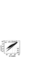
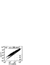
The $\alpha(q)$ scaling exponents were measured for fixed $\Delta t$, examples being shown in Fig. 1. The first striking observation is that for the second moment we find power law behavior over five orders of magnitude with an exponent which is significantly different from both 1/2 and 1. Second, we find multiscaling (i.e., a dependence of $\alpha(q)$ on $q$, except for the trivial case of external activity), as shown in Fig. 2. Furthermore, the exponents show a strong dependence on the time horizon $\Delta t$.

         

Figure 1: Scaling of $q=2$ central moments of activities and fitted linear trends. (a) $\Delta t=10$ minutes. $\alpha(2;tot)\approx\alpha(2;int)=0.773\pm 0.003$. (b) $\Delta t=390$ minutes = $1$ trading day. $\alpha(2;tot)\approx\alpha(2;int)=0.885\pm 0.005$. Errors are estimated from the linear fit on the log-log plot. Note that although the errors are very low due to the large number of data points, there is pronounced unexplained variance around the expected scaling of total and internal noise. This can be reduced significantly if one takes the system structure (in our case the clustering of stocks into market sectors) into account [9].

   

Figure 2: The $\alpha(q)$ multiscaling exponents for all three types of activity. $\alpha(q;ext)\equiv 1$. (a) $\Delta t=10$ minutes. (b) $\Delta t=390$ minutes = $1$ trading day.

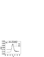
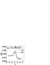
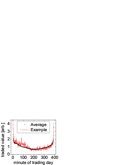
In the activity (10) there are two sources of external impact, a random and a regular part. The latter is manifest in, e.g., different kinds of seasonalities and intraday patterns. Since we are interested in the fluctuations it is natural to detrend the data from such regular contributions. In this respect intraday patterns are particularly strong [11]: At the beginning and end of the trading day the activity is anomalously high. In addition, one finds a small irregularity in activity right after 10 a.m., which is a typical time for news arrival. The pattern, averaged for all full-length days in our dataset, is shown in Fig. 3 which is used for detrending, achieved by dividing traded values by the respective values of the trend pattern.

Figure 3: The average intraday pattern of trading activity. The activity time series of one example day is given for comparison.

We measured the scaling exponents $\alpha$, using fits similar to those in Fig. 1. Simultaneously, we calculated the values of $\log(\eta(\Delta t))$ (with $\eta=\sigma_{ext}/\sigma_{int}$) averaged over all stocks. Both results are shown in Fig. 4, indicating a significant $\Delta t$ dependence. One finds that as we move from the minute scale to the weekly scale, the nature of fluctuations changes gradually toward the externally driven limit. This is in correspondence with results for the $\eta$ ratio (see Fig. 4(b)). Detrending of the data causes a little systematic decrease in $\alpha$ values for time horizons less than one day.

Figure 4: (a) Values of $\alpha$ as a function of the time scale $\Delta t$. There is a clear tendency present. The exponent grows from a lower value corresponding to the dominance of internal dynamics to nearly $1$, which characterizes externally driven systems. (b) The ratio of the standard deviation of fluctuations originating from external and internal sources. Raw data shows an anomalous behavior, the result of peaks in trading activity at the beginning and the end of each day of trading. Results for data detrended with the average of this daily pattern show an effect similar to the one in the behavior of the exponent $\alpha$. In the $\Delta t=1\dots 390$ minutes $=1$ day interval, there is a faster increase in the contribution of external fluctuations. Beyond the scale of a few days this tendency saturates.

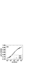
An anomalous non-monotonicity is present in the raw data [see Fig. 4(b)], while for the detrended data, we recover the expected tendency: As $\Delta t$ increases, the external driving force gets stronger. The range of $\eta$ is similar to that in [4]. We find, that for $\Delta t$’s larger than a few days, the external contribution to fluctuations saturates.

Figure 5: Histogram of the ratios of the internal and external standard deviations for all stocks, both for raw and detrended time series. The comparison shows, that external influence is stronger on a daily time scale than for fine resolution data. (a) $\Delta t=10$ minutes. Detrending with the intraday pattern removes the spurious external driving force due to daily peaks in activity. This decreases the measured external contribution in fluctuations. (b) $\Delta t=390$ minutes = $1$ trading day. Detrending does not change behavior measured on a daily (or longer) scale.

As we change the time scales ($\Delta t=1$ minute$\dots 2$ weeks) we observe a transition between two limits. With decreasing $\Delta t$, we get closer to the limiting endogenous behavior $\alpha=\alpha_{int}<1$, and $\eta\ll 1$. Yet, Fig. 4(a) indicates, that even the limiting value $\alpha^{*}_{int}$ should significantly differ from $1/2$ measured in several systems[4, 15]. This suggests that despite earlier observations [4] the behavior $\alpha^{*}_{int}=1/2$ is not universal, although the mechanism responsible for this non-trivial scaling is unknown. Furthermore, we observe a continuous dependence of the exponent $\alpha_{int}$ on $\Delta t$ with scaling spanning over five orders of magnitude, indicating that the observed exponents are likely not due to finite size crossover phenomena. With increasing $\Delta t$ there is a growing role of external forces, and beyond the daily scale we reach the exogenous limit, where $\alpha\rightarrow 1$ and $\eta\sim 0.20$. In this limit the dynamics is dominated by the external driving force. This mechanism is behind the so called Epps-effect [16], namely that in high frequency data the cross correlations between stock data are much less pronounced than in, say, daily ones: Correlations reflect the similarities in how different stocks react to external effects and this is covered for short time horizons by noisy internal dynamics.

These results offer a coherent qualitative picture about market dynamics. The impact of incoming news needs a finite time to diffuse. Hence, on short time scales, the response to them is small. The factor that determines the fluctuations of trading activity is internal: it is the trading mechanism itself. On daily or longer scales, however, the internal fluctuations have smaller importance, and the market tends to move with the global activity. In periods of “business as usual” the natural human scale of one day seems to be needed to reach a kind of coherence: News and trends can be evaluated, informations are exchanged and collective decisions are made. Interestingly, the scaling of asset return distributions [11] also breaks down on the scale of one day, see e.g. [17].

Distinguishing between endogenous and exogenous origins of market events is a central research problem [18]. Though theoretically and in agent-based model calculations it has been possible to investigate this question, its empirical study is extremely difficult. The appealing feature of the presented method is that it is based purely on multichannel time series and no knowledge of the internal structure or the dynamics goes into it. Thus it can serve as an empirical foundation for simulations and further theoretical work. Clearly, its applicability goes much beyond the examples discussed so far.

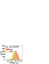
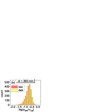
In summary, we have introduced a multiscaling formalism to study fluctuations in complex systems. We find that non-universal behavior is manifested not only in $\alpha$ exponents different from the universal values 1/2 and 1 but also in the scaling properties of the distribution functions. The $\alpha$ exponents found for the flow data of 2,200 stocks on the NYSE showed a continuous dependence on the time horizon with good quality scaling over five orders of magnitude. An additional signature of non-universal behavior is that multiscaling was found, in contrast to several other complex systems investigated in the similar fashion [6].

Acknowledgments: We thank Marcio de Menezes for useful comments and György Andor for his help with the data. JK thanks the University of Notre Dame for hospitality, and he is member of the Center for Applied Mathematics and Computational Physics, BUTE. Research at Notre Dame was supported by NSF.

References

- [1] See, e.g., http://www.cscs.umich.edu/complexity.html
- [2] Unifying Themes in Complex Systems, Ed.: Y. Bar-Yam (NECSI, 2000); Complexity Metaphors, Models, and Reality Eds.: George A. Cowan, David Pines, David Meltzer (Perseus, 1999); A.L. Barabási, Linked (Plume, 2003)
- [3] For a review see: L.P. Kadanoff, Chinese J. Phys. 29, 613 (1991)
- [4] M.A. de Menezes and A.-L. Barabási, Phys. Rev. Lett. 92, 28701 (2004)
- [5] H.E. Stanley, Introduction to Phase Transitions and Critical Phenomena (Oxford University Press, 1971)
- [6] M.A. de Menezes, A.-L. Barabási and J. Kertész, unpublished
- [7] M.A. de Menezes and A.-L. Barabási, Phys. Rev. Lett. 93, 068701 (2004)
- [8] We note that this separation does not lead to uncorrelated decomposition which can be achieved by projector technique [9].
- [9] Z. Eisler and J. Kertész (in preparation).
- [10] T. Vicsek, Fractal Growth Phenomena, World Scientific Publishing (1992)
- [11] R. N. Mantegna and H. E. Stanley (Cambridge University Press, Cambridge, 1999); J. P. Bouchaud and M. Potters, Theory of Financial Risk (Cambridge University Press, Cambridge, 2000)
- [12] P. Gopikrishnan, V. Plerou, X. Gabaix, and H. E. Stanley Phys. Rev. E 62, R4493 (2000)
- [13] The Trades and Quotes Database for 2000-2002, New York Stock Exchange, New York (2003)
- [14] We discarded all companies, that were not continuously present on the market over the -year interval and we combined different class stocks of the same company.
- [15] Calculations with shorter time horizons down to seconds reinforced this observation.
- [16] T.W. Epps, J. Amer. Stat. Assoc. 74, 291 (1979); G. Bonanno, F. Lillo and R.N. Mantegna, Quant. Finance 1, 96-104 (2001); G. Bonanno, G. Caldarelli, F. Lillo, S. Micciche, N. Vandewalle, R. N. Mantegna, Eur. Phys. J. B 38, 363 (2004);
- [17] See, e.g., L. Kullmann, J. Töyli, J. Kertész, A. Kanto, K. Kaski, Physica A 269, 98-110 (1999).
- [18] D.M. Cutler, J.M. Poterba, L.H. Summers, Journal of Portfolio Management 15, 4-12 (1989); D. Sornette and A. Helmstetter, Physica A 318, 577-591 (2003); Á.G. Zawadowski, R. Karádi, J. Kertész, Physica A 316, 403-413 (2002)