Simulation study of spatio-temporal correlations of earthquakes as a stick-slip frictional instability

Abstract

Spatio-temporal correlations of earthquakes are studied numerically on the basis of the one-dimensional spring-block (Burridge-Knopoff) model. As large events approach, the frequency of smaller events gradually increases, while, just before the mainshock, it is dramatically suppressed in a close vicinity of the epicenter of the upcoming mainshock, a phenomenon closely resembling the “Mogi doughnut”.

Earthquake is a stick-slip frictional instability of a fault driven by steady motions of tectonic platesScholzRev ; ScholzBook . While earthquakes are obviously complex phenomena, certain empirical laws have been known concerning their statistical properties, e.g., the Gutenberg-Richter (GR) law for the magnitude distribution of earthquakes, or the Omori law for the time evolution of the frequency of aftershocksScholzBook . These laws are basically of statistical nature, becoming eminent only after analyzing large number of events.

Since earthquakes could be regarded as a stick-slip frictional instability of a pre-existing fault, the statistical properties of earthquakes should be governed by the physical law of rock frictionScholzRev ; ScholzBook . One might naturally ask: How the statistical properties of earthquakes depend on the material properties characterizing earthquake faults, e.g., the elastic properties of the crust or the frictional properties of the fault, etc.

Some time ago, Carlson, Langer and collaborators performed a pioneering study of the statistical properties of earthquakes CL ; CLST ; Carlson , based on the spring-block model (Burridge-Knopoff model) BK . These authors paid particular attention to the magnitude distribution of earthquake events, and examined its dependence on the friction parameter characterizing the nonlinear stick-slip dynamics of the model. It was observed that, while smaller events persistently obeyed the GR law, i.e., staying critical or near-critical, larger events exhibited a significant deviation from the GR law, being off-critical or “characteristic”.CL ; CLST ; Carlson ; Schmittbuhl Shaw, Carlson and Langer studied the same model by examining the spatio-temporal patterns of seismic events preceding large events, observing that the seismic activity accelerates as the large event approachesShaw . Recently, many numerical works have been made for the cellular-automaton versions of the model which were introduced to mimic the original spring-block model OFC ; Hergarten ; Hainzl .

In the present Letter, we wish to further investigate the spatio-temporal correlations of earthquakes by performing extensive numerical simulations of the Burridge-Knopoff (BK) model BK . Our main goal is to clarify how the statistical properties of earthquakes depend on the friction parameter characterizing the nonlinear stick-slip dynamics. We simulate here the one-dimensional (1D) version of the BK model. It consists of a 1D array of $N$ identical blocks, which are mutually connected with the two neighboring blocks via the elastic springs of the elastic constant $k_{c}$, and are also connected to the moving plate via the springs of the elastic constant $k_{p}$. All blocks are subject to the friction force, which is the only source of the nonlinearity in the model. The time $t$ is made dimensionless here, being measured in units of the characteristic frequency $\omega=\sqrt{k_{p}/m}$ where $m$ is the mass of a block. Then, the equation of motion for the $i$-th block can be written in the dimensionless form as

$$\ddot{u}_{i}=\nu t-u_{i}+l^{2}(u_{i+1}-2u_{i}+u_{i-1})-\phi(\dot{u}_{i}),$$ (1)

where $u_{i}$ is the dimensionless displacement of the $i$-th block, $l\equiv\sqrt{k_{c}/k_{p}}$ is the dimensionless stiffness parameter, $\nu$ is the dimensionless loading rate representing the speed of the plate, and $\phi$ is the dimensionless friction force. In order for the model to exhibit a dynamical instability corresponding to an earthquake, it is essential that the friction force $\phi$ possesses a frictional weakening property, i.e., the friction should become weaker as the block slides. Here, as the form of the frictional force, we assume the form used in Ref.CLST , which represents the velocity-weakening friction force;

$$\phi(\dot{u})=\left\{\begin{array}[]{ll}(-\infty,1],&\ \ \ \ {\rm for}\ \ \dot{u}_{i}\leq 0,\\ \frac{1-\sigma}{1+2\alpha\dot{u}_{i}/(1-\sigma)},&\ \ \ \ {\rm for}\ \ \dot{u}_{i}>0,\end{array}\right.$$ (2)

where its maximum value corresponding the static friction is normalized to unity. This normalization condition $\phi(\dot{u}=0)=1$ has been utilized to set the length unit. The back-slip is inhibited by imposing an infinitely large friction for $\dot{u}_{i}<0$, i.e., $\phi(\dot{u}<0)=-\infty$.

The friction force is characterized by the two parameters, $\sigma$ and $\alpha$. The former, $\sigma$, represents an instanteous drop of the friction force at the onset of the slip, while the latter, $\alpha$, represents the rate of the friction force getting weaker on increasing the sliding velocity. Following Ref.CLST , we assume the loading rate $\nu$ to be infinitesimally small, and put $\nu=0$ during an earthquake event. Taking this limit ensures that the interval time during successive earthquake events can be measured in units of $\nu^{-1}$ irrespective of particular values of $\nu$ CLST .

Although we studied the properties of the model with varying all the parameters $\alpha$, $\sigma$ and $l$, we explicitly show here the $\alpha$-dependence only, since the parameter $\alpha$ turns out to affect the result most significantly. We mainly study the cases $\alpha=1,2$ and 3: This choice has been made because (i) Ref.CL suggested that the smaller value of $\alpha<1$ tended to cause a creeping-like behavior, and (ii) our preliminary study for larger $\alpha$ ($\alpha=5,10$) indicated that the further increase of $\alpha>3$ did not change the result qualitatively. Below, we fix $l=3$ and $\sigma=0.01$ unless otherwise stated. In order to eliminate the possible finite-size effects, the total number of blocks are taken to be large, typically $N=800$, with periodic boundary conditions. In the case of $l=3$ and $\sigma=0.01$, even the largest event in our simulations involves the number of blocks less than $N=800$. Total number of $10^{7}$ events are generated in each run.

In Fig.1 we show the magnitude distribution $R(\mu)$ of earthquake events for several values of the parameter $\alpha$, where $R(\mu){\rm d}\mu$ represents the rate of events with their magnitudes in the range [$\mu,\mu+{\rm d}\mu$]. The magnitude of an event, $\mu$, is defined as the logarithm of the moment $M_{0}$, i.e., $\mu=\ln M_{0}$ with $M_{0}=\sum_{i}\Delta u_{i}$, where $\Delta u_{i}$ is the total displacement of the $i$-th block during a given event and the sum is taken over all blocks involved in the eventCLST .

As can be seen from Fig.1, the data for $\alpha=1$ lie on a straight line fairly well, apparently satisfying the GR law. The values of the exponent $B$ describing the power-law behavior, $\propto 10^{-B}$, is estimated to be $B\simeq 0.50$. The data for larger $\alpha$, i.e., for $\alpha=2$ and 3, deviate from the GR law at larger magnitudes, exhibiting a clear peak structure, while the power-law feature still remains for smaller magnitudes. These features of the magnitude distribution are consistent with the earlier observation of Carlson and Langer CL ; CLST . The observed peak structure gives us a criterion to distinguish large and small events. Below, we regard events with their magnitudes $\mu$ greater than $\mu_{c}=3$ as large events, $\mu_{c}=3$ being close to the peak position of the magnitude distribution of Fig.1. In an earthquake with $\mu=3$, the mean number of moving blocks are about 76 ($\alpha=1$) and 60 ($\alpha=2,3$).

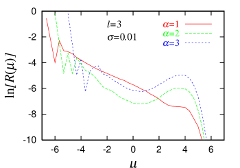
Figure 1: Magnitude distribution of earthquake events for various values of $\alpha$.

One question of general interest is how large earthquakes repeat in time, do they occur near periodically or irregularly? One may ask this question either locally, i.e., for a given finite area on the fault, or globally, i.e., for an entire fault system. In Fig.2, we show the distribution of the recurrence time $T$ of large earthquakes with $\mu_{c}=3$, measured either locally (a), or globally (b). In the insets, the same data including the tail part are re-plotted on a semi-logarithmic scale. In defining the recurrence time locally, the subsequent large event is counted when a large event occurs with its epicenter in the region within 30 blocks from the epicenter of the previous large event. The mean recurrence time $\bar{T}$ is then estimated to be $\bar{T}\nu=1.47$, 1.12, and 1.13 for $\alpha=1$, 2 and 3, respectively.

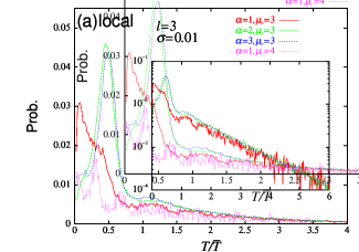
Figure 2: The recurrence-time distribution of large events with their magnitudes greater than $\mu_{c}=3$ or 4 for various values of $\alpha$, the local one (a) and the global one (b). The recurrence time $T$ is normalized by its mean $\bar{T}$. The total number of blocks is $N=800$. Even the largest event involves the number of blocks less than $N=800$. The insets represent the semi-logarithmic plots including the tail part of the distribution.

The local recurrence-time distribution shown in Fig.2(a) has the following two noticeable features. (i) The tail of the distribution is exponential at longer $T\buildrel\textstyle>\over{{}_{\sim}}\bar{T}$ for all values of $\alpha$. Such an exponential tail of the distribution has also been reported for real faultsCorral . (ii) The form of the distribution at shorter $T\buildrel\textstyle<\over{{}_{\sim}}\bar{T}$ is non-exponential, and largely differs between for $\alpha=1$ and for $\alpha=2$ and 3. For $\alpha=2$ and 3, the distribution has an eminent peak at around $\bar{T}\nu\simeq 0.5$, not far from the mean recurrence time. Here we regard such an appearance of a characteristic recurrence time as a signature of the near-periodic recurrence of large events. Indeed, such a near-periodic recurrence of large events was reported for several real faults ScholzBook ; NB .

For $\alpha=1$, by contrast, the peak located close to the mean $\bar{T}$ is hardly discernible. Instead, the distribution has a pronounced peak at a shorter time $\bar{T}\nu\simeq 0.10$, just after the previous large event. In other words, large events for $\alpha=1$ tend to occur as “twins”. This has also been confirmed by our analysis of the time record of large events. Closer examination of individual event has revealed that a large event for $\alpha=1$ often occurs as a “unilateral earthquake” where the rupture propagates only in one direction, hardly propagating in the other direction. In other words, for $\alpha=1$, the epicenter of large events tend to be located near the edge of the rupture zone. This can be confirmed more quantitatively by calculating the “eccentricity” of the epicenter $\epsilon=R^{*}/\bar{R}$, which is defined by the ratio of the mean distance between the epicenter and the center of mass of the rupture zone, $R^{*}$, to the mean radius of the rupture zone, $\bar{R}$. Then, we have found $\epsilon=0.88$, 0.52 and 0.53 for the cases $\alpha=1$, 2 and 3, respectively. The occurrence of unilateral earthquakes for smaller $\alpha$ may be understandable if one notes that the relative weakness of the stick-slip instability prevents the initiated rupture from propagating far into both directions. When a large earthquake occurs in the form of such a unilateral earthquake, further loading due to the plate motion tends to trigger the subsequent large event in the opposite direction, causing a twin-like event. This naturally explains the small-$T$ peak observed in Fig.2(a) for $\alpha=1$.

We note, however, that even in the case of $\alpha=1$ the periodic character of events becomes appreciable when one looks at very large events. In Fig.2(a), the recurrence-time distribution for very large events, characterized by still larger magnitude threshold $\mu_{c}=4$, is shown for the case of $\alpha=1$. Interestingly, the distribution in this case has two distinct peaks, one corresponds to the twin-like event and the other corresponds to the near-periodic event. Hence, even in the case of $\alpha=1$ where the critical features are apparently dominant, features of characteristic earthquake becomes increasingly eminent when one looks at very large events.

The global recurrence-time distribution, i.e., the one for an entire fault system with $N=800$, takes a different form from the local one, as can be seen from Fig.2(b). The peak structure seen in the local distribution no longer exists here. Furthermore, the form of the distribution tail at larger $T$ is no longer a simple exponential, faster than exponential: See a curvature of the data in the inset of Fig.2(b).

Carlson Carlson and Schmittbuhl et al Schmittbuhl reported a periodic behavior of large events by studying the global distribution function of the model of smaller size $N=100$ with $l=10$. We have found that, for such a large value of $l$, even an $N=800$ system behaves almost as a rigid body and exhibits a near-periodic behavior, where the larger events often penetrates the entire $N=800$ system. We note that, generally speaking, whether the recurrence-time distribution exhibits a periodic peak depends on the length scale of measurements as well as on the values of the parameters $\alpha$ and $l$. Such scale-dependent features of the recurrence-time distribution of the BK model is in apparent contrast with the scale-invariant features of the recurrence-time distributions recently reported for some of real faults Bak ; Corral .

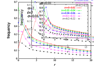
Figure 3: Event frequency preceding the large event with $\mu>\mu_{c}=3$ plotted versus $r$, the distance from the epicenter of the upcoming mainshock, for $\alpha=2$ and for several time periods before the mainshock. The inset represents the weighted event frequency with the weight of the event size (the number of blocks): See the text for details.

In order to “predict” the large event, one usually probes the precursory phenomena associated with the large event. Fig.3 represents the space-time correlation function between the large events and the preceding events of arbitrary size (dominated in number by smaller events): It represents the conditional probability that, provided that a large event with $\mu>\mu_{c}=3$ occurs at a time $t_{0}$ and at a spatial point $r_{0}$, an event of arbitrary size occurs at a time $t_{0}-t$ and at a spatial point $r_{0}\pm r$. The calculated correlation functions for the case of $\alpha=2$ are shown as a function of $r$ for several time periods before the mainshock.

As can be seen from Fig.3, preceding the large event, there is a clear tendency of the frequency of smaller events to be enhanced at and around the epicenter of the upcoming mainshock Shaw . For small enough $t$, such a cluster of smaller events correlated with the large event may be regarded as foreshocks. An interesting feature revealed here is that, as the mainshock becomes imminent, the frequency of smaller events is suppressed in a close vicinity of the epicenter of the upcoming mainshock, though it continues to be enhanced in the surroundings. For real earthquake faults, such a quiescence phenomenon has been discussed as the “Mogi doughnut”Mogi ; ScholzBook .

One may wonder if our way of measuring the seismicity by simply counting the number of events may over-weigh the contribution of the single-block events which are by far the most frequent events. In order to examine this point, we show in the inset of Fig.3 the weighted correlation function in which the frequency of small events is counted with the weight proportional to its size (the number of blocks involved in that event). To eliminate the contribution of the large event, we count here only the small events with its size less than 10 blocks. As can be seen from the inset, essentially the same quiescence phenomena as shown in the main panel have been observed, suggesting that the quiescence observed here is a robust property of the model. Simulations done with varying the $\alpha$-values have revealed that such a Mogi-doughnut quiescence tends to to be enhanced with increasing $\alpha$.

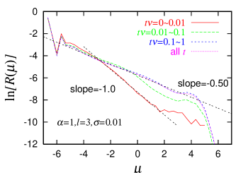
Figure 4: Local magnitude distribution preceding the mainshock with $\mu>\mu_{c}=3$, for $\alpha=1$ and for several time periods before the mainshock.

The present observation contrasts with the earlier work of Carlson, who claimed that the 1D BK model did not exhibit such a Mogi-doughnut quiescence Carlson . We note that the quiescence observed here occurs only in a close vicinity of the epicenter of the mainshock, within one or two blocks from the epicenter, and only at a time close to the mainshock, $t\nu\buildrel\textstyle<\over{{}_{\sim}}0.02$. Thus, the better statistics and the better resolution of the present simulation have been essential to uncover this effect.

As an other signature of the precursory phenomena, we show in Fig.4 the “time-resolved” local magnitude distribution for the case of $\alpha=1$ for several time periods before the large event. Only the events with their epicenters within 30 blocks from the upcoming mainshock is counted here. As can be seen from the figure, as the mainshock approaches, the form of the magnitude distribution changes significantly. In particular, the apparent $B$-value describing the power-law regime tends to increase as the mainshock approaches, from the time-averaged mean value $\simeq 0.50$ to the value $\simeq 1.0$ just before the mainshock: It is almost doubled. Interestingly, a similar increase of the apparent $B$-value preceding the mainshock was reported for real faults Smith . For the case of larger $\alpha$, $\alpha=2$ and 3, the change of the $B$-value preceding the mainshock is still appreciable (the data not shown here), though in a less pronounced manner. While the observed change in the magnitude distribution might simply be understood as caused by a supression of larger events prior to the mainshock, we emphasize it is a real observable effect if one monitors the time change of the local magnitude distribution.

In summary, we studied the spatio-temporal correlations of the 1D BK model of earthquakes. Periodic feature of large events is eminent when the friction force exhibits a strong frictional instability, whereas, when the friction force exhibits a weak frictional instability, large events often occur as twin and/or unilateral events. Preceding the mainshock, the frequency of smaller events is gradually enhanced, whereas, just before the mainshock, it is dramatically suppressed in a close vicinity of the epicenter of the upcoming mainshock (the Mogi doughnut). Under certain conditions, preceding the mainshock, the apparent $B$-value of the magnitude distribution increases significantly. These properties may be used in predicting the time and the position of the upcoming large event.

References

- (1) C.H. Scholz, Nature 391, 3411 (1998).
- (2) C.H. Scholz, The Mechanics of Earthquakes and Faulting (Canbridge Univ. Press, 1990).
- (3) J.M. Carlson and J.S. Langer, Phys. Rev. Lett. 62, 2632 (1989); Phys. Rev. A40, 6470 (1989).
- (4) J.M. Carlson, J.S. Langer, B.E. Shaw and C. Tang, Phys. Rev. A44, 884 (1991).
- (5) J.M. Carlson, J. Geophys. Res. 96, 4255 (1991).
- (6) R. Burridge and L. Knopoff, Bull. Seismol. Soc. Am. 57 (1967) 3411.
- (7) J. Schmittbuhl, J.-P. Vilotte and S. Roux, J. Geophys. Res. 101, 27741 (1996).
- (8) B.E. Shaw, J.M. Carlson and J.S. Langer, J. Geophys. Res. 97, 479 (1992).
- (9) Z. Olami, H.J. Feder and K. Christensen, Phys. Rev, Lett. 68, 1244 (1992).
- (10) S. Hergarten and H. Neugebauer, Phys. Rev. Lett. 88, 238501 (2002).
- (11) S. Hainzl, G. Zöller and J. Kurths, J. Geophys. Res. 104, 7243 (1999); Geophys. Res. Lett. 27, 597 (2000).
- (12) A. Corral, Phys. Rev. Lett. 92, 108501 (2004).
- (13) S.P. Nishenko and R. Buland, Bull. Seismol. Soc. Am. 77, 1382 (1987).
- (14) P. Bak, K. Christensen, L. Danon and T. Scanlon, Phys. Rev. Lett. 88, 178501 (2002).
- (15) K. Mogi, Bull. Earthquake Res. Inst. Univ. Tokyo 47, 395 (1969); Pure Appl. Geophys. 117, 1172 (1979).
- (16) W.D. Smith, Nature 289, 136 (1981).