Statistics of Weighted Tree-Like Networks

Abstract

We study the statistics of growing networks with a tree topology in which each link carries a weight $(k_{i}k_{j})^{\theta}$, where $k_{i}$ and $k_{j}$ are the node degrees at the endpoints of link $ij$. Network growth is governed by preferential attachment in which a newly-added node attaches to a node of degree $k$ with rate $A_{k}=k+\lambda$. For general values of $\theta$ and $\lambda$, we compute the total weight of a network as a function of the number of nodes $N$ and the distribution of link weights. Generically, the total weight grows as $N$ for $\lambda>\theta-1$, and super-linearly otherwise. The link weight distribution is predicted to have a power law form that is modified by a logarithmic correction for the case $\lambda=0$. We also determine the node strength, defined as the sum of the weights of the links that attach to the node, as function of $k$. Using known results for degree correlations, we deduce the scaling of the node strength on $k$ and $N$.

I Introduction

The recent interest in networks stems from the discovery that the node degree distribution can have a power law form. Here the node degree is defined as the number of links that are connected to this node. It is now well documented that a wide variety of natural and man-made networks have power-law degree distributions net-rev .

In most previous studies, it has been implicitly assumed that the quality of each link is identical. However, there are many examples of networks in which the weight of each link can be distinct. For example, in scientific collaborations, co-authors can have a variable number of joint publications. Thus in the associated co-authorship network, a link between two individuals represents the collaboration strength, such as the number of jointly-authored publications New ; B .

Transportation networks represent another situation where the weight of each link is variable. In the specific example of airline route networks, links between two airports represent the passenger capacity on this route air . It has been found that the weight of the link (defined as the number of available seats on flights between the two airports connected by the link) is well-approximated by the products of the endpoint degrees raised to a power orsay . A related line of research focuses on general properties of flows in heterogeneous networks F1 ; F2 .

A third example where link weights are connected to network topology occurs in the metabolic network of the bacterium E. coli. Here a link between two metabolic substrates represents an enzymatic reaction, and the weight of a link (defined as the metabolic flux rate) displays the same functional dependence on the endpoint degrees as that of the world airline network macdonald .

There has also been much very recent work on various aspects of weighted networks including characterizing paths on these networks NR , structural properties hui ; New2 , and the application to weighted networks to diverse physical systems, such as earthquakes maya and to synchronization phenomena jurgen .

In this work, we characterize basic properties of growing networks in which the links possess variable weights BBV . We consider the generic situation in which network growth is governed only by the node degrees, so that the link weights are passive subsidiary variables. (The comlementary situation in which the link weights determine network growth has also been analyzed, see, e.g., Refs. macdonald ; NR ; hui ; BBV ; AK ). We define the weight $w_{ij}$ of a link between nodes $i$ and $j$ in the network to be the product of endpoint node degrees; that is, $w_{ij}=k_{i}k_{j}$. More generally, we study the general case where the link weight has the following dependence on the endpoint degrees:

$$w_{ij}=(k_{i}k_{j})^{\theta}.$$ (1)

We show that this weighted network has a surprising dependence of the total weight on the system size and an unusual scaling for the distribution of link weights. Many of the new results that we obtain follow naturally from previous work on the degree correlations in growing networks KR .

For the network growth mechanism, we employ preferential attachment, in which a new node links to previous nodes with an attachment rate $A_{k}$ that depends only on the degree of the “target” node BA . For simplicity, we consider the situation where the newly-introduced node connects to a single target. Because of this topological restriction, the resulting network is a tree, a feature that turns out to simplify our analysis. To complete the description of the system, we need to specify the attachment rate $A_{k}$. We will consider the Simon model simon , where $A_{k}=k+\lambda$, with $\lambda>-1$ but otherwise arbitrary. For this growth mechanism the degree distribution has a power law tail $\propto k^{-3-\lambda}$.

In the next section we compute the total network weight $W(N)$, defined as the sum of the link weights $w_{ij}$, as a function of the total number of nodes $N$. The distribution of link weights is investigated in Sec. III, and the node strength, defined as the sum of the weights of all the links that attach to the node, is studied in Sec. IV. We first focus on the case of the strictly linear attachment rate where $A_{k}=k$ and then outline corresponding results for the more general case of $A_{k}=k+\lambda$ with $\lambda>-1$ but otherwise arbitrary. Numerical simulation results and comparison to our analytic predictions are given in Sec. V.

II Total Network Weight

We denote by $N_{k,l}(N)$ the number of nodes of degree $k$ that attach to an ancestor node of degree $l$. This degree correlation function is well-defined only for growth processes in which each node attaches to exactly one previous node, so that the ancestor of each node is unique. Notice that the correlation function $N_{k,l}$ is not symmetric with respect to the end nodes. For graphs that are built sequentially by preferential attachment, we are interested in the total weight of the network, defined by

$$W(N)=\sum_{k,l}kl\,N_{k,l}(N)\,.$$ (2)

That is, we first consider the case of $\theta=1$ in Eq. (1).

For growth processes in which the attachment rate $A_{k}$ does not grow faster than linearly with $k$, the correlation function $N_{k,l}(N)$ grows linearly with the total number of nodes $N$ (see KR , and also rev for a brief review). That is, $N_{k,l}(N)=Nn_{k,l}$ for large $N$. The explicit form of the distribution $n_{kl}$ for the simplest case of the Barabási-Albert (BA) model ($\lambda=0$) is KR

$$n_{k,l} = \frac{4(l-1)}{k(k+1)(k+l)(k+l+1)(k+l+2)}$$ (3)

$$+ \frac{12(l-1)}{k(k+l-1)(k+l)(k+l+1)(k+l+2)}\,.$$

Since $W(N)=N\sum kl\,n_{k,l}$, one might naively anticipate that the total weight will scale linearly with $N$. This expectation is erroneous because the infinite sum $\sum kl\,n_{k,l}$ formally diverges, leading to an additional $N$ dependence in $W(N)$.

To compute $\sum kl\,n_{k,l}$ we write $m=k+l$ and recast the sum as

$$\sum_{k,l}kl\,n_{k,l} = \sum_{m\geq 2}\frac{4}{m(m+1)(m+2)}\sum_{l=2}^{m-1}\frac{l(l-1)}{m+1-l}$$

$$+ \sum_{m\geq 2}\frac{12}{(m-1)m(m+1)(m+2)}\sum_{l=2}^{m-1}l(l-1).$$

For large $m$, the internal sums behave as

$$\sum_{l=2}^{m-1}\frac{l(l-1)}{m+1-l} = m^{2}\ln m+{\cal O}(m^{2}),$$

$$\sum_{l=2}^{m-1}l(l-1) = \frac{1}{3}\,m^{3}+{\cal O}(m^{2}).$$

Thus the asymptotically dominant part of the sum is

$$\sum_{k,l}kl\,n_{k,l}\sim\sum_{m\geq 2}\frac{4\,\ln m}{m}+\sum_{m\geq 2}{\cal O}(m^{-1})$$ (4)

To evaluate these sums explicitly, we need to impose a cutoff in the upper limit. For the case $\lambda=0$, we therefore use the fact that the maximal degree $k_{\rm max}$ scales as $N^{1/2}$ BA ; KR-finite . This result is easy to derive by utilizing $N_{k}\sim 4Nk^{-3}$ and estimating the maximal degree from the extremal criterion that in a network of $N$ nodes, there will be a single node whose degree in the range $(k_{\rm max},\infty)$. This criterion corresponds to the condition $\sum_{k\geq k_{\rm max}}N_{k}=1$. Thus we cut off the sums in (4) at $m_{\rm max}\sim(2N)^{1/2}$ to give

$$\sum_{k,l}kl\,n_{k,l}=\frac{1}{2}\,(\ln N)^{2}+{\cal O}(\ln N).$$ (5)

Since the leading sum in (4) diverges logarithmically, the mere knowledge of the scale of the cutoff is sufficient to determine the exact asymptotics. With this result for the internal sums, we thereby find, from (2),

$$W(N)=\frac{1}{2}\,\,N(\ln N)^{2}+{\cal O}(N\ln N).$$ (6)

A similar computation for the Simon model (where $A_{k}=k+\lambda$) with arbitrary $\lambda$ is difficult to perform exactly because the expression for $n_{k,l}$ is an infinite series KR rather than a rational function as in Eq. (3). However, the dominant contribution to the sum $\sum_{k,l}kl\,n_{k,l}$ is concentrated in the region $1\ll k\ll l$, where $n_{k,l}$ admits the simple asymptotic form KR

$$n_{k,l}\sim k^{-2}l^{-2-\lambda}\,.$$ (7)

Therefore

$$\sum_{k,l}kl\,n_{k,l}\sim\sum l^{-1-\lambda}\sum_{k\ll l}k^{-1}\sim\sum l^{-1-\lambda}\,\ln l.$$ (8)

For $\lambda>0$ the sum converges, while for $\lambda\leq 0$ the sum formally diverges and we must again determine an upper cutoff. Applying the previously-mentioned extremal argument for the maximal node degree for general values of $\lambda$, we now find $k_{\rm max}\propto N^{1/(2+\lambda)}$ KR-finite . Thus we conclude that the last sum in Eq. (8) scales as $N^{-\lambda/(2+\lambda)}\,\ln N$ for $-1<\lambda<0$. In summary,

$$W(N)\propto\begin{cases}N&\lambda>0;\cr N\,(\ln N)^{2}&\lambda=0;\cr N^{2/(2+\lambda)}\ln N&\lambda<0.\end{cases}$$ (9)

Consider now the situation where link weight depends on its endpoint degrees according to Eq. (1). We treat only the case $\theta<1$ because this regime corresponds to real networks orsay ; macdonald . Using the asymptotic behavior for $n_{k,l}$ given in Eq. (7), we then have

$$\sum_{k,l}(kl)^{\theta}\,n_{k,l}\sim\sum l^{-2-\lambda+\theta},$$

which converges for $\lambda>\theta-1$ and diverges otherwise. Thus in the range $\theta$ strictly less than 1, the total weight of the network scales according to

$$W(N)\sim\begin{cases}N&\lambda>\theta-1;\cr N\ln N&\lambda=\theta-1;\cr N^{(1+\theta)/(2+\lambda)}&\lambda<\theta-1.\end{cases}$$ (10)

III Link Weight Distribution

In this section, we consider exclusively the case of $\theta=1$. We define the link weight distribution $\Pi(w)$ as the fraction of links whose weight equals $w$. That is,

$$\Pi(w)=\sum_{\stackrel{{\scriptstyle k,l}}{{kl=w}}}\,n_{k,l}$$ (11)

This natural definition leads to erratic behavior in the distribution, as the arithmetic nature of $w$ plays a significant role. If $w$ is prime, then the only possible degrees of the end nodes are $1$ and $w$, while if $w$ has many divisors, there are more possibilities for the degrees of the end nodes. Thus in addition to an expected global smooth dependence of $\Pi(w)$ on $w$, there will be superimposed fluctuations related to the divisibility of $w$. These fluctuations will disappear if we average $\Pi(w)$ over a range much less than $w$ and much larger than the average distance between successive primes (which grows as $\ln w$ Hardy ). This suggests that we also consider a smoothed distribution ${\mathcal{P}}(w)$ defined by

$$\mathcal{P}(w)=w^{-a}\sum_{w\leq kl\leq w+w^{a}}\,n_{k,l},$$ (12)

with $a$ in the range $0<a<1$. For sufficiently large $w$ this smoothed distribution should be monotonic and independent of $a$.

To determine the behavior of the link weight distribution for $w\gg 1$, we again start with the case of the BA model where $\lambda=0$. Using (3) and writing $l=w/k$ we obtain, for large $w$,

$$\Pi(w)\to\sum_{k|w}\left[\frac{4w}{(k^{2}+w)^{3}}+\frac{12wk^{2}}{(k^{2}+w)^{4}}\right].$$ (13)

The notation $k|w$ means that this sum runs over all values of $k$ that are divisors of $w$. For large $w$, the asymptotic behavior of the summand scales as $w^{-2}$ times the average number of divisors of $w$. Using the celebrated Dirichlet formula (see e.g., Hardy ), the total number of divisors of all integers from 1 to $w$ is

$$\sum_{x=1}^{w}d(x)=w\ln w+(2\gamma-1)w+\ldots,$$

where $d(x)$ is the number of divisors of the integer $x$ and $\gamma\cong 0.577215$ is the Euler-Mascheroni constant. Thus the average number of divisors of $w$ grows logarithmically with $w$; more precisely, by differentiating the above formula with respect to $w$, we have $\langle d(w)\rangle\to\ln w+2\gamma$. Thus the tail of the weight distribution is

$${\mathcal{P}}(w)\sim w^{-2}\,\ln w\qquad{\rm as}\quad w\gg 1.$$ (14)

Consider now the general case of arbitrary $\lambda$ (but with the necessary constraint $\lambda>-1$ to ensure a finite average degree). In this case, we have to combine two separate contributions to determine the link weight distribution. First, using $kl=w$, we re-write Eq. (7) as

$$n_{k,l}\sim k^{\lambda}\,w^{-2-\lambda}.$$ (15)

This asymptotic behavior holds for $k<l$, so it can be used to estimate the part of the sum in Eq. (11) that runs over the divisors $k|w$ such that $k<\sqrt{w}$. The corresponding contribution to the weight distribution is therefore

$${\mathcal{P}}_{<}(w)\sim w^{-2-\lambda}\sigma_{\lambda}(\sqrt{w}),$$ (16)

where $\sigma_{\lambda}(n)$ is the generalized divisor function of $n$ defined as

$$\sigma_{\lambda}(n)=\sum_{f|n}f^{\lambda}\,,$$ (17)

where the sum runs over all divisors $f$ of the integer $n$. This generalized divisor function exhibits, on average, a power-law growth in $n$ for $\lambda>0$, $\sigma_{\lambda}(n)\sim n^{\lambda}$, and approaches a constant for $\lambda<0$ Sch . As a result, the asymptotic behavior of ${\mathcal{P}}_{<}(w)$ undergoes a qualitative change when $\lambda$ passes through zero. Using the result for the generalized divisor function in Eq. (16), we find, for the contribution to the link weight distribution from divisors of $w$ that are smaller than $\sqrt{w}$:

$${\mathcal{P}}_{<}(w)\sim\begin{cases}w^{-2-\lambda/2}&\lambda>0,\cr w^{-2-\lambda}&\lambda<0.\end{cases}$$ (18)

A second contribution to the weight distribution arises from the range $k>l$. (For the following arguments we use the smoothed weight distribution of Eq. (12). Correspondingly, the generalized divisor function $\sigma_{\lambda}(n)$ should also be averaged in the same way as that for the weight distribution in Eq. (12).)  In this case, the asymptotic behavior of the distribution $n_{k,l}$ is KR

$$n_{k,l}\sim l\,^{6+3\lambda}\,w^{-5-2\lambda}$$ (19)

We use this asymptotics to estimate the part of the sum in Eq. (11) that runs over the divisors $k|w$ such that $k>\sqrt{w}$, or equivalently over divisors $l|w$ such that $l<\sqrt{w}$. The corresponding contribution to the weight distribution is

$${\mathcal{P}}_{>}(w)\sim w^{-5-2\lambda}\sigma_{6+3\lambda}(\sqrt{w})$$ (20)

Since $6+3\lambda>0$ (in fact, the stronger inequality $6+3\lambda>3$ holds), the generalized divisor function behaves as $\sigma_{6+3\lambda}(\sqrt{w})\sim w^{3+3\lambda/2}$. Thus

$${\mathcal{P}}_{>}(w)\sim w^{-2-\lambda/2}.$$ (21)

We therefore find that the large-$w$ tail of the complete weight distribution ${\mathcal{P}}(w)={\mathcal{P}}_{<}(w)+{\mathcal{P}}_{>}(w)$ is dominated by ${\mathcal{P}}_{<}(w)$. Thus summarizing our results, the link weight distribution is

$${\mathcal{P}}(w)\sim\begin{cases}w^{-2-\lambda/2}&\lambda>0;\cr w^{-2}\,\ln w&\lambda=0;\cr w^{-2-\lambda}&\lambda<0.\end{cases}$$ (22)

The average weight per link $\langle w\rangle=\int dw\,w\,\Pi(w)$ should be equal $W(N)/N$. In computing $\langle w\rangle$ using Eq. (22), we find agreement with Eq. (9) only for $\lambda\geq 0$. The reason for the disagreement in the range $-1<\lambda<0$ is unclear. Part of difficulty may lie in the fact that the link weight distribution exhibits an anomalous feature that is not simply a power-law behavior (see Sec. V).

IV Node Strength

Many real networks display a significant correlation between the degrees of adjacent nodes. There are examples where there is a bias for nodes to be connected to other nodes with either similar (assortative) or different (disassortative) degree newman . This tendency to select nodes with a consonant property is often expressed as a Pearson correlation coefficient of the network. For networks where the weights are correlated with the topology, we investigate the effects of correlations by studying the node strength defined as orsay

$$s_{i}~{}=~{}\sum_{\langle ji\rangle}w_{ij},$$ (23)

where the sum runs over all nodes $j$ that are linked to node $i$. Let us first consider the simplest link weight function where $w_{ij}$ is just the product of the endpoint node degrees. Then the strength $s(k)$ of a node of degree $k$ is simply $k$ times the sum of the degrees of the neighboring nodes. Since there are $k$ neighbors, $s(k)$ is then $k^{2}$ times the average degree of the neighboring nodes if we ignore correlations between the degrees of neighboring nodes. Now the average node degree equals twice the number of links divided by the number of nodes; this simply equals 2 for a network with a tree topology. Hence the node strength $s(k)$ scales as

$$s(k)\sim k^{2}\,.$$ (24)

Because node degrees are actually correlated, we now investigate their influence on the simple prediction of Eq. (24). To include the effect of node correlations on the behavior of the node strength $s(k)$, we start by splitting the contributions to $s(k)$ into two parts: one from incoming links and another from the outgoing link. This gives

$$s(k)=s_{\rm in}(k)+s_{\rm out}(k)=(k-1)k\,\langle j_{k}\rangle_{\rm in}+k\,\langle l_{k}\rangle_{\rm out}\,.$$ (25)

The first term accounts for the fact that there are $k-1$ incoming links, each of which has weight $k\,j_{k}$, where $j_{k}$ denotes the degree of a daughter node when the initial node has degree $k$. Similarly, the second term accounts for the single ancestor node with degree $l_{k}$. We now consider these two contributions to $s(k)$ separately.

For the contribution due to the ancestor node, we use the fact that its average degree $\langle l_{k}\rangle_{\rm out}$ is given by

$$\langle l_{k}\rangle_{\rm out}=\frac{\sum_{l\geq 1}l\,n_{k,l}}{\sum_{l\geq 1}n_{k,l}}.$$ (26)

The normalization factor is just the degree distribution

$$\sum_{l\geq 1}n_{k,l}=n_{k}=\frac{4}{k(k+1)(k+2)}.$$

Using this, together with Eq. (3), we obtain (again using the shorthand notation $m=k+l$)

$$\langle l_{k}\rangle_{\rm out}=(k+2)\sum_{l\geq 1}\frac{l(l-1)}{m(m+1)(m+2)}$$

$$+3(k+1)(k+2)\sum_{l\geq 1}\frac{l(l-1)}{(m-1)m(m+1)(m+2)}\,.$$

The first sum on the right-hand side is logarithmically divergent. Using the fact the upper cutoff is $\sqrt{N}$ and replacing the sum by an integral, we find that for $k\gg 1$ the first sum is asymptotic to $\ln\sqrt{N}-\ln k$. Similarly we find that the second sum is asymptotic to ${1}/({3k})$. Therefore

$$s_{\rm out}(k)=k\,\langle l_{k}\rangle_{\rm out}\to k^{2}\left(\ln\sqrt{N}-\ln k\right)\,.$$ (27)

For the contribution to $s(k)$ from the daughter nodes, we need the average degree of these nodes. This is given by

$$\langle j_{k}\rangle_{\rm in}=\frac{\sum_{j\geq 1}j\,n_{j,k}}{\sum_{j\geq 1}n_{j,k}}\,.$$ (28)

The denominator is found from

$$\sum_{j\geq 1}n_{j,k}=(k-1)\,n_{k}=\frac{4\,(k-1)}{k(k+1)(k+2)}.$$

This equality is somewhat subtle. A node of degree $k$ has $k-1$ incoming daughter nodes. If we sum the two-point correlations functions for all these daughter nodes, we overcount the number of nodes of degree $k$ by exactly the factor $k-1$. The numerator can be computed straightforwardly but tediously by following similar steps to those preceding Eq. (27) to evaluate the sums. The resulting asymptotic behavior has the simple form $4\,k^{-2}\,\ln k$. Thus we have

$$s_{\rm in}(k)=(k-1)k\,\langle j_{k}\rangle_{\rm in}\to k^{2}\ln k$$ (29)

Consequently, for $k\gg 1$ the node strength scales

$$s(k)\to\frac{1}{2}\,k^{2}\ln N\,.$$ (30)

A note of warning is in order. The above computation of the contribution of the outgoing link to the node strength is exact — both $s_{\rm out}(k)=k\,\langle l_{k}\rangle_{\rm out}$ and Eq. (26) are manifestly correct, and therefore the knowledge of $n_{k,l}$ suffices to determine $s_{\rm out}(k)$. On the other hand, an exact calculation of the contribution of incoming links requires knowing the many-body correlation function $n(j_{1},\ldots,j_{k-1})$. This quantity gives the fraction of nodes of degree $k$ whose daughter nodes have degrees $j_{1},\ldots,j_{k-1}$. This exact contribution has the form

$$s_{\rm in}(k) = k\,\langle j_{1}+\ldots+j_{k-1}\rangle_{\rm in}\,,$$

$$= k\,\frac{\sum_{j_{1},\ldots,j_{k-1}}(j_{1}+\ldots+j_{k-1})\,n(j_{1},\ldots,j_{k-1})}{\sum_{j_{1},\ldots,j_{k-1}}n(j_{1},\ldots,j_{k-1})}\,.$$

Unfortunately, we do not know $n(j_{1},\ldots,j_{k-1})$, so we cannot compute $s_{\rm in}(k)$ exactly. Equations (25) and (28), which involve only the known degree correlation $n_{k,l}$, are based on the assumption that the degrees of the daughter nodes are uncorrelated. Although the correlation between the degrees of daughter nodes is certainly smaller than the degree correlation between the daughter and mother nodes, it is not clear that we can ignore these correlations.

Consider now the general linear attachment kernel $A_{k}=k+\lambda$ with $\lambda>-1$ and choose the weight function $w_{ij}=(k_{i}k_{j})^{\theta}$ with $\theta<1$. We now compute the contribution of the outgoing link to the node strength. We have

$$s_{\rm out}(k)=\frac{k^{\theta}}{n_{k}}\,\sum_{l\geq 1}l^{\theta}\,n_{k,l}$$ (31)

In performing this sum, we use the asymptotics $n_{k}\sim k^{-3-\lambda}$ for $k\gg 1$ and the results of KR for the asymptotics of $n_{k,l}$,

$$n_{k,l} \sim k^{-5-2\lambda}\,l^{1+\lambda}\qquad{\rm for}\quad 1\ll l\ll k\,$$

$$n_{k,l} \sim k^{-2}l^{-2-\lambda}\qquad\quad{\rm for}\quad 1\ll k\ll l\,.$$

We estimate the formally diverging sums by using the cutoff $N^{1/(2+\lambda)}$. We thus find

$$s_{\rm out}(k)\sim\begin{cases}k^{2\theta}&\lambda>\theta-1;\cr k^{2+2\lambda}(\ln N^{1/(2+\lambda)}-\ln k)&\lambda=\theta-1;\cr k^{1+\lambda+\theta}\,N^{(\theta-1-\lambda)/(2+\lambda)}-k^{2\theta}&\lambda<\theta-1.\end{cases}$$

Finally, we specialize this prediction to the simplest weight function $w_{ij}=k_{i}k_{j}$, as we report simulation results only in this particular case in the next section:

$$s_{\rm out}(k)\sim\begin{cases}k^{2}&\lambda>0;\cr k^{2}(\ln\sqrt{N}-\ln k)&\lambda=0;\cr k^{2+\lambda}\,N^{-\lambda/(2+\lambda)}-k^{2}&\lambda<0.\end{cases}$$ (32)

V Simulation Results

We now present numerical results for the total weight of a network and the underlying weight and strength distributions. To generate the network, we use the redirection method, as discussed in Ref. KR . In this approach, we attach a new node to a randomly-selected target node with probability $1-r$ and attach to the direct ancestor of this target with probability $r$. This method is both extremely simple, because the target node is randomly selected, and efficient, since the time to build a network of $N$ nodes scales linearly with $N$.

As discussed in Ref. KR , this redirection rule is equivalent to a network in which the attachment rate $A_{k}$ to a node of degree $k$ equals $k+\lambda$, with $\lambda=\frac{1}{r}-2$. The attachment rate $k+\lambda$ then leads to a degree distribution $n_{k}\sim k^{-\nu}$, with $\nu=3+\lambda$ KR . Thus by implementing redirection, we can generate scale-free networks with degree distribution exponent anywhere in the range $(2,\infty)$. As a parenthetical technical point, each node in the initial network must have a unique ancestor to ensure that redirection weights each network realization correctly KR-finite . In our simulations, we chose the starting network to be a triangle in which each node points cyclically to its nearest neighbor. This detail about initial condition does not affect the asymptotic form of the degree distribution.

Figure 1: Average network weight $W(N)$ as a function of $N$ for the representative cases $\lambda=100,1,0$, and $-2/3$, $(\circ,+,\Delta,\nabla)$, respectively.

Figure 2: Same as in Fig. 1, except that the data for $\lambda=0$ and $\lambda<0$ has been divided by $(\ln N)^{2}$ and by $\ln N$, respectively. The solid lines are best fits to the data for $N>4\times 10^{5}$. The slopes of these lines are 0.990, 0.988, 0.969, and $1.489$ for $\lambda=100,1,0$, and $-2/3$, respectively.

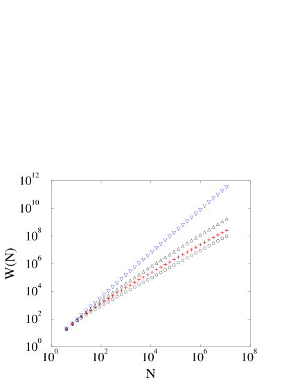
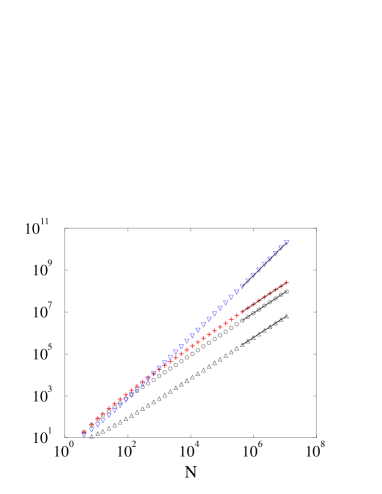
Figure 1 shows the average network weight as a function of the total number of nodes $N$. These results are based on 100 realizations of the network that each contain up to $N_{\rm max}=(1.5)^{40}\approx 1.1\times 10^{7}$ nodes. On a double logarithmic scale, the data for $W(N)$ versus $N$ is quite linear for $\lambda>0$, but there is a very small systematic curvature in the data for $\lambda\leq 0$. As suggested by Eq. (9), we therefore divide the data for $W(N)$ by $(\ln N)^{2}$ for $\lambda=0$, or by $\ln N$ for $\lambda<0$.

The resulting data shown in Fig. 2 are now visually more linear on a double logarithmic scale. Power-law fits to large-$N$ subranges of the data give effective exponents that are only weakly dependent on the subrange. For the case $\lambda=-2/3$, the effective exponent changes from $1.451$ to $1.487$ as the lower limit of the fit range $N_{\rm min}$ is increased from 4 to $4\times 10^{5}$ while $N_{\rm max}$ remains fixed. This behavior suggests that the total network weight scales as $N^{3/2}\,\ln N$, as predicted by Eq. (9). Similarly, for $\lambda=0$, the effective exponent changes from 0.938 to 0.969 when the above fitting protocol is applied. Again, the data is consistent with $W(N)\sim N\,(\ln N)^{2}$ for $\lambda=0$. For $\lambda>0$, the variation in the effective exponent is smaller still and it is evident that $W(N)$ varies linearly with $N$.

Figure 3: Distribution of link weights $\Pi(w)$ versus $w$ for $\lambda=0$ (top), $\lambda=1$ (middle) and $\lambda=-0.5$ (bottom). Every tenth point is plotted and the line is a 10-point average. The quantity $\Pi(w)/\ln w$ appears in the top plot.

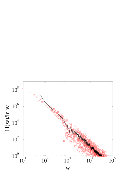
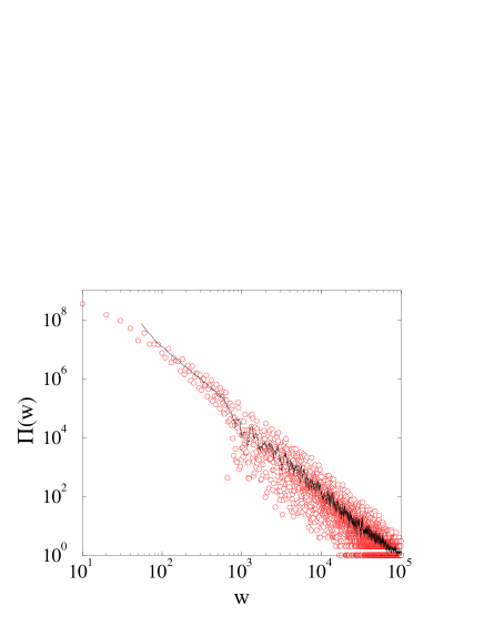
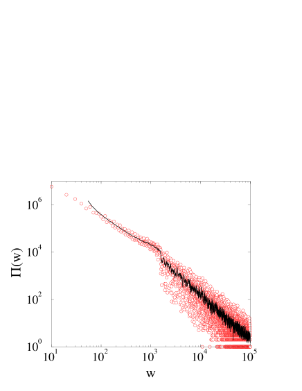
In Fig. 3, we show our data for the distribution of link weights for the representative cases of $\lambda=0$, $1$, and $-0.5$. The data shown are based on $10^{4}$ network realizations with $N=10^{6}$ for $\lambda=0$ and 1, while $N$ is limited to 25,000 for the $\lambda=-1/2$ due to the broadness of the link weight distribution. The data shows considerable small-scale variation because of the previously-mentioned fluctuations in the number of divisors of the integers; thus we also examined the locally averaged distribution given by Eq. (12). While this construction smooths the distribution, exponent estimates based on the smoothed distribution are nearly identical to those found for the raw distribution ($\Pi(w)$ in Eq. (11)) and thus we quote results based on the analysis of the latter.

For $\lambda=0$, a power-law fit to the data for $\Pi(w)/\ln w$ gives $\Pi(w)/\ln w\sim w^{-\chi}$, with $\chi\approx 2.3$, compared to the theoretical prediction from (22) of $\chi=2$. For $\lambda=1$, we find $\Pi(w)\sim w^{-\chi}$, with $\chi\approx 2.23$, while the theoretical prediction from (22) is $\chi=2.5$. Finally, for $\lambda=-0.5$, a simple power law fit to the raw distribution in Fig. 3 is clearly an oversimplification. However, a power-law fit to all the data gives $\chi=1.39$, close to the theoretical prediction of $\chi=1.5$. Overall, the agreement between the predictions of Eq. (22) and simulation results is surprisingly good, given the vagaries of these distributions.

Figure 4: The node strength $s(k)$ versus $k$ for a network of $N=10^{7}$ nodes with $\lambda=0$, and the contributions to this strength from incoming and outgoing links, as given by the two terms in Eq. (25) ($\square,\bullet,\Delta$ respectively). Inset: $s(k)_{\rm in}$ divided by $k^{2}\ln k$.

Figure 5: The node strength $s(k)$ and its contribution from incoming and outgoing links ($\square,\bullet,\Delta$ respectively) for the cases of $\lambda=1$ (upper) and $-2/3$ (lower), both with $N=10^{7}$.

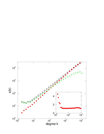
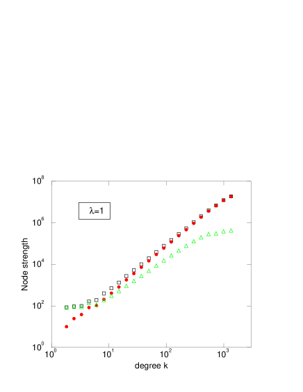
We also numerically calculate the node strength as function of the degree $k$. In Fig. 4 we show the results for $\lambda=0$ for a network of $N=10^{7}$ nodes. As a check of Eq. (27), the contribution to the node strength from the outgoing links was fit with form $s_{\rm out}(k)\sim k^{\beta}(\ln k_{\rm max}-\ln k)$. Using a non-linear curve fitting package, we obtain $\beta=1.9$ and $k_{\rm max}=13,000$. This value of $k_{\rm max}$ is very close to what we observed numerically (10,900) for the maximum degree over all 1000 realizations of the network. Overall, the data for $s_{\rm out}(k)$ agrees reasonably well with the theoretical prediction from Eq. (27) with $\beta=2$.

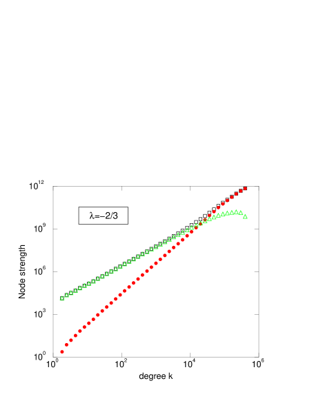
In Fig. 5 we show the node strength for two other representative values of $\lambda$. For the case of $\lambda=1$, both $s(k)$ and $s_{\rm out}(k)$ grow as $k^{2}$, as predicted by Eqs. (27) and (30). For the case of $\lambda=-2/3$, $s_{\rm out}(k)$ grows as $k^{4/3}$, as predicted by (27), while $s_{\rm in}(k)$ grows slightly faster than $k^{2}$, which is consistent with the $k^{2}\ln k$ growth given in Eq. (29). Notice also that the point where $s_{\rm in}(k)$ and $s_{\rm out}(k)$ intersect moves to larger $k$ as $\lambda$ decreases. This crossover point also coincides with $k_{\rm max}$ and the behavior of $k_{\rm max}$ on $\lambda$ is consistent with the prediction $k_{\rm max}\sim N^{1/(2+\lambda)}$.

Figure 6: The node strength for $\theta=0.5$. The left panel shows the case $\lambda=0$ and the right $\lambda=-2/3$, both for networks of size $N=10^{6}$. The node strength $s(k)$ and its contribution from incoming and outgoing links are denoted by $\square,\bullet$ and $\Delta$ respectively.

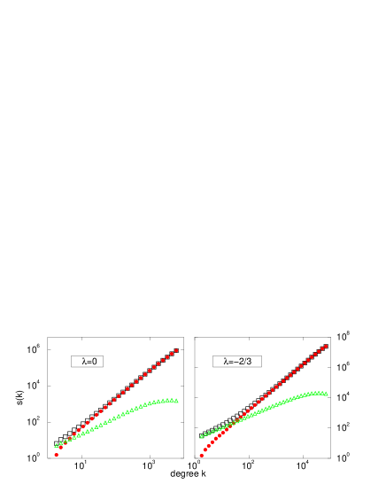
While most of our discussion has considered the case where the exponent $\theta=1$, there are examples of real networks, such as the E coli metabolic networks macdonald and the airline route network orsay , where the correlations between node degree and link weight seem to follow $w_{ij}=(k_{i}k_{j})^{1/2}$, that is $\theta=0.5$. To test the predictive power of our analytical approach also for the case of $\theta<1$, we investigate the scaling of node strength as a function of node degree for $\theta=1/2$ for the two specific examples of $\lambda=0$ and $\lambda=-2/3$ (Fig. 6). Our analytical results for the outgoing node strength are $s_{\rm out}(k)\sim k$ ($\lambda=0$) and $s_{\rm out}(k)\sim k^{5/6}$ ($\lambda=-2/3$), in good agreement with the best fits of $s_{\rm out}(k)\sim k^{0.9}$ and $s_{\rm out}(k)\sim k^{0.8}$, respectively.

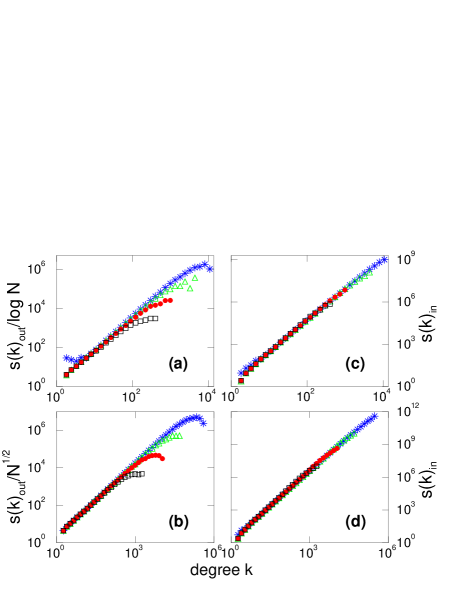
As a further test of our theoretical predictions, we show data for the node strength in which we attempt finite-size scaling (Fig. 7). In panel (a), the data for $\lambda=0$ is consistent with the asymptotic behavior of $s_{\rm out}(k)/\ln N\sim k^{2}$ given in Eq. (27). The departure from data collapse arises from the correction term in this equation. In panel (b), the data for $\lambda=2/3$ is now consistent with the form $s_{\rm out}(k)/N^{1/2}\sim k^{4/3}-k^{2}/N^{1/2}$ given in Eq. (32). The departure from data collapse is due to the influence of the correction term in $s_{\rm out}(k)$. Panel (c) shows the expected scaling behavior of $s_{\rm in}(k)\sim k^{2}\ln k$ given in Eq. (29). Curiously, this same behavior also occurs for the case of $\lambda=-2/3$.

VI Summary

We studied the statistics of growing networks in which each link $ij$ in the network has an associated weight $(k_{i}k_{j})^{\theta}$, where $k_{i}$ and $k_{j}$ are the node degrees at the endpoint of the link $ij$. We also characterized a node by its strength, defined as the sum of the weights of the links that are attached to this node. The link weights and node strengths provide new metrics with which to characterize heterogeneous networks. The motivation for considering these properties stems from a number of real-world examples, such as airline route networks or metabolic networks, in which the flow capacity of each link is different.

Figure 7: Finite size scaling of the node strength contribution from outgoing ((a) and (b)) and incoming ((c) and (d)) links for $\lambda=0$ (upper panels) and $\lambda=-2/3$ (lower panels). The network sizes are $N=10^{4},10^{5},10^{6}$ and $10^{7}$ ($\square,\bullet,\Delta,\ast$ respectively).

We focused on developing an analytical understanding of the link weights and node strengths as a function of the underlying growth mechanism of the network. Much of our analytical results are obtained by adapting previously-derived results for node degree correlations to the link weights and node strengths. Generically, we found that the total network weight grows faster than linearly with the total number of nodes $N$. Strictly linear growth of the total weight on $N$ occurs for networks whose degree distribution decays relatively quickly in $k$ for large $k$. The distribution of link weights has a power-law tail that is modified by a logarithmic correction for $\lambda=0$. There is also a strange and, as of yet, unexplained anomaly in this distribution when $\lambda<0$. There are also small-scale fluctuations in the link weight distributions that are caused by the granularity in the number of ways that a given link weight can be factored into a product of the degrees of the endpoint nodes.

A calculational approach in the same spirit as that used for the link weights was also applied to determine the node strength. For $\lambda\geq 0$, the node strength scales as $k^{2}$, with a logarithmic correction in the case of $\lambda=0$, while for $\lambda<0$, the node strength has a more complicated scaling behavior. The node strength can also be decomposed into contributions from the outgoing link and a contribution from incoming links. Only the former is amenable to a complete analytical treatment in terms of the two-node correlation function, while the latter requires knowledge of many-node correlations. We expect that these many-node correlation functions can be computed withing a rate equation approach.

VII Acknowledgments

PLK and SR are grateful to NSF grant DMR0227670 for partial support of this work.

Appendix A Lower Bound for The Total Link Weight

Our calculation for the total network weight relied on the distribution $n_{k,l}$ that was obtained in Ref. KR . We also made use of the cutoff $k_{\rm max}$ that applies for the degree distribution $n_{k}$ KR-finite . Thus the application of this cutoff to $n_{k,l}$ could in principle be questioned. Here we establish (for the simplest $\lambda=0$ model) a rigorous lower bound for the total weight of a network using only the well-known properties of the degree distribution.

Let $W(N)$ be the average total weight of the network with $N$ nodes. The next node will link to a target node of degree $k$ with probability $\frac{1}{2}\,kn_{k}$. The degree of the target node then increases $k+1$, so that the average weight of the new link is $\sum(k+1)\times(kn_{k})/2$. The increase of the degree of the target node ($k\to k+1$) implies that the weights of the $k$ current links that end at the target node will also increase; we denote this corresponding average increase by $(\ldots)$. Thus

$$W(N+1)=W(N)+\sum\frac{1}{2}\,k(k+1)n_{k}+(\ldots)$$ (33)

We shall ignore the positive increment $(\ldots)$ since its calculation requires knowledge of the distribution $n_{k,l}$. By this approximation we will derive the lower bound rather than the true asymptotic.

Equation (33), in conjunction with the well-known expression for the degree distribution

$$n_{k}=\frac{4}{k(k+1)(k+2)}\,,$$ (34)

then gives

$$W(N+1)>W(N)+\sum\frac{2}{k+2}.$$ (35)

For the degree distribution, the location of the cutoff $k_{\rm max}\sim N^{1/2}$ is well established. (Even the full scaling form $n_{k}(N)=n_{k}\,F(k/\sqrt{N})$ is known analytically KR-finite .)  Thus $W(N+1)-W(N)>\ln N$, so that the lower bound for the total weight is

$$W(N)>N\ln N.$$ (36)

This bound exhibits a slower growth than the prediction of Eq. (6) but it proves that the total weight of a network grows faster than linearly in $N$.

For the general case where the attachment rate as the form $A_{k}=k+\lambda$, the tail of the degree distribution is given by $n_{k}\sim k^{-3-\lambda}$. For $\lambda>0$ this asymptotic form for the degree distribution implies that the sum $\sum k(k+1)n_{k}$ converges, leading to the lower bound $W(N)>N$. This gives the same scaling behavior as the actual asymptotic behavior of Eq. (9). For $\lambda<0$, the sum $\sum k(k+1)n_{k}$ diverges and we use the cutoff $k_{\rm max}\sim N^{1/(2+\lambda)}$ to obtain $\sum k(k+1)n_{k}\sim N^{-\lambda/(2+\lambda)}$. This then gives the lower bound $W(N)>N^{2/(2+\lambda)}$, a result that also agrees with the actual asymptotic behavior in Eq. (9).

References

- (1) See e.g., R. Albert and A.-L. Barabási, Rev. Mod. Phys. 74, 47 (2002); S.N. Dorogovtsev and J. F. F. Mendes, Adv. Phys. 51, 1079 (2002). S. N. Dorogovtsev and J. F. F. Mendes, Evolution of networks: From biological nets to the Internet and WWW (Oxford University Press, Oxford, 2003); R. Pastor-Satorras and A. Vespignani, Evolution and structure of the Internet: A statistical physics approach (Cambridge University Press, Cambridge, 2004).
- (2) M. E. J. Newman, Phys. Rev. E 64, 016131 (2001); ibid, 64, 016132 (2001).
- (3) A.-L. Barabási, H. Jeong, Z. Neda, E. Ravasz, A. Schubert, and T. Vicsek, Physica A 311, 590 (2002).
- (4) See R. Guimera, M. Sales-Pardo, and L. A. N. Amaral, cond-mat/0312535 for a recent quantitative study of the airport network.
- (5) A. Barrat, M. Berthelemy, and A. Vespignani, Proc. Natl. Acad. Sci. 101, 3747 (2004); Phys. Rev. Lett. 92, 228701 (2004).
- (6) L. R. Ford and D. R. Fulkerson, Flows in Networks (Princeton University Press, Princeton, N.J., 1962)
- (7) R. K. Ahuja, T. L. Magnanti, and J. B. Orlin, Network Flows: Theory, Algorithms, and Applications (Prentice Hall, Englewood Cliffs, N.J., 1993).
- (8) P. J. Macdonald, E. Almaas, and A.-L. Barabási, cond-mat/0405688.
- (9) J. D. Noh and H. Rieger, Phys. Rev. E 66, 066127 (2002).
- (10) D. Zheng, S. Trimper, B. Zheng, and P. M. Hui, Phys. Rev. E 67, 040102(R) (2003).
- (11) M. E. J. Newman, cond-mat/0407503.
- (12) M. Baiesi and M. Paczuski, physics/0408018.
- (13) A. E. Motter, C. Zhou, and J. Kurths, cond-mat/0406207.
- (14) A. Barrat, M. Berthelemy, and A. Vespignani, cond-mat/0406238; cs.NI/0405070.
- (15) T. Antal and P. L. Krapivsky, cond-mat/0408285.
- (16) P. L. Krapivsky and S. Redner, Phys. Rev. E 63, 066123 (2001).
- (17) A.-L. Barabási and R. Albert, Science 286, 509 (1999).
- (18) H. A. Simon, Biometrica 42, 425 (1955); reprinted in H. A. Simon, Models of Man (Wiley, New York, 1957).
- (19) P. L. Krapivsky and S. Redner, Computer Networks 39, 261 (2002).
- (20) P. L. Krapivsky and S. Redner, J. Phys. A 35, 9517 (2002).
- (21) G. H. Hardy and E. M. Wright, An Introduction to the Theory of Numbers (Oxford University Press, Oxford, 1979).
- (22) M. R. Schroeder, Number Theory in Science and Communication (Springer-Verlag, Berlin, 1986).
- (23) M. E. J. Newman, Phys. Rev. Lett. 89, 208701 (2002); Phys. Rev. E 67, 026126 (2003).