Gradient Networks

Abstract

We define gradient networks as directed graphs formed by local gradients of a scalar field distributed on the nodes of a substrate network $G$. We derive an exact expression for the in-degree distribution of the gradient network when the substrate is a binomial (Erdős-Rényi) random graph, $G_{N,p}$. Using this expression we show that the in-degree distribution $R(l)$ of gradient graphs on $G_{N,p}$ obeys the power law $R(l)\propto l^{-1}$ for arbitrary, i.i.d. random scalar fields. We then relate gradient graphs to congestion tendency in network flows and show that while random graphs become maximally congested in the large network size limit, scale-free networks are not, forming fairly efficient substrates for transport. Combining this with other constraints, such as uniform edge cost, we obtain a plausible argument in form of a selection principle, for why a number of spontaneously evolved massive networks are scale-free. This paper also presents detailed derivations of the results reported in Ref. TB04 .

I Introduction

It has recently been recognized AB02 ; N03 ; DM03 that a large number of systems are organized into structures best described by complex networks, or massive graphs. Many of these networks, also called scale-free networks, such as citation networks R98 , the www AJB00 , the internet FFF99 , cellular metabolic networks JTAOB00 ; W01 , the sex-web LESAA03 , the world-wide airport network GMTA03 ; GA04 , and alliance networks in the U.S. biotechnology industry PWKO03 , possess power-law degree distribution, $P(k)\sim k^{-\gamma}$ BA99 . Scale-free networks are very different from pure random graphs, which are well studied in the mathematical literature B01 , and which have “bell curve” Poisson degree distributions. Therefore, it is natural to ask: Why do scale-free networks emerge in nature?

The diverse range of systems for which scale-free networks are important suggests that perhaps there is a simple common reason for their development. Generally, real-world networks do not form or evolve simply by purely random processes. Instead, networks develop in order to fulfill a main function. Often that function is to transport entities such as information, cars, power, water, forces, etc. It is thus plausible that the structure that the network develops (scale-free in particular) will be one that ensures efficient transport. Recent studies that explore the connection between network topology and flow efficiency were done by a number of researchers, including Valverde and Solé VS04 in the context of the internet, by Valverde Ferrer Cancho and Solé VFS02 in the context of software architecture graphs, and Guimerà et.al. GMTA03 in the context of the world-wide airport network. All these studies clearly show that the flow optimization dynamics which attempts to maintain the overall efficiency, will induce strong constraints on the structural evolution of the network.

In this paper, we investigate the processing efficiency of flows on networks when the flows are generated by gradients of a scalar field distributed on the nodes of a network. This approach is motivated by the idea that transport processes are often driven by local gradients of a scalar. Examples include electric current which is driven by a gradient of electric potential, and heat flow which is driven by a gradient of temperature. The existence of gradients has been also shown to play an important role in biological transport processes, such as cell migration N84 : chemotaxis, haptotaxis, and galvanotaxis (the later was shown to play a crucial role in morphogenesis).

Naturally, the same mechanism will generate flows in complex networks as well. Besides the obvious examples of traffic flows, power distribution on the grid, and waterways, we present two less known examples of systems where gradient-induced transport on complex networks plays an important role: 1) Diffusive load balancing schemes used in distributed computation RSW98 (and also employed in packet routing on the internet), and 2) Reinforcement learning on social networks with competitive dynamics ATBK03 . In the first example, a computer (or a router) asks its neighbors on the network for their current job load (or packet load), and then the router balances its load with the neighbor that has the minimum number of jobs to run (or packets to route). In this case the scalar at each node is the negative of the number of jobs at that node, and the flow occurs in the direction of the gradient of this scalar in the node’s network neighborhood. In the second example, a number of agents/players who are all part of a social network, compete in an iterated game based with limited information ATBK03 . At every step of the game each agent has to decide who’s advice to follow before taking an action (such as placing a bet), in its circle of acquaintances (network neighborhood). Typically, an agent will try to follow that neighbor which in the past proved to be the most reliable. That neighbor is recognized using a reinforcement learning mechanism: a score is kept for every agent measuring its past success at predicting the correct outcome of the game, and then each agent follows the advice of the agent in its network neighborhood which has the highest score ATBK03 accumulated up to that point in time. In this case, the scalar is the past success score kept for each agent.

The remainder of this paper is organized as follows. In Section II we systematically build a framework for analyzing the properties of gradient flows on networks, which, as it will be demonstrated, generically organizes itself into a directed network structure without loops. In Section III, we obtain the exact expression for the in-degree distribution of the gradient flow network on binomial random graphs and show that in a certain scaling limit the gradient flow network becomes a scale-free network. We also discuss possible connections of this result to sampling biases in trace-route measurements that have been used to infer the topology of the internet. Finally, in Section IV we study how the structure of a network affects the efficiency of its transport properties, and offer a possible explanation in the form of a selection principle for the emergence of real-world scale-free networks.

II Definition of a Gradient Network

Let us consider that transport takes place on a fixed network $G=G(V,E)$ which we will call in the remainder, the substrate graph. It has $N$ nodes, $V=\{0,1,...,N-1\}$ and the set of edges $E$ is specified by the adjacency matrix ${\bf A}=\{a_{ij}\}$ ($a_{ij}=1$ if $i$ and $j$ are connected, $a_{ij}=0$ otherwise, and $a_{ii}=0$). Given a node $i$, we will denote its set of neighbors in $G$ by $S_{i}^{(1)}=\{j\in V\;|\;a_{ij}=1\}$. Let us also consider a scalar field (which could just as well be called ‘potential landscape’) ${\bf h}=\{h_{0},..,h_{N-1}\}$ defined on the set of nodes $V$, so that every node $i$ has a scalar value $h_{i}$ associated to it.

We define the gradient $\nabla h_{i}$ of the field h in the node $i$ to be the directed edge $\nabla h_{i}=(i,\mu(i))$ which points from $i$ to that neighbor, $\mu(i)\in S_{i}^{(1)}\cup\{i\}$ on $G$ at which the scalar field has the maximum value in $S_{i}^{(1)}\cup\{i\}$, i.e.:

$$\mu(i)=\underset{j\in S^{(1)}_{i}\cup\{i\}}{\mbox{argmax}}(h_{j}),$$ (1)

see Fig. 1. According to its classical definition, a gradient vector points in the direction of the steepest ascent at a point on a continuous ($d$-dimensional) landscape. The above definition is a natural generalization to the case when the continuous landscape is replaced by a graph.

Note that $\mu(i)=i$, if $i$ has the largest scalar value in its neighborhood (i.e. in the set $S_{i}^{(1)}\cup\{i\}$), and in this case the gradient edge is a self-loop at that node. Since ${\bf h}$ always has a global maximum, there is always at least one self-loop. It is possible that Eq. (1) has more than one solution (several equal maxima) in the case of which we say that the scalar field is degenerate. In this paper we deal only with non-degenerate fields, which is typical when for example ${\bf h}$ is a continuous stochastic variable.

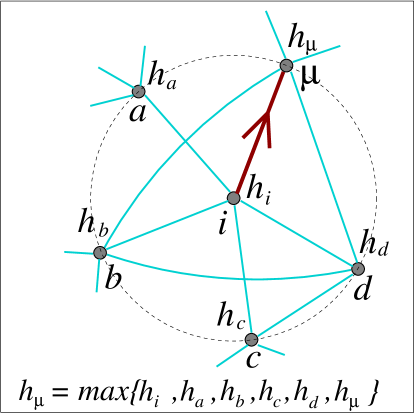
Figure 1: Definition of a gradient on a network. The gradient at node $i$ is a directed edge pointing towards the maximum value of the scalar (node $\mu$) in the node’s neighborhood.

This allows us to define: the set ${\bf F}$ of gradient edges on $G$, together with the vertex set $V$ form the Gradient Network, $\nabla G=\nabla G(V,{\bf F})$.

Assuming that all edges have the same ‘conductance’, or transport properties, the gradient network will be the substructure of the original network which at a given instant will channel the bulk of the flow, and thus alternatively can be called as the maximum flow subgraph.

In general, the scalar field will be evolving in time, due to the gradients generated currents, and also to possible external sources and sinks on the network (for example packets are generated and used up at nodes, but they can also be lost). As a result, the gradient network $\nabla G$ will be time-dependent, highly dynamic.

II.1 Some general properties of Gradient Networks

Here we will first show a number of fundamental structural properties valid for all instantaneous gradient networks, and then study the degree distribution of gradient networks generated by stochastic scalar fields on random graphs, and scale-free networks. This will lead us to show that scale-free networks are more efficient substrates for transport than random graphs. The first important observation we make about gradient networks is:
Non-degenerate gradient networks form forests (i.e., there are no loops in $\nabla G$, and it is a union of trees, more exactly of in-directed, planted pines).
To prove this statement, assume that on the contrary, there is a closed path $\gamma=\{\nabla h_{i_{1}},\nabla h_{i_{2}},...,\nabla h_{i_{m}}\}$, $m\geq 3$ made up only of directed edges from $\bf F$, see Fig. 2. Let $i_{k}$ be the node on this path for which $h_{i_{k}}=\min\{h_{i_{1}},h_{i_{2}},...,h_{i_{m}}\}$. Node $i_{k}$ has exactly two neighbors on $\gamma$, nodes $i_{k\pm 1}$, but only one gradient direction, $\nabla h_{i_{k}}$ pointing away from $i_{k}$. Since $h_{i_{k\pm 1}}>h_{i_{k}}$, none of the neighbors $i_{k\pm 1}$ will have their gradient edges pointing into $i_{k}$. Since there are two edges, $(i_{k},i_{k-1})$ and $(i_{k},i_{k+1})$, and only one gradient edge from $i_{k}$, one of the edges must not be a gradient edge, and thus the loop is not closed, in contradiction with the assumption that $\gamma$ is a loop with only gradient edges. Using a similar reasoning we can show that for non-degenerate scalar fields, there is no continuous path in $\nabla G$ connecting two local maxima of the scalar field ${\bf h}$. This means that on a given tree of $\nabla G$ there is only one local maximum of the scalar, and it is the only node with a self-loop on that tree. As a consequence, the number of trees in the forest equals the number of local maxima of the scalar field ${\bf h}$ on $G$. The fact that $\nabla G$ is made of trees (no loops), is rather advantageous for existing analytical techniques, especially if we take into consideration that $\nabla G$ is the most important substructure driving the flow in the network. Note that unless there is exactly one local maximum (and thus global as well) of ${\bf h}$ on $G$, $\nabla G$ is disconnected into a number of trees and thus $\nabla G$ is not a spanning tree.

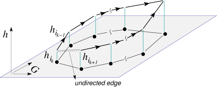
Figure 2: There cannot be loops in a non-degenerate $\nabla G$.

Since every node has exactly one gradient direction from it, the out-degree of every node on the gradient network is unity. It also means that $\nabla G$ has exactly $N$ nodes and $N$ edges (with at least one edge being a self-loop). However, the in-degree of a node $i$, which is the number of gradient edges pointing into $i$, can be anything in the range $k^{(in)}_{i}\in\{0,1,..,k_{i}\}$, where $k_{i}$ is the degree of node $i$ on $G$.

III The in-degree distribution of a gradient network on random graphs and random fields

In this section we show that when the substrate graph $G$ is a binomial random graph $G=G_{N,p}$ B01 , and ${\mathbf{h}}$ is an i.i.d. (meaning independent identically distributed) random field over $V$, given by a distribution $\eta(h)$, the in-degree distribution $R(l)=\mbox{Prob.}\{k^{(in)}_{i}=l\}$ of $\nabla G$ obeys the exact expression:

$$R(l)=\frac{1}{N}\sum_{n=0}^{N-1}\;{N-1-n\choose l}\left[1-p(1-p)^{n}\right]^{N-1-n-l}\left[p(1-p)^{n}\right]^{l}\;,$$ (2)

an expression independent on the particular form of the distribution for the scalars, $\eta(h)$. The binomial random graph (also coined in the physics literature as the Erdős-Rényi random graph) is constructed by taking all pairs $(i,j)$ of $N$ nodes and connecting them with probability $p$, independently from other links. Figure 3 shows the agreement between numerical simulations and the above exact expression.

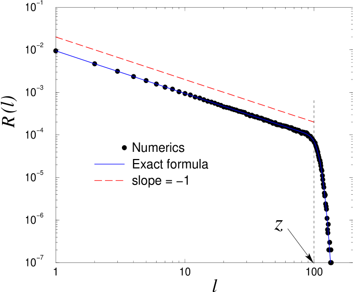
Figure 3: Comparison between the exact formula (2) and numerics. Here $N=1000$, $p=0.1$, ($z=100$). The numerical values are obtained after averaging over $10^{4}$ sample runs.

We will also show, that the gradient network $\nabla G$ becomes a scale-free (or power law) network with respect to the in-degree distribution, in the scaling limit $N\to\infty$ and $p\to 0$, such that $Np=z=const.\gg 1$. The in-degree distribution in this limit is described by the law:

$$R(l)\simeq\frac{1}{zl}\;,\;\;\;0<l\leq z\;.$$ (3)

a behavior which is also apparent from Fig. 3. This power-law is a rather surprising result, since the substrate graph is a random graph which is not scale-free, its degree distribution (in the same limit) being Poisson, with a well defined average degree $z$ (setting the scale) and faster than exponential decaying tails B01 .

A similar finding was reported in LBCX03 by Lakhina et.al. by repeating the trace-route measurements employed to sample the structure of the internet, on binomial random graphs. Lakhina et. al. find that the spanning trees obtained this way have a degree distribution that obeys the $1/k$ law. Later, in Ref. CM04 , Clauset and Moore have presented an analytical approach to derive the $1/k$ law. This suggests that perhaps there could be a mapping between the trace-route sampling generated graphs and gradient networks. Although it is not an exact mapping, a close connection can indeed be made, and this will form the subject of a forthcoming publication. The main warning sign coming from the trace-route observations is then the fact that trace-route sampling might not be the best way to measure the structure of the internet, given that on random binomial graphs it fails miserably to reproduce its degree distribution (instead of a Poisson, it gives a $1/k$ law). However, all is not lost, for the following reason: trace-route measurements of the internet suggested a power-law dependence for its degree distribution, $1/k^{\gamma}$ with an exponent of $\gamma$ taking values between 2 and 3, which is definitely not close to unity! This excludes the binomial random graph as a model for the internet. One might then wonder for what kind of graphs will trace-route measurements suggest a power-law dependence with an exponent $\gamma>2$? In Section III, we make the observation that if the substrate graph is a scale-free network with degree distribution given by $1/k^{\gamma}$ ($\gamma>2$) then the corresponding gradient network will also be a scale-free network with the same exponent $\gamma$. Using the above mentioned close mapping between trace-route trees and gradient networks (namely, trace-route trees can be interpreted as suitably constructed gradient networks) this suggests that at least the assumption that the internet is a power-law graph with exponent $\gamma>2$ is consistent with trace-route measurements. Certainly, the problem of sampling biases generated by trace-routes could be elucidated by answering the following question: are there non-power-law substrate graphs which would still generate scale-free trace-route trees with exponent $\gamma>2$? This is an open question wordy of further investigation.

IV Derivation of the exact expression

In this section we give a combinatorial derivation for formula (2). A more analytic and standard approach can be found in the Appendix, which was our original method, and it has inspired the combinatorial one presented below.

In order to calculate the in-degree distribution $R(l)$ this way, we first distribute the scalars on the node set $V$, then find those link configurations which contribute to $R(l)$ when building the random graph $G_{N,p}$ over these nodes.

Without restricting the generality we will calculate the distribution of in-links for node 0. Let us consider a set of $n$ nodes from $V$, that does not contain node 0, and it has the property that the scalar values at these nodes are all larger than $h_{0}$. We will denote this set by $\{\tau\}_{n}$. The complementary set of $\{\tau\}_{n}$ in $V\setminus\{0\}$ will be denoted by $C_{\{\tau\}_{n}}$, see Fig. 4.

In order to have exactly $l$ nodes pointing their gradient edges into node 0, we must fulfill the following conditions: first, they have to be connected to node 0 and, second, they must not be connected to the set $\{\tau\}_{n}$ (otherwise, they would be connected to a node with a scalar value larger than $h_{0}$, according to the definition of $\{\tau\}_{n}$). The probability for one node to fulfill these two conditions is $p(1-p)^{n}$, and since the links are drawn independently, for $l$ nodes this probability is $\left[p(1-p)^{n}\right]^{l}$. We must also require that no other nodes will have their gradient links pointing into node 0. Obviously, by definition, nodes from $\{\tau\}_{n}$ will not be pointing gradients into node 0. Therefore, we have to make sure, that none of the remaining $N-1-l-n$ nodes from $C_{\{\tau\}_{n}}$ will be pointing into 0. For one such node this will happen with probability $1-p(1-p)^{n}$. For all the $N-1-l-n$ such nodes this probability will be $\left[1-p(1-p)^{n}\right]^{N-1-l-n}$. Thus, given a specific set $\{\tau\}_{n}$, the probability of exactly $l$ in-links to node $0$ is:

$${N-1-n\choose l}\left[p(1-p)^{n}\right]^{l}\left[1-p(1-p)^{n}\right]^{N-1-l-n}\;.$$ (4)

The combinatorial factor in (4) counts the number of ways the set of $l$ nodes which point their gradient edges to node 0, can be chosen from $C_{\{\tau\}_{n}}$.

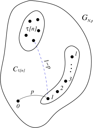
Figure 4: Schematic of the construction given in the main text.

The probability in (4) was computed by fixing $h_{0}$ and the set $\{\tau\}_{n}$. Next, we compute the probability $Q_{n}$ of such an event for a given $n$, while letting the field ${\bf h}$ vary according to its distribution. The probability for a node to have its scalar value larger than $h_{0}$ is:

$$\gamma(h_{0})=\int\limits_{h_{0}}dh\;\eta(h)$$ (5)

The probability to have exactly $n$ nodes with this property is given by:

$$\left[\gamma(h_{0})\right]^{n}\left[1-\gamma(h_{0})\right]^{N-1-n}\;.$$ (6)

The number of ways the $n$ nodes can be chosen from $V\setminus\{0\}$ is just the binomial ${N-1\choose n}$. Thus, the total probability $Q_{n}$ will be given by:

$$Q_{n}={N-1\choose n}\int dh_{0}\;\eta(h_{0})\;\left[\gamma(h_{0})\right]^{n}\left[1-\gamma(h_{0})\right]^{N-1-n}\;=\frac{1}{N}\;,$$ (7)

where the last equality in the above is obtained after performing the change of variables $du\equiv d\gamma(h_{0})=dh_{0}\;\eta(h_{0})$.

As a final step, by combining (7) with (4), and summing over all possible $n$ values, we arrive at (2).

IV.1 Derivation of the $1/l$ scaling for the in-degree distribution

In order to obtain the scaling $1/l$ valid in the limit $N\to\infty$, $p\to 0$, such that $z=pN=\mbox{const.}\gg 1$, for $0\leq l\leq z$, we will use the saddle point method. We write equation (2) first in the form $R(l)=\frac{1}{N}\sum_{n=1}^{N}r_{N}(n,l)$ and then exponentiate the argument. Using the Stirling’s formula to the first order ($\ln{(x!)}\approx x(\ln{x}-1)$), one obtains that $r_{N}(n,l)\approx e^{q_{N}(n,l)}$, where:

$$q_{N}(n,l) = (N-n)\ln{[(N-n)/e]}-l\ln{(l/e)}-(N-n-l)\ln{[(N-n-l)/e]}$$ (8)

$$+ (N-n-l)\ln{\left(1-p(1-p)^{n-1}\right)}+l[\ln{p}+(n-1)ln{(1-p)}]$$

To calculate the largest contributor under the sum in (2) we use the saddle point method: $\int dxe^{f(x)}\approx\sqrt{2\pi}e^{f(x_{0})}/\sqrt{-f^{\prime\prime}(x_{0})}$ where $f^{\prime}(x_{0})=0$. In our case we thus need to consider:

$$\left.\frac{\partial q_{N}(n,l)}{\partial n}\right|_{n^{*}(l)}=0$$ (9)

where $n^{*}(l)$ denotes the index of the maximal contributor for a given $l$. The difficulty we get into by trying to find $n^{*}(l)$ from (9) is that the equation cannot be solved explicitly for $n^{*}(l)$. To get around this, let us consider instead the derivative:

$$\left.\frac{\partial q_{N}(n,l)}{\partial l}\right|_{\hat{l}(n)}=0$$ (10)

defining $\hat{l}(n)$. Performing the derivation the solution is easily found as:

$$\hat{l}(n)=(N-n)p(1-p)^{n-1}\;.$$ (11)

Since $\hat{l}(n)$ is a monotonic function of $n$, it is invertible. ($\hat{l}^{\prime}(n)<0$). The inverse of (11), will be denoted by $\hat{n}(l)$. This means that:

$$\left.\frac{\partial q_{N}(n,l)}{\partial l}\right|_{\hat{n}(l)}=0\;.$$ (12)

Next, we observe that $\hat{l}(n)$ satisfies (9) when inserting it into its explicit expression. Accordingly, it will also be satisfied by $\hat{n}(l)$. Assuming that there is only one solution to (9) it thus follows that:

$$n^{*}(l)=\hat{n}(l)\;.$$ (13)

If we now calculate $q_{N}(n,l)$, at the saddle point, we find that $q_{N}(n^{*}(l),l)=0$ (using the fact that the parametric curve of the maximum can be written as either $(n^{*}(l),l)$ or $(n,\hat{l}(n))$ and thus calculating $q_{N}(n,\hat{l}(n))$). This means that we need to go one step further in the Stirling series, in order to calculate the leading piece of $e^{\ln{r_{N}(n,l)}}$ at the saddle point. For the saddle point itself, we use the same expression as previously (obtained with the first order Stirling approximation) because as it can be shown, the corrections introduced by the next term in the Stirling approximation are vanishing as $N\to\infty$ and therefore they will be neglected. Thus using the next order term in as well in the Stirling series ($\ln{(x!)}\approx x(\ln{x}-1)-\ln{(\sqrt{x})}+\ln{(\sqrt{2\pi})}$) and writing

$$\ln{r_{N}(n,l)}\approx q_{N}(n,l)+s_{N}(n,l)\;,$$ (14)

where $s_{N}(n,l)$ is the correction generated this way, we obtain:

$$e^{s_{N}(n^{*}(l),l)}=\frac{1}{\sqrt{2\pi}}\sqrt{\frac{N-n^{*}(l)}{N-n^{*}(l)-l}}\frac{1}{\sqrt{l}}=\frac{1}{\sqrt{2\pi}}\frac{1}{\sqrt{l}}+{\cal O}\left(\frac{\ln{z}}{z}\right)\;.$$ (15)

Calculating the second derivative $\partial^{2}q_{N}(n,l)/\partial n^{2}$ at the point (11), one finally obtains:

$$\frac{\partial^{2}q_{N}(n,l)}{\partial n^{2}}=-l\frac{z^{2}}{N^{2}}-l\mathcal{O}\left(\frac{z}{N^{2}}\right)-l\mathcal{O}\left(\frac{z^{3}}{N^{3}}\right)$$ (16)

Combining (16) with (14), (15) in the saddle point formula, one obtains that:

$$R(l)\approx\frac{1}{zl},$$ (17)

valid in the domain $1\leq l\leq l_{c}$. The cutoff value $l_{c}$ is determined by the validity range of the saddle-point method: since the function $n^{*}(l)$ is monotonically decreasing, at $l=l_{c}$ it will hit the lowest allowed value by the range of the integral (or sum), namely, at $n^{*}(l_{c})=1$. Since $\hat{l}$ is the inverse function of $n^{*}$, it follows that

$$l_{c}=\hat{l}(n^{*}(l_{c}))=\hat{l}(1)=p(N-1)=z$$ (18)

meaning that the cutoff for the $1/l$ scaling law happens at $z$, which is indeed confirmed by the numerical simulations shown in Fig. 3.

V Scale-free networks: results of a selection mechanism?

If the substrate graph is a scale-free network (here we used the Barabási-Albert (BA) process with parameter $m$ to generate the scale-free network AB02 , but others will lead to similar conclusions as long as $\gamma>2$), the gradient graph will still be a power-law. Here $m$ is the number of “stubs” of an incoming node which will attach preferentially to the existing network in the growth process. Figure 5 shows the in-degree distribution of the corresponding gradient networks (for $m=1$ and $m=3$, lines-markers) which are to be compared with the degree distribution of the substrate network itself (lines). One immediate conclusion is that the gradient network is the same type of structure as the substrate in this case, i.e., it is a scale-free (power law) graph with the same exponent!

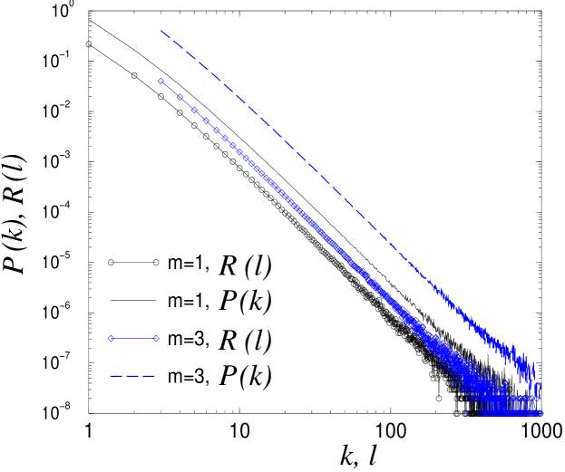
Figure 5: The degree distributions of the gradient network ($R(l)$) and the substrate ($P(k)$), when the substrate is a BA scale-free graph with parameter $m$ ($m=1,3$). Here $N=10^{5}$, and the average was performed over $10^{3}$ samples.

If $N_{l}^{(in)}$ denotes the number of nodes with $l$ in-links, the total number of nodes receiving gradient flow will be $N_{receive}=\sum_{l\geq 1}N_{l}^{(in)}$. The total number of gradient edges generated (total flow) is simply $N_{send}=N$ because every node has exactly one out-link.

If the flow received by a node has to be processed, it will happen at a finite rate. For example, a node receiving a packet, has to read off its destination and find out to which neighbor to send it. This is a physical process and takes a non-zero amount of time. Thus, if a node receives too many packets per unit time, they will form a queue, and long queues will generally cause delays in information transmission and thus leads to congestion, or jamming. An important question then arises: Can the topology of the underlying substrate graph influence the level of congestion in the network?
The answer is yes, as illustrated through the following trivial examples. a) If the network was a star-like structure as in Fig. 6a), then obviously all pairs of nodes would be at most two hops from each other, which is advantageous from the point of view of shortest distance between sources and destinations (and also routing would be very simple), however it would not work for large networks, because the central node would have to handle all the traffic from the other nodes and would have to process an extremely large queue. b) On the contrary, if the network would have a ring-like structure as in 6b), then in average there would be one server per one client, a rather advantageous setup from the point of view of having no congestion, however, there would be no short distances for transmission. More importantly, for both structures in Fig. 6, the network is rather vulnerable: in case of a) the failure of the central node, and in the case of b) the failure of any node, would cause a complete breakdown of transmission.

Figure 6: Illustrating the influence of structure on flows. In a) the central node will have maximal congestion, while in b) there is no congestion.

To characterize this interdependence between structure and flow in more generality, we introduce the ratio $N_{receive}/N_{send}$, which, naturally, will be related to the instantaneous global congestion in the network. As explained above, if this ratio is small, then there will be only a few nodes ($N_{receive}$) processing the flow of many ($N_{send}$) others and therefore, long queues are bound to occur, leading to congestion.

If we assume that flows are generated by gradients in the network, we can define:

$$J=1-\left\langle\left\langle\frac{N_{receive}}{N_{send}}\right\rangle_{h}\right\rangle_{nw}=R(0)$$ (19)

as the congestion (or jamming) factor. Certainly, $J=1$ means maximal congestion and $J=0$ corresponds to no congestion, and we always have $J\in[0,1]$. Note that $J$ is rather a congestion pressure characteristic generated by gradients, than an actual throughput characteristic.

For the random graph substrate $G_{N,p}\;$, $J^{R}(N,p)=\frac{1}{N}\sum_{n=1}^{N-1}\left[1-p(1-p)^{n}\right]^{N-1-n}$. We can show that in the limit $p=const.$ and $N\to\infty$, $J^{R}(N,p)=1-\frac{\ln N}{N\ln\left(\frac{1}{1-p}\right)}\left[1+{\cal O}\left(\frac{1}{N}\right)\right]\to 1$, i.e., the random graph becomes maximally congested. When $z=Np$ is kept constant while $N\to\infty$, a good approximation is $J^{R}(z)=\lim_{N\to\infty}J^{R}(N,z/N)=\int_{0}^{1}dx\;e^{-z(1-x)e^{-zx}}$. The $J^{R}(z)$ function has a minimum at $z^{*}=2.8763...$, when $J^{R}(z^{*})=0.6295..$ and $J^{R}(0)=1$. Since $e^{zxe^{-zx}}$ is always bounded: $e^{zxe^{-zx}}\in\left[1,e^{1/e}\right]$, for all $x\geq 0$ and $z\geq 0$, $J^{R}(z)\geq\int_{0}^{1}dx\;e^{-ze^{-zx}}=\frac{1}{z}\left[Ei(-z)-Ei\left(-ze^{-z}\right)\right]$. Expanding for $z>>1$, we obtain: $J^{R}(z)\geq 1-\frac{\ln z+\mbox{\bf\mbox{ \em\tiny C}}}{z}-...\to 1$, (C is the Euler constant) i.e., the random graph asymptotically becomes maximally congested, or jammed. The latter result (up to corrections in $1/z$) can immediately be obtained if one uses directly the asymptotic form (17) and the fact that $R(0)\approx 1-\int_{1}^{z}dlR(l)$.

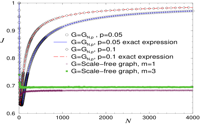
Figure 7: The congestion coefficient for random graphs ($\circ$, $p=0.05$; $\diamond$, $p=0.1$) and scale-free networks ($+$, $m=1$; $\square$, $m=3$).

For scale-free networks, however, the conclusion about jamming is drastically different. We find that the jamming (pressure) coefficient $J$ is always a constant, independent of $N$, in other words, scale-free networks are not prone to maximal jamming! In particular, $J^{SF}(N,m=1)=0.6839...$ and $J^{SF}(N,m=3)=0.6955...$ Figure 7 shows as comparison the congestion factors as function of network size both for random graph and scale-free network substrates.

Most real-world networks evolve more-or-less spontaneously (like the internet or www) and they also can reach massive proportions (order $10^{8}$ nodes). At such proportions, pure random graph structures would generate maximal congestion pressure (practically equal to unity) in the network and thus such substrates would be very inefficient for transport. Scale-free networks, however, have a congestion pressure which is a constant bounded well away from unity, and thus they are rather efficient substrates for transport. So why not all real-world networks are scale-free? Our analysis assumed that all edges have the same transport properties (conductance, or ”cost”), which is true for some networks like the www, the internet, and not true for others: power grid, social networks, etc. When there are weights on the edges (conductance or cost) the actual transport efficiency (determined by actual throughput) will strongly depend on those and therefore also select the network topology. Note that the congestion pressure depends on local properties of network topology (2-step neighborhoods). Thus we expect that all networks with similar 2-step neighborhood distributions would have similar gradient networks, not just the models studied here.

In summary, after introducing the concept of gradient flow networks, we have shown why certain complex networks might emerge to be scale-free. We do not give a specific mechanism for network evolution, which we believe to be network and process dependent, and therefore not universal. Instead, the network evolution mechanism is selected such, that the transport (the network’s main function) is efficient, while a number of constraints imposed by the specific nature of the network (edge cost, conductance, etc.) are obeyed.

In the case of the internet, if a router is constantly jammed, engineers will resolve the problem by connecting to the network other routers in its network vicinity, to share the load. This is a tendency to optimize the network flow locally. A series of such local optimization processes will necessarily have to constrain the global structure of the network. It seems that scale-free networks are within the class of networks obeying this type of constraint.

Acknowledgements

The authors acknowledge useful discussions with M. Anghel, B. Bollobás, P.L. Erdős, E.E. Lopez and D. Sherrington. Z.T. is supported by the US DOE under contract W-7405-ENG-36, K.E.B. is supported by the NSF through DMR-0406323, DMR-0427538, and the Alfred P. Sloan Foundation. B. K. and G. K. were supported in part by NSF through DMR-0113049, DMR-0426488, and the Research Corp. Grant No. RI0761. B.K. was also supported in part by the LANL summer student program in 2004 through US DOE Grant No. W-7405-ENG-36.

Appendix A An analytic derivation of the in-degree distribution

When calculating the degree distribution, we have to perform two averages: one corresponding to the scalar field disorder

$$\langle\bullet\rangle_{h}=\int dh_{0}...dh_{N-1}\;\eta(h_{0})..\eta(h_{N-1})\bullet\;,$$ (20)

and the other to an average over the network (graph ensemble):

$$\langle\bullet\rangle_{nw}=\sum_{a_{01}}...\!\!\sum_{a_{N-2N-1}}v(a_{01})...v(a_{N-2N-1})\bullet\;,$$ (21)

where $v(a)=p^{a}(1-p)^{1-a}$, $a\in\{0,1\}$ and $\sum_{a}\equiv\sum_{a=0}^{1}$. Here $G$ is the binomial random graph $G_{N,p}$ with $N$ nodes and link-probability $p$. The integrals in (20) are computed over the range of the scalar field and the summation in (21) is over all $N(N-1)/2$ pairs $(i,j)$ with $i<j\;$.

In order to calculate the in-degree distribution, we define first a counter operator for the in-links. Without restricting the generality we calculate the in-degree of the gradient network for node 0 namely, $k_{0}^{(in)}$. Let us introduce ${\bf B}={\bf I}+{\bf A}$, where ${\bf I}$ is the $N\times N$ identity matrix so $b_{ij}=\delta_{i,j}+a_{ij}$, and the quantities: $H_{i}(j)=1-b_{ij}+b_{ij}\;\theta(h_{0}-h_{j})$ for $i,j\in V$, and $i\in S^{(1)}_{0}$. Thus, the in-link counter can be written as:

$$k_{0}^{(in)}=\sum_{i=1}^{N-1}a_{0i}\prod_{j=1}^{N-1}H_{i}(j)\;.$$ (22)

With the aid of Fig. 8 we see that indeed this expression will count the number of gradient edges into node 0: $H_{i}(j)$ is zero only if the neighbor $j$ of $i$ (except node $0$) has a larger scalar value than node 0, i.e., $h_{0}<h_{j}$, otherwise $H_{i}(j)$ is equal to unity. Therefore a term under the sum in (22) will be non-zero if and only if for all neighbors $j$ of $i$ (i.e., $b_{ij}=1$) $h_{j}<h_{0}$ holds, making the edge $(i,0)$ to be the gradient edge for node $i$.

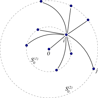
Figure 8: Node 0 has a gradient edge from $i$, if its scalar value is larger than the scalars of all its neighbors $j\neq 0$.

The probability that a node will have $l$ in-degree on the gradient network ${\bf F}$, is:

$$R(l)=\left\langle\left\langle\delta_{l,\;k^{(in)}_{0}}\right\rangle_{h}\right\rangle_{nw}=\int\limits_{-\pi}^{\pi}\frac{dq}{2\pi}e^{{\mathbf{i}}ql}\left\langle\left\langle e^{-{\mathbf{i}}qk^{(in)}_{0}}\right\rangle_{h}\right\rangle_{nw}\;.$$ (23)

First, we compute the average over the scalar field. (The order of the averages does not matter, however, it is formally easier this way.) Let us denote

$$L_{G}(q)=\left\langle e^{-{\mathbf{i}}qk^{(in)}_{0}}\right\rangle_{h}$$ (24)

We have:

$$L_{G}(q)=\int dh_{0}...\int dh_{N-1}\;\eta(h_{0})..\eta(h_{N-1})e^{-{\mathbf{i}}q\sum_{i=1}^{N-1}a_{0i}\prod_{j=1}^{N-1}\left[1-b_{ij}+b_{ij}\;\theta(h_{0}-h_{j})\right]}$$ (25)

Let $M_{i}(m)=\prod_{j=1}^{m}H_{i}(j)$. So

$$L_{G}(q)=\int dh_{0}...\int dh_{N-1}\;\eta(h_{0})..\eta(h_{N-1})e^{-{\mathbf{i}}q\sum_{i=1}^{N-1}a_{0i}M_{i}(N-1)}\;.$$ (26)

Using the recursion

$$M_{i}(m)=\left[1-b_{im}+b_{im}\;\theta(h_{0}-h_{m})\right]M_{i}(m-1)\;,$$ (27)

the integral over $h_{N-1}$ can be performed:

$$L_{G}(q)= \int\!\!dh_{0}...\int dh_{N-2}\;\eta(h_{0})..\eta(h_{N-2})$$ (28)

$$\times\left\{\gamma(h_{0})e^{-{\mathbf{i}}q\sum_{i=1}^{N-1}a_{0i}M_{i}(N-2)}+[1-\gamma(h_{0})]e^{-{\mathbf{i}}q\sum_{i=1}^{N-1}a_{0i}[1-b_{iN-1}]M_{i}(N-2)}\right\}$$

where $\gamma(x)=\int^{x}dy\;\eta(y)$. Performing all the integrals recursively, except for $h_{0}$, we obtain:

$$L_{G}(q)=\sum_{n=0}^{N-1}J(N,n)\!\!\!\!\sum_{[\tau]_{n}\in{\cal P}_{n}(N-1)}\!\!\!\!e^{-{\mathbf{i}}q\sum_{i=1}^{N-1}a_{0i}\prod_{j=1}^{n}(1-b_{i\tau(j)})}$$

where $J(N,n)=\int dh_{0}\eta(h_{0})[\gamma(h_{0})]^{N-1-n}[1-\gamma(h_{0})]^{n}$. Here $[\tau]_{n}=\{\tau(1),\tau(2),...,\tau(n)\}$ is a $n$-subset of the set $\{1,2,...,N-1\}$ and ${\cal P}_{n}(N-1)$ denotes the set of all $n$-subsets of $\{1,2,...,N-1\}$. We have $|{\cal P}_{n}(N-1)|={N-1\choose n}$. After a change of variables $u=\gamma(h_{0})$ and using $du=d\gamma(h_{0})=\eta(h_{0})h_{0}$ the integral $J(N,n)$ yields $J(N,n)=\frac{1}{N}{N-1\choose n}^{-1}$, i.e., the in-degree distribution is independent on the choice of the $\eta(h)$ distribution!

In the following, we perform the network average $\left\langle L_{G}(q)\right\rangle_{nw}$. For a fixed $n$-subset $[\tau]_{n}$, let us denote:

$$Z_{[\tau]_{n}}(q)\equiv\left\langle e^{-{\mathbf{i}}q\sum_{i=1}^{N-1}a_{0i}\prod_{j=1}^{n}(1-b_{i\tau(j)})}\right\rangle_{nw}\;.$$ (29)

Thus,

$$\left\langle L_{G}(q)\right\rangle_{nw}=\frac{1}{N}\sum_{n=0}^{N-1}{N-1\choose n}^{-1}\sum_{[\tau]_{n}\in{\cal P}_{n}(N-1)}Z_{[\tau]_{n}}(q)\;.$$ (30)

Let

$$T_{n}=[\tau]_{n}\cup\bigcup_{j=1}^{n}S^{(1)}_{\tau(j)}$$ (31)

be the set of vertices $[\tau]_{n}$ and its neighbors on $G$.

Note, that $\prod_{j=1}^{n}(1-b_{i\tau(j)})=1$ if and only if $i\not\in T_{n}$ otherwise it is zero. Therefore,

$$\sum_{i=1}^{N-1}a_{0i}\prod_{j=1}^{n}(1-b_{i\tau(j)})=\mbox{the nr. of neighbors of 0 {\em which do not belong to} }\;\;T_{n}.$$ (32)

From (21)

$$Z_{[\tau]_{n}}(q)=\sum_{a_{01}}...\!\!\sum_{a_{N-2N-1}}v(a_{01})...v(a_{N-2N-1})\;\prod_{i=1}^{N-1}e^{-{\mathbf{i}}qa_{0i}\prod_{j=1}^{n}(1-b_{i\tau(j)})}$$ (33)

Since $\tau(j)\neq 0$, ($[\tau]_{n}\in{\cal P}_{n}(N-1)$), the sums over the matrix variables $a_{0i}$ can be performed:

$$\sum_{a_{0i}}v(a_{0i})e^{-{\mathbf{i}}qa_{0i}\prod_{j=1}^{n}(1-b_{i\tau(j)})}=1-p+pe^{-{\mathbf{i}}q\prod_{j=1}^{n}(1-b_{i\tau(j)})}\;,$$ (34)

and therefore

$$Z_{[\tau]_{n}}(q)=\sum_{a_{12}}...\!\!\sum_{a_{N-2N-1}}v(a_{12})...v(a_{N-2N-1})\;\prod_{i=1}^{N-1}\left[1-p+pe^{-{\mathbf{i}}q\prod_{j=1}^{n}(1-b_{i\tau(j)})}\right]\;.$$ (35)

The set of vertices $\{1,2,...,N-1\}$ is split into two groups: $[\tau]_{n}$ and its complementary in $\{1,2,...,N-1\}$. Without changing anything, we can rename the vertices, such that $\{1,2,...,n\}=[\tau]_{n}$ and $C_{[\tau]_{n}}=\{n+1,n+2,...,N-1\}$ be the complementary set of $[\tau]_{n}$. It is easy to see that only cross-terms ($a_{ij}$ involving one node $i$ from $[\tau]_{n}$ and one node $j$ from $C_{[\tau]_{n}}$) give non-trivial contribution (i.e., different from unity) in (35). Thus:

$$Z_{[\tau]_{n}}(q)=\prod_{i=n+1}^{N-1}\sum_{a_{1i}}...\sum_{a_{ni}}v(a_{1i})...v(a_{ni})\left[1-p+pe^{-{\mathbf{i}}q\prod_{j=1}^{n}(1-a_{ji})}\right]$$ (36)

Let $\alpha_{1}=1-p$ and $\beta_{1}=p$. Then:

$$\sum_{a_{1i}}v(a_{1i})\left[\alpha_{1}+\beta_{1}e^{-{\mathbf{i}}q(1-a_{1i})...(1-a_{ni})}\right]=\alpha_{2}+\beta_{2}e^{-{\mathbf{i}}q(1-a_{2i})...(1-a_{ni})}$$ (37)

where $\alpha_{2}=(1-p)\alpha_{1}+p$ and $\beta_{2}=(1-p)\beta_{1}$. The summation over the rest of the matrix elements can be similarly performed to give (for a fixed node $i$)

$$\alpha_{n+1}+\beta_{n+1}e^{-{\mathbf{i}}q}\;.$$ (38)

The coefficients are determined from the recursion:

$$\left\{\begin{array}[]{ll}\alpha_{k}=(1-p)\alpha_{k-1}+p\;,&\;\;\alpha_{1}=1-p\\ \beta_{k}=(1-p)\beta_{k-1}\;,&\;\;\beta_{1}=p\end{array}\right.$$ (41)

which obeys $\alpha_{k}+\beta_{k}=1$ for all $k$. These recursions are easily solved:

$$\alpha_{n+1}=1-p(1-p)^{n}\;,\;\;\;\beta_{n+1}=p(1-p)^{n}\;.$$ (42)

Thus (38) becomes $1-p(1-p)^{n}+p(1-p)^{n}e^{-{\mathbf{i}}q}$. Since for all indices $i$ in (36) the result of the summations is the same, one finally obtains:

$$Z_{[\tau]_{n}}(q)=\left[1-p(1-p)^{n}\left(1-e^{-{\mathbf{i}}q}\right)\right]^{N-1-n}\;.$$ (43)

Because the result in (43) is not specific of the $[\tau]_{n}$ set, for all realizations of $[\tau]_{n}$, $Z_{[\tau]_{n}}(q)$ is the same expression, and thus the sum over all realizations of $[\tau]_{n}$ in (30) will generate the factor $|{\cal P}_{n}(N-1)|={N-1\choose n}$ which cancels the combinatorial factor in (30). Thus: $\left\langle L_{G}(q)\right\rangle_{nw}=\frac{1}{N}\sum_{n=0}^{N-1}Z_{[\tau]_{n}}(q)$. Plugging this into (23), and performing the integral over the $q$ variable we obtain:

$$R(l)=\frac{1}{N}\sum_{n=0}^{N-1}\;{N-1-n\choose l}\left[1-p(1-p)^{n}\right]^{N-1-n-l}\left[p(1-p)^{n}\right]^{l}$$ (44)

with the usual convention ${M\choose m}=0$ for $M<m$. Equation (44) is the exact expression for the in-degree distribution of the gradient network $\nabla G$.

References

- (1) Z. Toroczkai, K.E. Bassler, Nature, 428, 716 (2004).
- (2) R. Albert, A.L. Barabási, Rev. Mod. Phys. 74, 47 (2002).
- (3) M.E.J. Newman, SIAM Rev. 45, 167 (2003).
- (4) S.N. Dorogovtsev and J.F.F. Mendes, Evolution of Networks: From Biological Nets to the Internet and WWW, Oxford Univ. Press, Oxford, 2003.
- (5) S. Redner, Eur.Phys.J. B, 4, 131 (1998).
- (6) R. Albert, H. Jeong, and A.L. Barabási, Nature 401, 130 (1999); F. Menczer, Proc.Natl.Acad.Sci.USA, 99 14014 (2002); ibid. 101 5261 (2004).
- (7) M. Faloutsos, P. Faloutsos and C. Faloutsos Comp.Comm.Rev. 29, 251 (1999).
- (8) H. Jeong, B. Tombor, R. Albert, Z.N. Oltvai, A.-L. Barabási, Nature 407, 651 (2000)
- (9) A. Wagner, D.A. Fell, Proc. R. Soc. Lond. B, 268, 1803 (2001).
- (10) F. Liljeros, C.R. Edling, H.E. Stanley, Y. Aberg and L.A.N. Amaral, Nature 423, 606 (2003).
- (11) R. Guimerà, S. Mossa, A. Turtschi and L.A.N. Amaral, http://arxiv.org/abs/cond-mat/0312535.
- (12) R. Guimerà, and L.A.N. Amaral, Eur.Phys.J. B, 38, 381 (2004).
- (13) W. W. Powell, D. R. White, K. W. Koput and J. Owen-Smith Am.J.Soc. in press (2004).
- (14) A.L. Barabási and R. Albert, Science 286, 509 (1999).
- (15) B. Bollobás, Random Graphs, Second Edition, Cambridge University Press (2001).
- (16) S. Valverde and R.V. Solé, Eur.Phys.J.B, 38, 245 (2004).
- (17) S. Valverde, R. Ferrer Cancho and R.V. Solé, Europhys.Lett. 60, 512 (2002).
- (18) R. Nuccitelli, in Pattern Formation: A Primer in Developmental Biology, Ed. G.M. Malacinski, pp. 23, MacMillan, New York (1984).
- (19) Y. Rabani, A. Sinclair and R. Wanka, Proc.39th Symp. on Foundations of Computer Science (FOCS) pp. 694 (1998)
- (20) M. Anghel, Z. Toroczkai, K.E. Bassler and G. Korniss, Phys.Rev.Lett. 92, 058701 (2004).
- (21) A. Lakhina, J.W. Byers, M. Crovella, and P. Xie, Proc. IEEE Infocom (2003).
- (22) A. Clauset and C. Moore, http://arxiv.org/abs/cond-mat/0312674