Quantum Particles Constrained on Cylindrical Surfaces with Non-constant Diameter

Abstract

We present a theoretical formulation of the one-electron problem constrained on the surface of a cylindrical tubule with varying diameter. Because of the cylindrical symmetry, we may reduce the problem to a one-dimensional equation for each angular momentum quantum number $m$ along the cylindrical axis. The geometrical properties of the surface determine the electronic structures through the geometry dependent term in the equation. Magnetic fields parallel to the axis can readily be incorporated. Our formulation is applied to simple examples such as the catenoid and the sinusoidal tubules. The existence of bound states as well as the band structures, which are induced geometrically, for these surfaces are shown. To show that the electronic structures can be altered significantly by applying a magnetic field, Aharonov-Bohm effects in these examples are demonstrated.

I Introduction

Developments in the synthesis of nano-structured materials is ever expanding the list of structures which may be used for applications. Among other things, structures obtained as self-assembled interfaces in lyotropic liquid crystals, which are used as the templates of meso-porous materials, as well as structures made of bent graphites, including carbon nano-fullerenes, are intriguing examples. These structures are characterized by curved surfaces in nanometer scales and often possess a variety of geometrical properties. It is interesting to study the electronic properties related to the geometrical properties if the electron is constrained on the curved surfaces, because such unique settings may provide a new phenomena in quantum domain which can be pursued for electronic applications. We here consider the problem of quantum particle motion constrained on curved surfaces with the tubular topology and cylindrical symmetry.

We start with a model approach developed in Refs.jensen ; costa ; ikegami , in which the electron is assumed to be confined strongly to within a thin layer built over the surface. A limiting procedure that brings the thickness of the layer to be zero leads to the Hamiltonian in the form of the sum of a Laplace-Beltrami operator and an effective attractive potential energy associated with the local curvatures. These terms are written using double curvilinear coordinates on the surface. The stationary solutions of the Schr$\ddot{\rm o}$dinger equation are inevitably affected by the metric properties, curvatures, and topology of the surface. Previous studies reported that the effective potential energy can induce bound states whose localization centers are strongly curved parts of the surface. costa ; ikegami The discrete energy levels for bound states usually lie below the lowest edge of the essential (continuous) spectrum. The electronic structures can also be affected substantially by the global topology of the surface, because it restricts the ways in which the electronic wave propagates and interferes. This point, however, has not been studied comprehensively.

The purpose of this paper is to develop a basic formulation for curved surfaces with the tubular topology and cylindrical symmetry, and also to present some of its outcomes for simple examples. Our attention is focused on the case of tubular surfaces with non-constant diameter, namely, ones with non-vanishing Gaussian curvatures. The geometrical character of the surfaces dealt with in this paper is among the simplest and can be treated with relatively simple mathematics, though the results are not trivial. Within our formulation, it can be readily shown that there can be bound states lying inside the essential spectrum with a different angular momentum. The analyses of the electronic structures of curved surfaces with more complicated geometries, especially ones so called triply periodic minimal surfaces,aoki should resort to more elaborated group theoretical techniques. Our formulation is expected to provide some insight into further studies.

This paper is organized as follows. In Section 2, the basic Schr$\ddot{\rm o}$dinger equation for an electron strongly constrained on a curved surface is summarized briefly.jensen ; costa ; ikegami The equation is applied to a class of tubular surfaces with cylindrical symmetry in Section 3. By symmetry, the basic two-dimensional equation can be reduced to a one-dimensional form, where an axial magnetic field can also be taken into account. In Section 4 we study several specific examples and provide the functional form of the potential energy for each case. These specific problems are solved numerically, where we observe the existence of bound states at the strongly curved region on a surface. For periodically modulated structures, the relevant one-dimensional band structures as well as charge density distributions along the tubule are calculated. The electronic structures can be manipulated by tuning the applied magnetic field. The Aharonov-Bohm oscillations of the energy levels of the bound states are demonstrated. Further discussions are given in Section 5, and the conclusions in Section 6.

II One-particle motion constrained on a curved surface

Consider a two-dimensional manifold $\mathcal{M}$ embedded in the three-dimensional Euclidean space $E^{3}$ and assume a curvilinear surface coordinate system $q^{i}$ ($i=1,2$) on $\mathcal{M}$. Then the metric tensor $g_{ij}$ ($i,j=1,2$) is defined by ${\rm d}s^{2}=g_{ij}{\rm d}q^{i}{\rm d}q^{j}$ where ${\rm d}s$ is an infinitesimal distance. We write the principal curvatures as $\kappa_{i}$ ($i=1,2$). The quantum mechanics of a single electron which is constrained physically on $\mathcal{M}$ through a strong confining potential energy is described by the following Schr$\ddot{\rm o}$dinger equation, jensen ; costa ; ikegami

$$-\frac{\hbar^{2}}{2M}\frac{1}{\sqrt{g}}\frac{\partial}{\partial q^{i}}\sqrt{g}g^{ij}\frac{\partial}{\partial q^{j}}\psi(q^{1},q^{2})$$

$$-\frac{\hbar^{2}}{8M}(\kappa_{1}-\kappa_{2})^{2}\psi(q^{1},q^{2}) = E\psi(q^{1},q^{2}),$$ (1)

where $g=\det{(g_{ij})}$ and $(g^{ij})=(g_{ij})^{-1}$. The first term involves the Laplace-Beltrami operator which describes the propagation of waves through a curved surface with non-Euclidean metric. The second term is the attractive potential energy associated with the local curvature,vsclassical which essentially arises from the ’spread’ of the wave function perpendicular to the surface and thus is related to the uncertainty principle. The normalization condition for $\psi(q^{1},q^{2})$ is given by the integral

$$\int\int|\psi(q^{1},q^{2})|^{2}g^{\frac{1}{2}}{\rm d}q^{1}{\rm d}q^{2},$$ (2)

which should be unity for square integrable cases. Static magnetic fields can also be taken into account, in which case the equation becomes

$$\frac{1}{2M}\frac{1}{\sqrt{g}}\left(-i\hbar\frac{\partial}{\partial q^{i}}+\frac{e}{c}A_{i}\right)\sqrt{g}g^{ij}\left(-i\hbar\frac{\partial}{\partial q^{j}}+\frac{e}{c}A_{j}\right)$$

$$\times\psi(q^{1},q^{2})-\frac{\hbar^{2}}{8M}(\kappa_{1}-\kappa_{2})^{2}\psi(q^{1},q^{2})=E\psi(q^{1},q^{2}),$$ (3)

where $A_{i}$ are the components of the magnetic vector potential associated with the coordinates $q^{i}$.

III Surfaces with Cylindrical Symmetry

Now let us consider a class of smoothly curved surfaces with cylindrical symmetry, so that they are invariant under an arbitrary rotation around the $z$ axis. It is convenient to use the cylindrical coordinates $(r,\phi,z)$, with which the generator for a rotation around the $z$-axis is given by $l_{z}=-i\partial/\partial\phi$, the $z$-component of the angular momentum. Any of such surfaces can be specified by the set of coordinates $(z(x),r(x))$ as functions of the longitudinal surface coordinate $x$ taken perpendicular to the azimuthal coordinate, $\phi$. A given value of $x$ thus specifies a circle of radius $r(x)$ lying on $z=z(x)$ plane. If the function $z(x)$ has a monotonic dependence so that it is invertible, then the radius can be expressed as a function of $z$, $r=r(x(z))=r(z)$. This means that, in describing such a surface, we may use the $z$ coordinate as the longitudinal surface coordinate. We shall treat this particular case in more detail in the following.

For the cylindrical surface specified as $r=r(z)$, the surface metric ${\rm d}s^{2}=g_{zz}{\rm d}z^{2}+g_{\phi\phi}{\rm d}\phi^{2}$ is given by

$$g_{zz} = 1+{r^{\prime}(z)}^{2},$$

$$g_{\phi\phi} = r(z)^{2},$$ (4)

$$g\quad = r(z)^{2}(1+{r^{\prime}(z)}^{2}).$$

The principal curvatures of the surface are given by

$$\kappa_{1}=\frac{1}{r(z)\sqrt{1+{r^{\prime}(z)}^{2}}},\quad\kappa_{2}=-\frac{r^{\prime\prime}(z)}{(1+{r^{\prime}(z)}^{2})^{\frac{3}{2}}},$$ (5)

where $\kappa_{2}$ corresponds to the curvature along the longitudinal direction.

We shall consider a magnetic field which is applied to the system parallel to the $z$-axis, and suppose its magnitude is given by $B(r)$, a function of the radial coordinate $r$. In the symmetric gauge, the vector potential is given by

$$(A_{x},A_{y},A_{z})=\frac{\Phi(r)}{2\pi}\frac{1}{r^{2}}(-y,x,0),$$ (6)

where $\Phi(r)=\int^{r}_{0}2\pi r^{\prime}B(r^{\prime}){\rm d}r^{\prime}$ is the total flux passing through a disc of radius $r$. In the cylindrical coordinates $(r,\phi,z)$, the relevant components of the vector potential are given by

$$(A_{r},A_{\phi},A_{z})=(0,\frac{\Phi(r)}{2\pi},0).$$ (7)

This can be applied for an Aharonov-Bohm type magnetic field, $A_{\phi}=\Phi/2\pi$, as well as a uniform magnetic field, $A_{\phi}=Br^{2}/2$. The Schr$\ddot{\rm o}$dinger equation can now be written as

$$-\frac{\hbar^{2}}{2M}\left[\frac{1}{r\sqrt{1+{r^{\prime}}^{2}}}\frac{\partial}{\partial z}\frac{r}{\sqrt{1+{r^{\prime}}^{2}}}\frac{\partial}{\partial z}-\frac{1}{r^{2}}\left(l_{z}+\frac{e}{c\hbar}A_{\phi}\right)^{2}\right]$$

$$\times\psi(z,\phi)-\frac{\hbar^{2}}{8M}(\kappa_{1}-\kappa_{2})^{2}\psi(z,\phi)=E\psi(z,\phi),$$ (8)

where $l_{z}=-i\frac{\partial}{\partial\phi}$. Since $l_{z}$ commutes with the Hamiltonian (the rotational symmetry), we can assume as the form of the solution $\psi(z,\phi)=e^{im\phi}\psi_{m}(\phi)$, in which $m$ is the eigenvalue of $l_{z}$ and can take only integer values in order for the wave function to be single valued. Then the Schr$\ddot{\rm o}$dinger equation is written as

$$-\frac{\hbar^{2}}{2M}\left[\frac{1}{r\sqrt{1+{r^{\prime}}^{2}}}\frac{\rm d}{\rm dz}\frac{r}{\sqrt{1+{r^{\prime}}^{2}}}\frac{\rm d}{\rm dz}-\frac{\lambda_{m}(z)^{2}}{r^{2}}\right]\psi_{m}(z)$$

$$-\frac{\hbar^{2}}{8M}(\kappa_{1}-\kappa_{2})^{2}\psi_{m}(z)=E\psi_{m}(z),$$ (9)

where

$$\lambda_{m}(z)\equiv m+\frac{e}{c\hbar}A_{\phi}(r(z)).$$ (10)

This has a Sturm-Liouville form,

$$-\frac{\rm d}{{\rm d}z}\left[p(z)\frac{{\rm d}\psi_{m}(z)}{{\rm d}z}\right]+q(z)\psi_{m}(z)=\epsilon w(z)\psi_{m}(z),$$ (11)

where

$$\epsilon=\frac{2ME}{\hbar^{2}},$$ (12)

and

$$p(z) = \frac{r}{\sqrt{1+{r^{\prime}}^{2}}},$$

$$q(z) = \left[\frac{\lambda_{m}^{2}}{r^{2}}-\frac{1}{4}(\kappa_{1}-\kappa_{2})^{2}\right]w(z),$$ (13)

$$w(z) = r\sqrt{1+{r^{\prime}}^{2}}.$$

Hence by introducing the new variable $x$ as

$$x=\int^{z}\sqrt{\frac{w(z^{\prime})}{p(z^{\prime})}}{\rm d}z^{\prime}=\int^{z}\sqrt{1+{r^{\prime}(z^{\prime})}^{2}}{\rm d}z^{\prime},$$ (14)

Eq.(9) can be reduced to a simpler form,CourantHilbert

$$-\frac{{\rm d}^{2}}{{\rm d}x^{2}}y_{m}(x)+W_{m}(x)y_{m}(x)=\epsilon y_{m}(x),$$ (15)

where

$$y_{m}(x)=(p(z)w(z))^{\frac{1}{4}}\psi_{m}(z)=\sqrt{r(z)}\psi_{m}(z),$$ (16)

and

$$W_{m}(x) = \frac{q(z)}{w(z)}+\frac{1}{(p(z)w(z))^{\frac{1}{4}}}\frac{{\rm d}^{2}}{{\rm d}x^{2}}(p(z)w(z))^{\frac{1}{4}}$$ (17)

$$= \left(\lambda_{m}(z)^{2}-\frac{1}{4}\right)\frac{1}{r(z)^{2}}-\frac{1}{4}\kappa_{2}^{2}.$$ (18)

Eq.(15) has the form of a one-dimensional Schr$\ddot{\rm o}$dinger equation with a potential energy $W_{m}(x)$, where $x$ corresponds to the Euclidean line length along a curve on the surface with fixed $\phi$. Note that the second term in Eq.(17) turns out to be $(\kappa_{1}^{2}-2\kappa_{1}\kappa_{2}-1/r^{2})/4$, so that all terms including $\kappa_{1}$ are formally cancelled out in the last expression (18). The normalization condition for the wave function $y_{m}(x)$ is

$$2\pi\int|y_{m}(x)|^{2}{\rm d}x=1,$$ (19)

for square integrable cases.

IV Specific examples

We shall study several particular examples of curved surfaces with cylindrical symmetry by using the formulation presented above. The first and the simplest example is the catenoid, which gives one of the simplest examples of curved surfaces with zero mean curvature or minimal surfaces. The second example is the tubular surfaces whose diameter changes periodically along the cylindrical axis, in which the diameter function $r(z)$ is given by a sinusoidal form.

For each of these simple surfaces, the Schr$\ddot{\rm o}$dinger equation is solved numerically, using a finite difference method with appropriate boundary conditions. For instance, a Dirichlet or Neumann boundary condition (see Appendix A) can be used for the case of the catenoid, while the constant phase increment for Bloch states is used for the case of the sinusoidal surface.

IV.1 Catenoid

The catenoid is defined in its generalized form by the radius function $r(z)=a\cosh{z}$, in which $a$ ($>0$) specifies the aspect ratio. The surface is minimal if and only if $a=1$ (see Fig.1), corresponding to the original definition of the catenoid. Such surfaces can be thought of as simple geometrical models of pore structures common in physical systems. Note that the unit of length is taken as the characteristic depth of the pore.pore

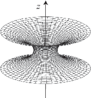
Figure 1: The catenoid surface defined by $r(z)=a\cosh{z}$ with $a=1$. The value of $a$ corresponds to the inner radius of the pore in unit of the characteristic pore depth along $z$.

The variable $x$ defined in Eq.(14) is given by

$$x=\int_{0}^{z}\sqrt{1+a^{2}\sinh^{2}z^{\prime}}{\rm d}z^{\prime}=-iE(iz,a^{2}),$$ (20)

where the function $E(\phi,k^{2})=\int^{\phi}_{0}\sqrt{1-k^{2}\sin^{2}\phi}{\rm d}\phi$ is the elliptic integral of the second kind. The potential energy function reads

$$W_{m}(x)=\left(\lambda_{m}^{2}-\frac{1}{4}\right)\frac{1}{a^{2}\cosh^{2}z}-\frac{1}{4}\frac{a^{2}\cosh^{2}z}{(1+a^{2}\sinh^{2}z)^{3}}$$ (21)

where $z$ implies a function of $x$. Note that in this expression the ’radial’ part and the ’longitudinal’ part compete with each other as $a$ is varied. The radial part, which is dominant when $a$ is small, decays outside the pore region of unit depth. Without magnetic field, this contribution is negative (attractive) for $m=0$ while it is positive (repulsive) for $m\neq 0$. This is plausible because in a narrow part of the catenoid the contribution of kinetic energy due to alternation of signs of a wave function around the axis becomes costly unless the wave function is effectively repelled from that region. This part also inherits some attractive contribution associated with the curvatures. On the other hand, the longitudinal part is dominant when $a$ is large, and it decays rapidly when $x$ exceeds $1/a$. This is purely the effect of the curvature in the longitudinal direction and independent of $m$ as well as the magnetic field.

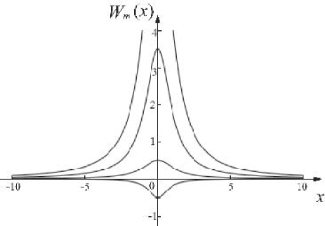
Figure 2: Effective potential energy curves $W_{m}(x)$ for catenoid when there is no magnetic field. These four curves corresponds to $m=0$ (bottom), $m=\pm 1$, $m=\pm 2$, and $m=\pm 3$ (top), respectively.

In the case of $a=1$, the above expressions reduce to

$$x=\int_{0}^{z}\cosh z{\rm d}z=\sinh z$$ (22)

and

$$W_{m}(x)=\left(\lambda_{m}^{2}-\frac{1}{4}\right)\frac{1}{1+x^{2}}-\frac{1}{4}\frac{1}{(1+x^{2})^{2}}.$$ (23)

This is the simplest form among the examples we have considered apart from a trivial straight tubule.exact? Several potential energy curves $W_{m}(x)$ for $a=1$ without magnetic field are shown in Fig.2. The minimal value of the potential energy for $m=0$, $W_{0}(0)=-1/4(1/a^{2}+a^{2})$, is maximal for $a=1$, so that the two contributions can be said to be balanced for this case.

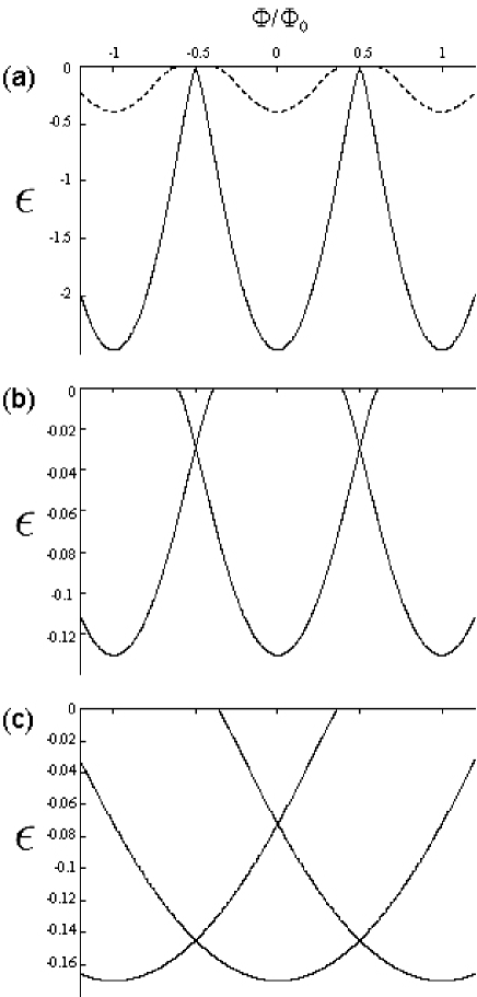
Figure 3: The dependence of the eigenenergies of the bound states on the Aharonov-Bohm flux through the pore of the catenoid, for (a) $a=0.25$, (b) $a=1.0$, and (c) $a=2.5$. Three congruent curves (shifted horizontally) correspond to $m=-1$, $0$, and $1$. For $a=0.25$, there exists the second bound state for each $m$ and is shown by a broken line.

We have numerically obtained the energy spectrum for the catenoid surfaces with several different values of $a$, where in most cases we have found one or several bound states centered around the constricted part of the surfaces.boundstate The energies of the bound states lie below the continuum $E>0$. For instance, one bound state is found for $a=1.0$ without magnetic field and the energy eigenvalue has been numerically estimated to $\epsilon\approx-0.13$.

For an Aharonov-Bohm type magnetic field, the magnetic field is non-zero only along the rotational axis, so that the surface is totally field-free. Hence, any solution of Eq.(II) can be given by a solution of the field free equation, (II) multiplied by the phase factor

$$\exp{\left(-\frac{ie}{\hbar c}\int^{q}_{q_{0}}\vec{A}\cdot{\rm d}\vec{l}\right)},$$ (24)

which will affect the boundary condition. In the case of cylindrical surfaces, this factor is given by

$$\exp{\left(-i\frac{e\Phi}{hc}\phi\right)},$$ (25)

which is independent of $z$. Note that the function $\lambda_{m}(z)$ in Eq.(9) is a constant

$$\lambda_{m}(z)\equiv\lambda_{m}=m+\frac{e\Phi}{hc},$$ (26)

and the energy spectrum is the superposition of the sub-spectra for all the allowed values of $\lambda$’s. This indicates that the energy spectrum oscillates as a function of flux $\Phi$ (Fig.3) and the period of oscillation is given by:

$$\Phi_{0}=\frac{hc}{e}\approx 2.07\times 10^{-11}{\rm Gauss}\cdot m^{2}.$$ (27)

In Fig.3 we show the energy eigenvalues of bound states as functions of the magnetic flux for $a=0.25$, $1.0$, and $2.5$. The energy eigenvalue is minimal when the total flux is zero and it increases rapidly with the magnetic flux. We can also see that the energy spectrum is less sensitive for larger $a$ consistent with the fact that the longitudinal part of $W_{m}(x)$ is field independent. In the case of uniform magnetic field the oscillation is suppressed for the magnetic flux passing through the tubule is no longer a constant along the axis direction if the radius is not constant.

IV.2 Sinusoidal tubules

We next consider the case of infinitely many pores along the tubule. This is achieved by taking a radius function of the sinusoidal form $r(z)=a+b\cos(z)$ with $a>b$ ($>0$), so that the diameter changes periodically along the axis. (See Fig.4.) The relevant variable $x$ is given by

$$x=\int^{z}_{0}\sqrt{1+b^{2}\sin^{2}z^{\prime}}{\rm d}z^{\prime}=E(z,-b^{2}).$$ (28)

Then the effective potential energy curve,

$$W_{m}(x)=\left(\lambda_{m}^{2}-\frac{1}{4}\right)\frac{1}{(a+b\cos z)^{2}}-\frac{1}{4}\frac{b^{2}\cos^{2}z}{(1+b^{2}\sin^{2}z)^{3}},$$ (29)

will be periodic in $x$ (see Fig.5). The solutions of the Schr$\ddot{\rm o}$dinger equation for fixed $m$ conform to Bloch’s theorem, resulting in the energy bands which depend on geometrical parameters of the tubule. The total energy spectrum is the superposition of sub-spectra for all $m$’s. The consequences of the modulating diameter of the system is evident from potential energy curves. Those for the case of constant diameter (straight tubules), these functions take merely constant values depending on $m$, posing a constant bias shifts for the energy spectrum. In the case of a tubule with modulating diameter, the effect of modulation (energy gaps) is prominent in the lowest part of the spectrum for each $m$. The effect of modulation can also be seen in the charge density distribution profiles shown in Fig.6 with several different Fermi energies. Due to the Aharonov-Bohm oscillation of the electronic structures, the charge density distribution also changes for different values of magnetic flux enclosed in the tubule. (Fig.7)

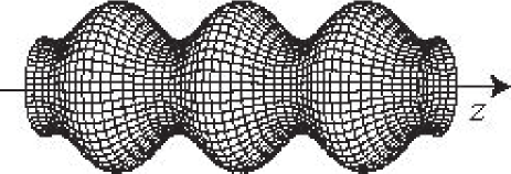
Figure 4: A sinusoidal surface defined by $r(z)=a+b\cos z$ with $a=1.5$ and $b=0.5$.

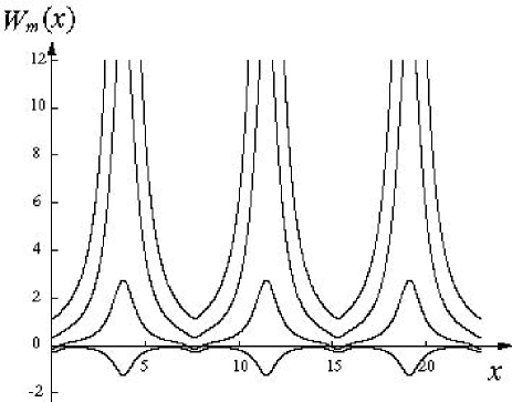
Figure 5: Effective potential energy curves $W_{m}(x)$ for the sinusoidal surface ($a=1.5$, $b=1.0$) when there is no magnetic field. These four curves corresponds to $m=0$ (bottom), $m=\pm 1$, $m=\pm 2$, and $m=\pm 3$ (top), respectively.

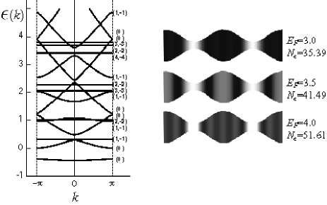
Figure 6: (left) The energy band structures for a sinusoidal surface with $a=1.5$ and $b=1.0$ without magnetic field, in which the values of $m$ corresponding to each band is shown in parenthesis. Note that for fixed $m$, energy gaps are the most prominent in a lowest part of the spectrum, and it becomes dominant for larger $m$. (right) Charge density distributions along the sinusoidal surface with three different Fermi energies $E_{F}=3.0$, $3.5$, and $4.0$, corresponding to the number of electrons per period $N_{e}=35.39$, $41.49$, and $51.61$, respectively. The brighter color corresponds to high concentration of the charge density.

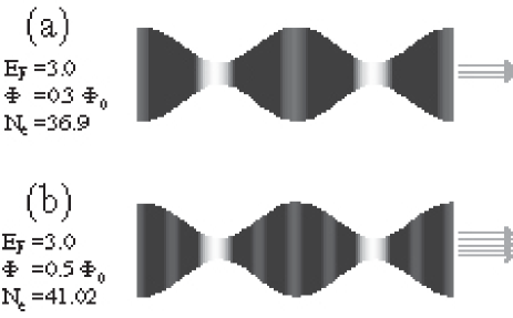
Figure 7: The charge density distribution calculated for $E_{F}=3.0$ with two different values of magnetic flux, (a) $\Phi=0.3\Phi_{0}$ and (b) $\Phi=0.5\Phi_{0}$.

V Discussions

The basic equation (Sec.II) assumes hypothetically that the surface has zero thickness and the potential energy within the surface is flat. One should bear in mind that these assumptions pose essential requirement for the scale of Fermi wavelength ($\lambda_{F}$); that is, it should be sufficiently larger than the surface thickness and the average atomic distance along the surface. This is necessary in order for the motion of an electron perpendicular to the surface to be strongly quantized and for the flat potential approximation to be valid. The condition would be satisfied if a constrained electronic system is realized using semiconductor hetero-structures ($\lambda_{F}\sim 100$nm) or bent carbon graphite sheetsVT92 ($\lambda_{F}\sim 10$nm). On the other hand, the model should be regarded as an excessive oversimplification for curved surfaces made of metallic substances, in which $\lambda_{F}\sim 0.1$nm.

Here we assume the scale of a pore diameter to be of the order of $a\sim 5$nm, which is typically the scale of pore structures in mesoporous materials and some of carbon nanotubes. Then the magnetic field should be as large as $B\sim\frac{\Phi_{0}}{a^{2}}=\frac{hc}{ea^{2}}\approx 10^{6}{\rm Gauss}=10^{2}{\rm Tesla}$ in order to make the total flux passing through the pore to be $\Phi_{0}$. This is rather large since the largest static field available is about 50 Tesla. The electronic properties could nevertheless change significantly with more moderate field strength if gap openings and/or closings may be induced by the magnetic field. It might be interesting to point out here that measurements of the Aharonov-Bohm effect in carbon nanotubes have been achieved recently. ABoscNT1 ; ABoscNT2 ; ABoscNT3

In our formulation, the initial Schr$\ddot{\rm o}$dinger equation reduces to the one-dimensional equations each of which corresponds to an angular momentum quantum number $m$ along the cylindrical axis. The effective potential energy $W_{m}(x)$ reflects the geometry of the tubule as well as the applied field, so that we may actually create a wide range of one-dimensional potentials by tuning these factors. Since the spectra for different $m$’s are independent of each other, a bound state for a $m$ can exist within the range of the essential spectrum for another $m$. We have found a simple example with this property in the case of a straight tubule with inflated part, $r(z)=a+b/(1+x^{2})$ ($a,b>0$). It is important to note that the response to a change of geometry as well as to an applied field differs among different $m$ states, while the Fermi energy can cross several partial energy spectra for different $m$’s. One may therefore pursue similar systems for applications such as electronic resonators or a selective STM probe for different $m$ states. Note that the possibility of using carbon nanotubes as STM probes has been reported. STMprobe1 ; STMprobe2

If we combine multiple tubules together, more profound and interesting effects would be expected due to the interaction between neighboring tubules. It is also interesting to study more complicated surfaces like triply periodic curved surfacesaoki which are often encountered in soft matter systems as well as mesoporous materials. In such studies, one may focus on the inherent effects of the surface metric, curvatures, symmetry and topology, where our present study may also serve as preliminary information. We may also pursue the effects of interparticle correlation, which should be essential to understand real systems.

VI Conclusions

We have formulated the problem of quantum particle motion constrained on curved tubular surfaces with cylindrical symmetry. As the surface has the continuous rotational symmetry, the two surface coordinates can be separated and the problem is finally reduced to a one-dimensional differential equation. Magnetic fields parallel to the axis is also taken into account in the formulation. Several examples are studied numerically.

Appendix A Finite difference method and boundary conditions

Using the finite difference method, the original equation (15) can be written as

$$-\frac{1}{a^{2}}y((j-1)a)+\frac{2}{a^{2}}y(ja)-\frac{1}{a^{2}}y((j+1)a)$$

$$+W(ja)y(ja)=\epsilon y(ja),$$ (30)

where $a$ is the mesh size. Several different boundary conditions have been used to obtain numerical solutions of the one-dimensional Schr$\ddot{\rm o}$dinger equation. First, the Dirichlet boundary conditions can be used for the case of non-periodic surfaces in which the effective one-dimensional potential energy $W_{m}(x)$ behaves asymptotically as $W_{m}(x)\to 0^{-}$ ($x\to\pm\infty$). The influence of the cutoff $\pm X$ of space variable $x$ becomes exponentially small for a bound state which is localized in a sufficiently smaller region than $X$, while it will decrease as $\propto 1/X$ for a scattering state. In both cases, one can estimate the energy spectrum fairly well using this boundary condition with sufficiently large $X$. If the boundary is far enough from the center, so that $|W_{m}(X)|\ll|\epsilon|$, we can improve the precision of the result by taking the Neumann boundary conditions instead. This means we assume the form $y(X+a)=y(X)e^{-\kappa a}$ for $\epsilon=-\kappa^{2}<0$ and $y(X+a)=y(X)e^{-ika}$ for $\epsilon=k^{2}>0$, where the value of $\epsilon$ should be determined self-consistently. For the case of periodic sinusoidal surfaces, we may use the usual assumption of Bloch states, which will lead to a closed form of matrix equation. This can be used to obtain the band structures.

References

- (1) H. Jensen and H. Koppe: Ann. Phys. 63 (1971) 586.
- (2) R. C. T. da Costa: Phys. Rev. A 23 (1981) 1982.
- (3) M. Ikegami and Y. Nagaoka: Prog. Theor. Phys. Suppl. 106 (1991) 235.
- (4) H. Aoki, M. Koshino, D. Takeda, H. Morise, and K. Kuroki: Phys. Rev. B 65 (2001) 035102.
- (5) Since the curvature potential at any given point is determined not only by the intrinsic curvatures but also by the extrinsic ones, the problem is essentially distinct from the classical counterpart, as discussed in Ref. 2).
- (6) R. Courant and D. Hilbert: Methods of Mathematical Physics Vol.I, Wiley-Interscience (1953).
- (7) It can be taken as the pore (inner) radius, in which case and the following equations must be scaled appropriately.
- (8) However, it seems unlikely that the potential energy is exactly solvable. See for example, L. Infeld and T. E. Hull: Rev. Mod. Phys. 23 (1951) 21.
- (9) According to a famous theorem, there exists at least one bound state if the potential energy function is always negative, and , for some fixed value of . For a presentation of the theorem, see for example, W. F. Buell and B. A. Shadwick: Am. J. Phys. 63 (1995) 256.
- (10) Hypothetical curved nanostructures made of bent graphite sheets are demonstrated in H. Terrones and M. Terrones: New Journal of Physics 5 (2003) 126.
- (11) U. C. Coskun, T.-C. Wei, S. Vishveshwara, P. M. Goldbart, and A. Bezryadin: Science 304 (2004) 1132.
- (12) S. Zaric, G. N. Ostojic, J. Kono, J. Shaver, V. C. Moore, M. S. Strano, R. H. Hauge, R. E. Smalley, and X. Wei: Science 304 (2004) 1129.
- (13) E. D. Minot, Y. Yaish, V. Sazonova, and P. L. McEuen: Nature 428 (2004) 536.
- (14) S. S. Wong, E. Joselevich, A. T. Woolley, C. L. Cheung, C. M. Lieber: Nature 394 (1998) 52.
- (15) J. H. Hafner, C. L. Cheung, C. M. Lieber: Nature 398 (1999) 761.