The twilight zone in the parametric evolution of eigenstates: beyond perturbation theory and semiclassics

Abstract

Considering a quantized chaotic system, we analyze the evolution of its eigenstates as a result of varying a control parameter. As the induced perturbation becomes larger, there is a crossover from a perturbative to a non-perturbative regime, which is reflected in the structural changes of the local density of states. For the first time the full scenario is explored for a physical system: an Aharonov-Bohm cylindrical billiard. As we vary the magnetic flux, we discover an intermediate twilight regime where perturbative and semiclassical features co-exist. This is in contrast with the simple crossover from a Lorentzian to a semicircle line-shape which is found in random-matrix models.

The analysis of the evolution of eigenvalues and of the structural changes that the corresponding eigenstates of a chaotic system exhibit as one varies a parameter $\phi$ of the Hamiltonian ${\cal H}(\phi)$ has sparked a great deal of research activity for many years. Physically the change of $\phi$ may represent the effect of some externally controlled field (like electric field, magnetic flux, gate voltage) or a change of an effective-interaction (as in molecular dynamics). Thus, these studies are relevant for diverse areas of physics ranging from nuclear HZB95 ; W55 and atomic physics TAA95 ; FGGP99 to quantum chaos W88 ; CK01 ; MLI04 ; B03 and mesoscopics VLG02 ; TA93 .

Up to now the majority of this research activity was focused on the study of eigenvalues, where a good understanding has been achieved, while much less is known about eigenstates. The pioneering work in this field has been done by Wigner W55 , who studied the parametric evolution of eigenstates of a simplified Random Matrix Theory (RMT) model of the type ${\cal H}=\bm{E}+\phi\bm{B}$. The elements of the diagonal matrix $\bm{E}$ are the ordered energies $\{E_{n}\}$, with mean level spacing $\Delta$, while $\bm{B}$ is a banded random matrix. Wigner found that as the parameter $\phi$ increases the eigenstates undergoes a transition from a perturbative Lorentzian-type line shape to a non-perturbative semicircle line-shape.

For many years the study of parametric evolution for canonically quantized systems was restricted to the exploration of the crossover from integrability to chaos MLI04 ; B03 . Only later CK01 it has been realized that a theory is lacking for systems that are chaotic to begin with. Inspired by Wigner theory, the natural prediction was that the local density of states (LDOS) should exhibit a crossover from a regime where a perturbative treatment is applicable, to a regime where semiclassical approximation is valid. However, despite a considerable amount of numerical efforts CK01 , there was no clear-cut demonstration of this crossover. Neither a theory has been developed describing how the transition from the perturbative to the non-perturbative regime takes place.

It is the purpose of this Letter to present, for the first time, a complete scenario of parametric evolution, in case of a physical system that exhibits hard chaos. We explore the validity of perturbation theory and semiclassics, and we discover the appearance of an intermediate regime (“twilight zone”) where both perturbative and semiclassical features co-exist. Without loss of generality we consider as an example a billiard system whose classical dynamics is characterized by a correlation time $\tau_{\mbox{\tiny cl}}$, which is simply the ballistic time. Associated with $\tau_{\mbox{\tiny cl}}$ is the energy scale $\hbar/\tau_{\mbox{\tiny cl}}$. Next we look on a similar billiard, but with a rough boundary. This roughness is characterized by a length scale which is $\ell$ times smaller, hence we can associate with it an energy scale $\delta E_{\mbox{\tiny NU}}=(\hbar/\tau_{\mbox{\tiny cl}})\times\ell$. The roughness does not affect the chaoticity: the correlation time $\tau_{\mbox{\tiny cl}}$ as well as the whole power spectrum are barely affected. Consequently we explain that $\delta E_{\mbox{\tiny NU}}$ is not reflected in the RMT modeling of the Hamiltonian. Still in the LDOS analysis we find that non-universal (system specific) features appear. The appearance of such features is a generic phenomenon in quantum chaos studies. It introduces a new ingredient into the theory of parametric evolution which goes beyond RMT.

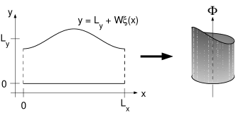
Figure 1: Left: 2D billiard with $\ell=1$. Right: Corresponding Aharonov-Bohm cylinder.

The model that we will use in our analysis is a particle confined to an Aharonov-Bohm (AB) cylindrical billiard (see Fig.1) where one can control the magnetic flux $\Phi$. The cylindrical billiard is constructed by wrapping a 2D billiard with hard wall boundaries. The lower boundary at $y=0$ is flat, while the upper boundary $y=L_{y}+W\xi(x)$ is deformed. The deformation is described by $\xi(x)=\sum_{n=1}^{\ell}A_{n}\cos(nx)$ where $A_{n}$ are random numbers in the range [-1,1]. The illustration in Fig.1 assumes a smooth boundary ($\ell=1$). The Hamiltonian of a particle in the cylindrical AB billiard is

$${\cal H}(\phi)=\frac{1}{2\mathsf{m}}\left[\left(p_{x}-\frac{e}{L_{x}}\Phi\right)^{2}+p_{y}^{2}\right]$$ (1)

supplemented by $L_{x}$ periodic boundary conditions in the horizontal direction, and hard wall boundary conditions along the lower and upper boundaries. $p_{x}$ and $p_{y}$ are the momenta. Later we shall use the notation $\phi=e\Phi/\hbar$. We consider the chaotic ${\cal H}(\phi=0)$ as the unperturbed Hamiltonian.

After conformal transformation MLI04 the billiard is mapped into a rectangular, with a mass tensor which is space dependent. Then it is possible to compute the matrix representation of the Hamiltonian in the plane wave basis $|\nu\mu\rangle$ of the rectangular. The result is:

$${\cal H}_{\nu\mu,\nu^{\prime}\mu^{\prime}}(\phi)=\frac{\hbar^{2}}{2\pi\mathsf{m}}\left\{\pi\left(\nu-\frac{\phi}{2\pi}\right)^{2}\delta_{\nu,\nu^{\prime}}\delta_{\mu,\mu^{\prime}}\right.$$

$$+\left[\frac{\mu^{2}}{8\alpha^{2}}J^{(0,2)}_{\nu^{\prime}\nu}+\epsilon^{2}J^{(2,2)}_{\nu^{\prime}\nu}(\frac{1}{8}{+}\frac{\pi^{2}\mu^{2}}{6})\right]\delta_{\mu,\mu^{\prime}}+(-1)^{\mu{+}\mu^{\prime}}\mu\mu^{\prime}$$

$$\times\left.\left[\epsilon^{2}\frac{2(\mu^{2}+\mu^{\prime 2})}{(\mu^{2}-\mu^{\prime 2})^{2}}J^{(2,2)}_{\nu^{\prime}\nu}-i\epsilon\frac{\nu+\nu^{\prime}-\phi/\pi}{\mu^{2}-\mu^{\prime 2}}J^{(1,1)}_{\nu^{\prime}\nu}\right]\right\}$$ (2)

where

$$J^{(l,k)}_{\nu^{\prime}\nu}=\int^{L_{x}}_{0}dx\,\mbox{e}^{i(\nu^{\prime}-\nu)2\pi x/L_{x}}\left(\frac{d\xi}{dx}\right)^{l}\frac{1}{(1+\epsilon\xi(x))^{k}}$$

The classical dimensionless parameters of the model are the aspect ratio $\alpha=L_{y}/L_{x}$, the tilt relative amplitude $\epsilon=W/L_{y}$, and the roughness parameter $\ell$. Upon quantization we have $\hbar$ that together with $\mathsf{m}$ and $E$ determines the De-Broglie wavelength of the particle, and hence leads to an additional dimensionless parameter $n_{E}=[L_{x}L_{y}/(2\pi\hbar^{2})]\mathsf{m}E$. For 2D billiards the mean level spacing $\Delta$ is constant, and hence $n_{E}=E/\Delta\propto 1/\hbar^{2}$ can be interpreted as either the scaled energy or as the level index. Optionally we define a semiclassical parameter $\hbar_{\mbox{\tiny scaled}}=1/\sqrt{n_{E}}$.

In the numerical study we have taken $\epsilon{=}0.06$ and $\alpha{=}1$, for which the classical dynamics is completely chaotic (for any $\phi$). We consider either $\ell{=}1$ for smooth boundary, or $\ell{=}100$ for rough boundary. The eigenstates $|n(\phi)\rangle$ of the Hamiltonian ${\cal H}(\phi)$ were found numerically for various values of the flux ($0.0006<\phi<60$). We were interested in the states within an energy window $\delta E{\approx}45$ that contains $\delta n_{E}{\sim}200$ levels around the energy $E{\approx}400$. Note that the size of the energy window is classically small ($\delta E\ll E$), but quantum mechanically large ($\delta E\gg\Delta$).

The object of our interest are the overlaps of the eigenstates $|n(\phi)\rangle$ with a given eigenstate $|m(0)\rangle$ of the unperturbed Hamiltonian:

$$P(n|m)=|\langle n(\phi)|m(0)\rangle|^{2}=\int\frac{dxdydp_{x}dp_{y}}{(2\pi\hbar)^{2}}\rho^{(n)}\rho^{(m)}$$ (3)

The overlaps $P(n|m)$ can be regarded as a distribution with respect to $n$. Up to some trivial scaling it is essentially the local density of states (LDOS). The associated dispersion is defined as $\delta E=[\sum P(n|m)(E_{n}-E_{m})^{2}]^{1/2}$ In practice we plot $P(n|m)$ as a function of $r=n-m$ or as a function of $(E_{n}{-}E_{m})$, and average over the reference state $m$. The second equality in (3) is useful for the semiclassical analysis. It involves the Wigner functions $\rho^{(n)}(x,y,p_{x},p_{y})$ which are associated with the eigenstates $|n(\phi)\rangle$. The semiclassical approximation is based on the microcanonical approximation $\rho^{(n)}\propto\delta(E_{n}{-}{\cal H}(x,y,p_{x},p_{y}))$. With this approximation the integral can be calculated analytically leading to

$$P_{\mbox{\tiny cl}}(n|m)=\frac{\Delta}{\pi\sqrt{2(\delta E_{\mbox{\tiny cl}})^{2}-\left[(E_{n}{-}E_{m})-\delta E_{\mbox{\tiny cl}}^{2}/(2E_{m})\right]^{2}}}$$ (4)

where $\delta E_{\mbox{\tiny cl}}=(\hbar v_{E}/L_{x})\phi$ with $v_{E}=(2E/\mathsf{m})^{1/2}$. It is implicit in (4) that $P_{\mbox{\tiny cl}}(n|m){=}0$ outside of the allowed range, which is where the expression under the square root is negative: For large $|E_{n}{-}E_{m}|$ there is no intersection of the corresponding energy surfaces, and hence no classical overlap.

A few words are in order regarding quantum to classical correspondence (QCC). Whenever $P(n|m)\approx P_{\mbox{\tiny cl}}(n|m)$ we call it “detailed QCC”, while $\delta E\approx\delta E_{\mbox{\tiny cl}}$ is referred to as “restricted QCC” CK01 . It is remarkable that (the robust) restricted QCC holds even if (the fragile) detailed QCC fails completely. We have verified MCK04 that also in the present system $\delta E$ is numerically indistinguishable from $\delta E_{\mbox{\tiny cl}}$.

A fixed assumption of this work is that $\phi$ is classically small. But quantum mechanically it can be either ‘small’ or ‘large’. Quantum mechanically small $\phi$ means that perturbation theory do provide a valid approximation for $P(n|m)$. What is the border between the perturbative regime and the non-perturbative regime, we discuss later. First we would like to show that the prediction which is based on perturbation theory, to be denoted as $P_{\mbox{\tiny prt}}(n|m)$, is very different from the semiclassical approximation.

In order to write the expression for $P_{\mbox{\tiny prt}}(n|m)$ we have first to clarify how to apply perturbation theory in the context of the present model. To this end, we write the perturbed Hamiltonian ${\cal H}(\phi)$ in the basis of ${\cal H}(\phi=0)$. Since we assume that the perturbation is classically small, it follows that we can linearize the Hamiltonian with respect to $\phi$. Consequently the perturbed Hamiltonian is written as ${\cal H}=\bm{E}+\phi\bm{B}$, where $\bm{E}=\mbox{diag}\{E_{n}\}$ is a diagonal matrix, while $\bm{B}=\{-(\hbar/e){\cal I}_{nm}\}$. The current operator is conventionally defined as

$${\cal I}\equiv-{\partial{\cal H}/\partial\Phi}=(e/(\mathsf{m}L_{x}))p_{x}$$

Its matrix elements can be found using a semiclassical recipe FP86 , namely $|{\cal I}_{nm}|^{2}\approx(\Delta/(2\pi\hbar))\tilde{C}((E_{n}{-}E_{m})/\hbar)$, where $\tilde{C}(\omega)$ is the Fourier transform of the current-current correlation function $C(\tau)$. Conventional condensed matter calculations are done for disordered rings where one assumes $C(\tau)$ to be exponential, with time constant $\tau_{\mbox{\tiny cl}}$ which is essentially the ballistic time. Hence $\tilde{C}(\omega)\propto 1/(\omega^{2}+(1/\tau_{\mbox{\tiny cl}})^{2})$ is a Lorentzian. This Lorentzian approximation works well also for the chaotic ring that we consider. In fact we can do better by exploiting a relation between ${\cal I}(t)$ and the force ${\cal F}(t)=-{\dot{p}_{x}}$, leading to $\tilde{C}(\omega)=(e/(\mathsf{m}L_{x}))^{2}{\tilde{C}}_{\cal F}(\omega)/\omega^{2}$. The force ${\cal F}(t)$ is a train of spikes corresponding to collisions with the boundaries. Assuming that the collisions are uncorrelated on short times we have ${\tilde{C}}_{\cal F}(\omega)\approx(8/3\pi)\mathsf{m}^{2}v_{E}^{3}/L_{y}$, for $\omega\gg(1/\tau_{\mbox{\tiny cl}})$. This is known as the “white noise” approximation BC . We have checked the validity of this approximation in the present context by a direct numerical evaluation of ${\tilde{C}}(\omega)$, and also verified the validity of the above recipe by direct evaluation of the matrix elements of $\bm{B}$ via Eq.(2), see Fig. 2(a). The classical ${\tilde{C}}(\omega)$ was numerically evaluated by Fourier analysis of the fluctuating current $\mathcal{I}(t)$ for a very long ergodic trajectory that covers densely the whole energy surface ${\cal H}(0)=E$.

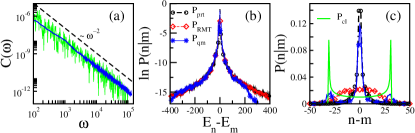
Figure 2: (a) The classical power spectrum $C(\omega)$ plotted (in grey) together with the quantum mechanical band-profile $(2\pi e^{2}/\Delta\hbar)|{\bf B}_{nm}|^{2}$ for $\ell=1$, and $\hbar_{\rm scaled}\approx 0.018$. (b) The LDOS kernel $P(n|m)$ in the perturbative regime for a billiard with $\ell=100$ and perturbation $\phi=2.7$. (c) Same as (b) but zoomed normal scale. The width of the non-perturbative component is $\Gamma/\Delta=36$. Note that in this regime the variance $\Delta E/\Delta\approx 58$ is still dominated by the (perturbative) tails. For comparison we display the calculated $P_{\mbox{\tiny prt}}$, $P_{\mbox{\tiny cl}}$, and $P_{\mbox{\tiny RMT}}$.

Perturbation theory to infinite order with the Hamiltonian ${\cal H}=\bm{E}+\phi\bm{B}$ leads to a Lorentzian-type approximation for the LDOS W55 (see also Section 18 of CK01 c). It is an approximation because all the higher orders are treated within a Markovian-like approach (by iterating the first order result) and convergence of the expansion is pre-assumed, leading to $P_{\mbox{\tiny prt}}(n|m)=\phi^{2}|\bm{B}_{nm}|^{2}/[\Gamma^{2}+(E_{n}{-}E_{m})^{2}]$. In practice the parameter $\Gamma(\phi)$ can be determined (for a given $\phi$) by imposing the requirement of having $P_{\mbox{\tiny prt}}(r)$ normalized to unity. Substituting the expression for the matrix elements we get

$$P_{\mbox{\tiny prt}}(n|m)=\frac{8\hbar^{2}(\hbar v_{E})^{3}/(3\pi\mathsf{m}L_{y}^{2}L_{x}^{3})}{(E_{n}{-}E_{m})^{2}+(\hbar/\tau_{\mbox{\tiny cl}})^{2}}\frac{\phi^{2}}{(E_{n}{-}E_{m})^{2}+\Gamma^{2}}$$ (5)

By comparing the exact $P(r)$ to the approximation Eq.(5) we can determine the regime $\phi<\phi_{\mbox{\tiny prt}}$ for which the approximation $P(r)\approx P_{\mbox{\tiny prt}}(r)$ makes sense. The practical procedure to determine $\phi_{\mbox{\tiny prt}}$ is to plot $\delta E_{\mbox{\tiny prt}}$ and to see where it departs from $\delta E_{\mbox{\tiny cl}}$. The latter is a linear function of $\phi$ while the former becomes sublinear for large enough $\phi$, (and even would exhibit saturation if we had a finite bandwidth). In case of Eq.(5) this reasoning leads to a crossover when ${\delta E_{\mbox{\tiny cl}}(\phi)\sim\hbar/\tau_{\mbox{\tiny cl}}}$. Hence we get that the border of the perturbative regime (see footnote ) is ${\phi_{\mbox{\tiny prt}}=L_{x}/(v_{E}\tau_{\mbox{\tiny cl}})\sim 1}$.

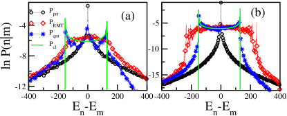
Figure 3: (a) The LDOS kernel $P(n|m)$ for $\phi=31.4$, where $\ell=100$. (b) The same parameters but $\ell=1$. In panel (a) we observe co-existence of perturbative and SC structures while in panel (b) we witness detailed QCC.

What happens to $P(r)$ in practice? If we take the Wigner RMT model as an inspiration, we expect to have at $\phi\sim\phi_{\mbox{\tiny prt}}$ a simple crossover from a $P_{\mbox{\tiny prt}}$ line-shape to a $P_{\mbox{\tiny cl}}$ line-shape. The latter is regarded as the semiclassical analogue of the (artificial) semicircle line shape. Indeed for the smooth billiard ($\ell=1$) we have verified that this naive expectation is realized MCK04 . But for the rough billiard ($\ell=100$) we witness a more complicated scenario. In Fig. 2(b,c) we show the LDOS for $\phi<\phi_{\mbox{\tiny prt}}$, where it (still) agrees quite well with $P_{\mbox{\tiny prt}}$. In Fig. 3 we show the LDOS for $\phi>\phi_{\mbox{\tiny prt}}$, where we would naively expect agreement with $P_{\mbox{\tiny cl}}$. Rather we witness a three peak structure, where the $r\sim 0$ peak is of perturbative nature, while the other are the fingerprint of semiclassics. For sake of comparison we show the corresponding results for a smooth billiard ($\ell=1$) and otherwise the same parameters. There we have detailed QCC as is naively expected. The co-existence of perturbative and semiclassical features persists within an intermediate regime of $\phi$ values, to which we refer as the “twilight zone”.

Before we adopt a phase space picture in order to explain the above observations, we would like to verify that indeed random matrix modeling does not lead to a similar effect: After all the standard Wigner model, that gives rise to a simple crossover from a Lorentzian to a semicircle line shape, assumes a simple banded matrix, which is not the case in our model. As argued above the matrix elements of $\bm{B}$ decay as $1/|n-m|^{2}$ from the diagonal. This implies that $P_{\mbox{\tiny prt}}(r)$ is in fact not a Lorentzian, and also may imply that the crossover to the non-perturbative regime is more complicated. In order to resolve this subtlety we have taken a randomized version of the Hamiltonian ${\cal H}=\bm{E}+\phi\bm{B}$. Namely, we have randomized the signs of the off-diagonal elements of the $\bm{B}$ matrix. Thus we get an RMT model with the same band profile as in the physical model. This means that $P_{\mbox{\tiny prt}}$ is the same for both models (the physical and the randomized), but still they can differ in the non-perturbative regime. Indeed, looking at the LDOS of the randomized model we observe that the semiclassical features are absent: $P_{\mbox{\tiny RMT}}(r)$ unlike $P(r)$ exhibits a simple crossover from perturbative to non-perturbative lineshape.

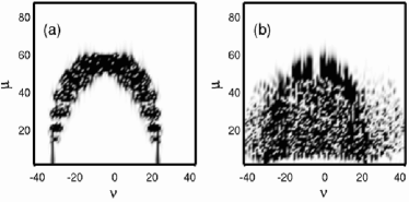
Figure 4: The probability distribution $|\langle\nu,\mu|n\rangle|^{2}$ for (a) The $n=2423$ eigenstate of the smooth ($\ell=1$) billiard; (b) The $n=1000$ eigenstate of the rough ($\ell=100$) billiard. Note that this is essentially the $(p_{x},p_{y})$ momentum distribution. The state in panel (a), unlike the state in panel (b), is a typical semiclassical state. Namely it is well concentrated on the energy shell.

In what follows we would like to argue that the structure of $P(r)$, both perturbative and non-perturbative components, can be explained using a phase space picture. [For phrasing purpose we find the “Wigner function language” most convenient, still the reader should notice that we do not need or use this representation in practice]. We recall the $P(n|m)$ is determined by the overlap of two Wigner functions. In the present context the Wigner functions $\rho^{(n)}$ are supported by shifted circles $(p_{x}-(\phi/(2\pi))^{2}+p_{y}^{2}=2\mathsf{m}E_{n}$. We are looking for their overlap with a reference Wigner function which is supported by the circle $p_{x}^{2}+p_{y}^{2}=2\mathsf{m}E_{m}$. The question is whether the overlaps of the Wigner functions $\rho^{(n)}$ and $\rho^{(m)}$ can be approximated by a classical calculation, and under what circumstances we need perturbation theory.

Generically the Wigner function has a transverse Airy-type structure. If the “thickness” of the Wigner function is much smaller compared with the separation $|E_{n}{-}E_{m}|$ of the energy surfaces then we can trust the semiclassical approximation. This will always be the case if $\hbar$ is small enough, or equivalently if we can make $\phi$ large enough. In such case the dominant contribution comes from the intersection of the energy surfaces, which is the phase space analogue of stationary phase approximation. The other extreme is the case where the “thickness” of Wigner function is larger compared with the separation of the energy surfaces (namely $\delta E_{\mbox{\tiny cl}}(\phi)<\hbar/\tau_{\mbox{\tiny cl}}$). Then the contribution to the overlap comes “collectively” from all the regions of the Wigner (quasi) distribution, not just from the intersections. In such case we expect perturbation theory to work.

The above reasoning assumes that the wavefunction is concentrated in an ergodic-like fashion in the vicinity of the energy surface. This is known as “Berry conjecture” berry . In case of billiards it implies that the wavefunction looks like a random superposition of plane waves with $|p|=(2\mathsf{m}E)^{1/2}$. We find (see Fig. 4) that this does not hold in case of a rough billiard (unless $\hbar$ were extremely small, so as to make the De-Broglie wavelength very short). Namely, in the case of a rough billiard there are eigenstates that have a lot of weight in the region $|p|<(2\mathsf{m}E)^{1/2}$. Consequently there are both semiclassical and non-semiclassical overlaps. Specifically, if we have non-semiclassical wavefunctions, and $|E_{n}-E_{m}|\sim 0$, then the collective contribution dominates, which give rise to the perturbative-like peak in the LDOS.

Our findings apply to systems, such as the rough billiard, where there is an additional (large) non-universal energy scale $\delta E_{\mbox{\tiny NU}}$. This is defined as an energy scale which is not related to the bandprofile, and hence does not emerge in the RMT modeling. Hence in general there is a distinct twilight regime $\hbar/\tau_{\mbox{\tiny cl}}<\delta E_{\mbox{\tiny cl}}(\phi)<\delta E_{\mbox{\tiny NU}}$, which is neither “perturbative” nor “semiclassical”. [In our numerics $\ell{=}100$ is so large that $\delta E_{\mbox{\tiny NU}}{\sim}E$.]

Summary: We have analyzed the parametric evolution of the eigenstates of an Aharonov-Bohm cylindrical billiard, as the flux is changed. For the first time the full crossover from the perturbative to the non-perturbative regime is demonstrated. Random matrix theory suggests a simple crossover. Instead, we discover an intermediate twilight regime where perturbative and semiclassical features co-exist. This can be understood by adopting a phase space picture, and taking into account the inapplicability of the Berry conjecture regarding the semiclassical structure of the wavefunctions.

This research was supported by a grant from the GIF, the German-Israeli Foundation for Scientific Research and Development, and by the Israel Science Foundation (grant No.11/02).

References

- (1) V. K. B. Kota, Phys. Rep. 347, 223 (2001); V. Zelevinsky et al., Phys. Rep. 276, 85 (1996).
- (2) E. Wigner, Ann. Math. 62, 548 (1955); 65, 203 (1957).
- (3) N. Taniguchi, A. V. Andreev and B. L. Altshuler, Europhys. Lett. 29, 515 (1995).
- (4) L. Kaplan and T. Papenbrock, Phys. Rev. Lett. 84, 4553 (2000); V. V. Flambaum, A. A. Gribakina, G. F. Gribakin, M. G. Kozlov, Phys. Rev. A 50, 267 (1994).
- (5) M. Wilkinson, J. Phys. A 21, 4021 (1988); O. Agam, A. V. Andreev and B. L. Altshuler, Phys. Rev. Lett. 75, 4389 (1995).
- (6) D. Cohen and T. Kottos, Phys. Rev. E 63, 036203 (2001); D. Cohen and E. J. Heller, Phys. Rev. Lett. 84, 2841 (2000); D. Cohen, Ann. Phys. 283, 175-231 (2000).
- (7) J. A. Méndez-Bermúdez, G. A. Luna-Acosta, and F. M. Izrailev, Physica E 22, 881 (2004); Phys. Rev. E 68, 066201 (2003).
- (8) L. Benet et al., J. Phys. A: Math. Gen. 36, 1289 (2003); L. Benet et al. Phys. Lett. A 277, 87 (2000); F. Borgonovi, I. Guarneri, F. M. Izrailev, Phys. Rev. E 57, 5291 (1998).
- (9) R. O. Vallejos, C. H. Lewenkopf, and Y. Gefen, Phys. Rev. B 65, 085309 (2002); G. Murthy, et al., ibid, 69, 075321 (2004); L G. G. V. Dias da Silva, et al., ibid, 69, 075311 (2004).
- (10) N. Taniguchi and B. L. Altshuler, Phys. Rev. Lett. 71, 4031 (1993); B. L. Altshuler and B. Simons, Phys. Rev. B 48, 5422 (1993).
- (11) M. Feingold and A. Peres, Phys. Rev. A 34 591, (1986); M. Feingold, D. Leitner, M. Wilkinson, Phys. Rev. Lett. 66, 986 (1991).
- (12) A. Barnett, D. Cohen and E.J. Heller, Phys. Rev. Lett. 85, 1412 (2000); J. Phys. A 34, 413 (2001).
- (13) J. A. Méndez-Bermúdez, D. Cohen and T. Kottos, in preparation (2005).
- (14) M. V. Berry, J. Phys. A 10, 2081 (1977).