Spatial correlation functions in $3-d$ Ising spin glasses

Abstract

We investigate spin-spin correlation functions in the low temperature phase of spin-glasses. Using the replica field theory formalism, we examine in detail their infrared (long distance) behavior. In particular we identify a longitudinal mode that behaves as massive at intermediate length scales (near-infrared region). These issues are then addressed by numerical simulation; the analysis of our data is compatible with the prediction that the longitudinal mode appears as massive, i.e., that it undergoes an exponential decay, for distances smaller than an appropriate correlation length.

I Motivations

Although spin glasses have been studied for over two decades, many fundamental aspects of these systems MezardParisi87b ; Young98 remain unclear. In fact, some of the most basic questions relating to their equilibrium properties remain open. Roughly, there are two schools of thought about spin-glass theories. In the droplet/scaling picture BrayMoore86 ; FisherHuse86 , at low temperature $T$ there are just two equilibrium pure phases, related by the up-down symmetry; there is no replica symmetry breaking (RSB) and connected correlation functions decay to zero at long distance. On the contrary, in the mean-field picture Parisi79 ; Parisi79b ; Parisi80 ; Parisi80b ; MezardParisi87b , at low $T$ there are many pure states that are not related by the up-down symmetry; because of this, generic connected correlation functions do not decay to zero at large distances.

Much of the theoretical and numerical work on the low temperature phase of spin glasses has been focused on the presence or absence of replica symmetry breaking. The study of correlation functions has not been pushed as much: at best, one of the spin-spin correlation functions has been measured MarinariParisi98 and was found to decrease with a power law. Nevertheless, there are a number of different theoretical predictions. Within the scaling and droplet pictures BrayMoore86 ; FisherHuse86 ; FisherHuse88 , 2-spin connected correlation functions generically decay to zero as $r^{-\theta}$, where $r$ is the distance between the spins and $\nu\equiv-1/\theta$ is the usual thermal exponent. For large dimensions $d$ one has $\theta\approx\frac{d-1}{2}$ and numerical studies indicate that $\theta(d=3)\approx 0.20$.

The predictions of the mean-field picture have been more difficult to obtain: it is necessary to go beyond the Sherrington-Kirkpatrick SherringtonKirkpatrick75 model because in that system one cannot define distances. Generally one does this using replica field theory which allows computations DominicisKondor97 in dimensions $d>6$. Note that this approach automatically forces one to consider disorder-averaged quantities. Within this formalism, one finds that $2$-spin connected correlation functions do not go to zero at large distances (because of RSB) and that the large $r$ behavior is of the form $A+B\ r^{3-d}$.

In this work we reconsider these issues theoretically and numerically in $d=3$. From replica field theory, we find the remarkable property that a certain linear combination of correlation functions decays to zero at large distance; furthermore, this decay is “fast” in an intermediate region, as corroborated by our numerical measurements.

The outline of this paper is as follows. In Section II we specify our model and we define the correlation functions that we investigate. In Section III we discuss the replica field theory approach and we compute the correlation functions of interest in the tree approximation (no loops). We then move on to the numerical simulations. The corresponding methods are presented in Section IV while results are presented in Section V. We end with our conclusions.

II General Framework

II.1 The Model

At a microscopic level, we consider a $d$-dimensional lattice of Ising spins, $S_{i}=\pm 1$, coupled by nearest-neighbor interactions. The corresponding Hamiltonian is

$$H_{J}\equiv-\sum_{\langle ij\rangle}J_{ij}S_{i}S_{j}-B\sum_{i}S_{i}\ ,$$ (1)

where we have introduced an external magnetic field $B$. Ferromagnetic couplings correspond to $J_{ij}>0$, anti-ferromagnetic ones to $J_{ij}<0$. These couplings are quenched independent random variables symmetrically distributed around $0$. To simplify the analytic part of our study, it is most appropriate to take them to be Gaussian of zero mean, while for our $d=3$ numerical study, we use $J_{ij}=\pm 1$ for simulational reasons (the difference is irrelevant in the temperature region we explore).

All the issues we consider in the following concern temperatures $T$ low enough so that one is within the frozen spin-glass phase. Furthermore, we shall always take the $B\to 0$ limit. Within the scaling/droplet picture, this limit leaves one with a single equilibrium phase; on the contrary, in the mean-field picture, $B\to 0$ simply selects one partner for each pair of $B=0$ equilibrium phases (because of RSB, there is an infinite number of these pairs).

II.2 2-Spin Correlation Functions

For any given sample, consider the standard spin-spin connected correlation function:

$$\langle S_{i}S_{j}\rangle-\langle S_{i}\rangle\langle S_{j}\rangle\ .$$

This quantity is not gauge invariant: it depends on the (arbitrary) choices of $z$ axis orientations at sites $i$ and $j$. To restore gauge invariance, one should consider either the square of this correlation function

$$\Gamma_{1}(i,j)=[\langle S_{i}S_{j}\rangle-\langle S_{i}\rangle\langle S_{j}\rangle]^{2}\ ,$$ (2)

or the difference of the squares,

$$\Gamma_{2}(i,j)=\langle S_{i}S_{j}\rangle^{2}-\langle S_{i}\rangle^{2}\langle S_{j}\rangle^{2}\ .$$ (3)

In all these quantities, $\langle\cdot\rangle$ refers to the (thermal) ensemble average with respect to the usual Boltzmann measure. If $B=0$, by symmetry we have $\langle S_{i}\rangle=0$; that is why we have introduced the infinitesimal magnetic field. Note that $\langle\cdot\rangle$ does not correspond to an average inside a pure state; $\langle S_{i}\rangle^{2}$ is thus not the Edwards-Anderson EdwardsAnderson75 order parameter.

In our study, we focus on disorder averages, averaging our observables over samples where the couplings $J_{ij}$ are randomly chosen with their a-priori distribution. We thus define

$$G_{1}(i,j)\equiv\overline{\Gamma_{1}(i,j)}\ \ \ G_{2}(i,j)\equiv\overline{\Gamma_{2}(i,j)}\ ,$$ (4)

where the overline denotes this disorder average.

What do we expect for these quantities? Clearly, in the droplet/scaling picture, the limit $B\to 0$ leads to a single pure phase and so connected correlation functions go to zero. Furthermore, the large distance behavior is controlled by a zero temperature disordered fixed point. Roughly, this leads to effective couplings of “block” spins at large scales that have a broad distribution: typical values scale as $r^{\theta}$ for blocks at distance $r$. Since this distribution is bell shaped with a non-zero value at the origin, droplets of characteristic scale $r$ are thermally excited with a probability going as $kTr^{-\theta}$. This feature leads to connected correlation functions decaying as $r^{-\theta}$.

In the mean-field picture the low $T$ phase undergoes RSB: connected correlation functions do not go to zero at large $r$. Interestingly, the $r\to\infty$ limit of the disorder averaged $\langle S_{i}S_{j}\rangle^{2}$ can be expressed simply in terms of a moment of configurational overlaps. One defines the spin overlap $q$ of two configurations $(1)$ and $(2)$ as

$$q^{(1,2)}\equiv\frac{\sum_{i}S_{i}^{(1)}S_{i}^{(2)}}{N}\ ,$$ (5)

where $N$ is the total number of spins. A straightforward computation of $\overline{\langle q^{2}\rangle}$ gives

$$\overline{\langle q^{2}\rangle}=\frac{\sum_{ij}\overline{\langle S_{i}S_{j}\rangle^{2}}}{N^{2}}$$ (6)

The large volume limit of this quantity can be obtained by replacing the correlation functions on the right hand side by their long distance limit: in this way one sees that the long distance limit of the first contribution to $G_{2}$ is $\overline{\langle q^{2}\rangle}$. As we shall see later, the mean-field formalism also predicts a very non-trivial relation between the limiting values of $G_{1}$, $G_{2}$ and a certain combination of moments of overlaps.

A more subtle question for the mean-field picture is how the correlation functions approach their large $r$ limits. The framework for addressing this question is replica field theory, which leads to the conclusion DominicisKondor97 that the decay should follow a power law in $r$. Our goal here is to reconsider that computation, focusing in particular on linear combinations of $G_{1}$ and $G_{2}$.

III Replica Field Theory for Generalized Correlation Functions

III.1 Starting Point

We consider the linear combination of correlation functions $\alpha G_{1}+(1-\alpha)G_{2}$ which can be written as

$$\chi^{\alpha}(i,j) = \overline{\langle S_{i}S_{j}\rangle^{2}}-2\alpha\overline{\langle S_{i}S_{j}\rangle\langle S_{i}\rangle\langle S_{j}\rangle}$$ (7)

$$+ (2\alpha-1)\overline{\langle S_{i}\rangle^{2}\langle S_{j}\rangle^{2}}\ ,$$

where $\alpha$ is a parameter that can take real values. The brackets indicate thermodynamical averages in the presence of the infinitesimal magnetic field, while the overline indicates an average over the disorder distribution. In the case $\alpha=1$, after summing over $j$, we obtain the usual expression for the spin-glass susceptibility $\chi$.

The starting point of replica field theory is the (truncated) effective Lagrangian describing the replicated theory DominicisKondor97

$${\cal L} \equiv -\frac{1}{4}\sum_{a,b}\sum_{\bf p}(p^{2}-2\tau)\Phi^{ab}({\bf p})\Phi^{ab}({\bf-p})$$

$$+ \frac{w}{6\sqrt{N}}\sum_{a,b,c}\sum_{\bf\{p_{i}\}}\Phi^{ab}({\bf p_{1}})\Phi^{bc}({\bf p_{2}})\Phi^{ca}({\bf p_{3}})$$

$$+ \frac{u}{12N}\sum_{a,b}\sum_{\bf\{p_{i}\}}\Phi^{ab}({\bf p_{1}})\Phi^{ab}({\bf p_{2}})\Phi^{ab}({\bf p_{3}})\Phi^{ab}({\bf p_{4}})\ ,$$

where all the sums over momenta are constrained in such a way that the total momentum adds to zero. Note that to reduce the complexity of the presentation, we have used discrete sums over momenta rather than the integrals that arise in the thermodynamic limit, $N\to\infty$. Expanding around the mean-field solution

$$\Phi^{ab}({\bf p})=\delta_{{\bf p},0}\ q_{ab}+\phi^{ab}({\bf p})\ ,$$ (9)

one finds

$${\cal L} = {\cal L}_{mf}(q)-\frac{1}{2}\sum_{a<b,c<d}\sum_{\bf p}\phi^{ab}({\bf p})M^{ab;cd}({\bf p})\ \phi^{cd}(-{\bf p})$$ (10)

$$+ {\cal L}_{int}(\phi)\ ,$$

where

$${\cal L}_{mf}(q)=N\{\frac{\tau}{2}\sum_{ab}q_{ab}^{2}+\frac{w}{6}\sum_{a,b,c}q_{ab}q_{bc}q_{ca}+\frac{u}{12}\sum_{a,b}q_{ab}^{4}\}\ ,$$ (11)

$M$ is the matrix of the Gaussian fluctuations and ${\cal L}_{int}$ is an interaction term including contributions up to the fourth order in $\phi$ (see Eq. (III.1)).

In the context of this replicated field theory, the spin correlation function that appears in Eq. (7) can be expressed in terms of field correlations. For example, we have

$$\overline{\langle S_{i}S_{j}\rangle^{2}}=\overline{\langle S_{i}^{(1)}S_{i}^{(2)}S_{j}^{(1)}S_{j}^{(2)}\rangle}=\langle\Phi^{12}_{i}\Phi^{12}_{j}\rangle_{\cal L}=C^{12;12}(i,j)\ ,$$ (12)

where $\langle...\rangle_{\cal L}$ is an average performed using the effective Lagrangian of Eq. (III.1) and where the superscripts on the spins are replica indices. In the low temperature phase, where one assumes that many states may exist, the expression for $\chi^{\alpha}(i,j)$ leads one to consider all the possible ways in which $4$ replica indices can appear. Then we have the following general expression (in position space, or, equivalently in momentum space):

$$\chi^{\alpha} = \frac{1}{n(n-1)}\sum_{a,b}\{C^{ab;ab}-\frac{2\alpha}{(n-2)}\sum_{c\neq b}C^{ab;ac}$$ (13)

$$+ \frac{(2\alpha-1)}{(n-2)(n-3)}\sum_{c,d\neq a,b}C^{ab;cd}\}\$$

where we have dropped the $(i,j)$ dependence of $\chi^{\alpha}$ and of the $C$s to lighten the notation.

We can now separate, as in Eq. (9), the fluctuating part from the mean-field part:

$$C^{ab;cd}(i-j) = \langle\Phi^{ab}_{i}\Phi^{cd}_{j}\rangle=q_{ab}q_{cd}+\langle\phi^{ab}_{i}\phi^{cd}_{j}\rangle$$ (14)

$$= q_{ab}q_{cd}+G^{ab;cd}(i-j)$$

$$+ {\rm loop\ \ corrections}\ ,$$

where $G=M^{-1}$ is the free propagator (see Eq. (10)), and where we schematically denote by $i-j$ the distance between $i$ and $j$. From this we get

$$\chi^{\alpha} = \chi^{\alpha}_{mf}+\chi^{\alpha}_{fl}=\frac{2-\alpha}{3n(n-1)}[\sum_{ab}q_{ab}^{2}+\sum_{abc}q_{ab}q_{ac}]$$ (15)

$$+ \frac{1}{n(n-1)}\sum_{a,b}\{G^{ab;ab}-\frac{2\alpha}{(n-2)}\sum_{c\neq b}G^{ab;ac}$$

$$+ \frac{(2\alpha-1)}{(n-2)(n-3)}\sum_{c,d\neq a,b}G^{ab;cd}\}$$

$$+ {\rm loop\ \ corrections\ .}$$

Note that in the mean-field contribution $\chi^{\alpha}_{mf}$ the sums run over all replica indices but we have included only the terms which have a finite limit when $n\to 0$.

We now compute the generalized correlation function $\chi^{\alpha}$ considering the mean-field solution together with the Gaussian fluctuations around it, disregarding the loop corrections in Eq. (15).

III.2 Mean-Field Solution and Free Propagators

The mean-field solution $q_{ab}$ is obtained by minimizing the Lagrangian ${\cal L}_{mf}$; it is thus given by the saddle point equation

$$2\tau q_{ab}+w(q^{2})_{ab}+\frac{2u}{3}q_{ab}^{3}=0\ .$$ (16)

This equation is solved using an ultrametric Ansatz for the form of the matrix $q$  Parisi79b ; Parisi80 ; Parisi80b . According to this Ansatz the matrix $q$ is hierarchically divided into blocks by means of a procedure based on $R$ steps: at each step $r$ the size of the blocks is set to $p_{r}$, with $p_{0}=n$ and $p_{R+1}=1$. If two replica indices belong to the same block of size $p_{r}$ but to two distinct blocks of size $p_{r+1}$ then $q_{ab}=q_{r}$, and we say that their “co-distance” $a\cap b$ in replica space is $r$. In this way the matrix $q$ is parameterized by the $R$-step function $q_{r}$, where $r\in[0,R]$; note that each $q_{r}$ has a multiplicity $\delta r=p_{r}-p_{r+1}$. One can also represent this procedure with blocks via a hierarchical tree, having its root at $r=0$, its leaves at $r=R$, and having $p_{r}/p_{r+1}$ branches at nodes of height $r$. Replica indices lie on the leaves and their overlap is $q_{r}$ if they join at a node of height $r$ on the tree. At the end one takes the limit $R\to\infty$ and $n\to 0$: now the values $p_{r}$ tend to a monotonic increasing function that takes values in $[0,1]$. In this limit, setting for example $p_{r}=x$ with $x\in[0,1]$, $q_{r}$ becomes a continuous function $q(x)$ and we indicate the replica co-distance as $a\cap b=x$. The well-known mean-field solution of Eq. (16) then reads:

$$q(x) = \frac{w}{2u}x\quad\quad\quad\quad x<x_{1}$$

$$q(x) = q_{1}=\frac{w}{2u}x_{1}\quad x_{1}<x<1$$

$$\rm{with}\quad\quad\tau - wq_{1}+uq_{1}^{2}=0\ .$$ (17)

To calculate the free propagator $G$, one has to evaluate the fluctuation matrix

$$M^{ab;cd}=\frac{\partial^{2}{\cal L}_{mf}(q)}{\partial q_{ab}\partial q_{cd}}$$ (18)

given the mean-field solution Eq. (17), and then invert it. To do this, it is convenient to parametrize both the fluctuation matrix $M$ and the propagator $G=M^{-1}$ in a way that exploits the ultrametric structure of the mean-field solution. Each element of $M$ and $G$ is in principle labeled by four replica indices. However, due to ultrametricity, three replica co-distances are enough to characterize the geometrical structure of the four indices. In terms of these co-distances we can then identify two possible “sectors” for the propagator $G^{ab;cd}$ (and for $M^{ab;cd}$):

• The replicon sector: when $a\cap b=c\cap d\equiv r$

  $$G^{ab;cd}=G^{r,r}_{u,v}\ ,$$ (19)

  with $u=\max(a\cap c,a\cap d)$, $v=\max(b\cap c,b\cap d)$ and $u,v>r$.

• The longitudinal-anomalous sector: when $a\cap b\equiv r$ and $c\cap d\equiv s$

  $$G^{ab;cd}=G^{r,s}_{t}\ ,$$ (20)

  with $t=\max(a\cap c,a\cap d,b\cap c,b\cap d)$.

These two sectors are illustrated in Fig. 1.

Figure 1: Topologies associated with the replicon sector (top) and the longitudinal anomalous sector (bottom).

The inversion of the fluctuation matrix is not simple DominicisKondor97 . It can be carried out using the Replica Fourier transform when $d>6$, since in this case there are no infra-red divergences (see DominicisCarlucci97 ; CarlucciThesis and the Appendix A of this paper), enabling one to block-diagonalize the fluctuation matrix. In this way the propagators $G$ are expressed in terms of Replica Fourier transformed variables, whose explicit form in terms of the mean-field solution $q_{ab}$ can be computed. In the next section we will use these expressions to compute the generalized correlation functions.

III.3 The Generalized Correlation Functions

The expression for the mean-field part $\chi^{\alpha}_{mf}$ is easily obtained using Eq. (17):

$$\chi^{\alpha}_{mf} = \frac{2-\alpha}{3}\left[\int_{0}^{1}dx\ q^{2}(x)-\left(\int_{0}^{1}dx\ q(x)\right)^{2}\right]$$ (21)

$$= \frac{2-\alpha}{3}\frac{w^{2}}{4u^{2}}\left[\frac{x_{1}^{3}}{3}-\frac{x_{1}^{4}}{4}\right]\ .$$

Note that this expression gives for $\alpha=2$ a mean-field value equal to zero. As we will discuss later, this fact is the consequence of a “sum rule”. However, as we shall see in the next sub-section, the case $\alpha=2$ is peculiar also at the level of fluctuations.

In the Parisi MezardParisi87b solution, $x(q)$, the inverse of $q(x)$, has a simple expression in terms of $P(q)$:

$$P(q)=\frac{dx(q)}{dq}\ ,$$

where

$$P(q)\equiv\overline{\left\langle\delta\left(q-\frac{1}{N}\sum_{i}S_{i}^{(1)}S_{i}^{(2)}\right)\right\rangle}\ .$$

This makes clear that

$$\chi^{\alpha}_{mf}=\frac{2-\alpha}{3}\left(\overline{\left\langle q^{2}\right\rangle}-\overline{\left\langle q\right\rangle^{2}}\right)\equiv\frac{2-\alpha}{3}\sigma_{|q|}\ .$$

Note that in the present computation the overlaps are constrained to positive values because of the infinitesimal positive magnetic field; however, that will not be case for the numerical data which were collected in zero field (see the next section). For this reason and to use a common notation throughout the paper, we indicated the variance of $q$ with respect to $P(q)$ in the presence of an infinitesimal field as $\sigma_{|q|}$.

For the fluctuating part, with the parameterization given in the previous section, and exploiting the definition of Replica Fourier transform, we obtain in the $R$-step Ansatz:

$$\chi^{\alpha}_{fl} =$$

$$- \frac{2-\alpha}{3}\left\{\sum_{0}^{R}\delta r\sum_{0}^{R}\delta s\ G^{rs}_{R+1}+\frac{1}{4}\sum_{0}^{R}\delta r\ G^{rr}_{\widehat{r+1}}\right.$$

$$+ \left.\sum_{0}^{R}\delta r\ _{R}G^{rr}_{R+1,\widehat{r+1}}+\sum_{0}^{R}\delta r\ G^{rr}_{R+1,R+1}\right\}$$

$$- \frac{2\alpha-1}{3}\left\{\sum_{0}^{R}\delta r\ G^{r,r}_{\widehat{r+1},\widehat{r+1}}+\frac{1}{2}\sum_{0}^{R}\delta r\sum_{0}^{R}\delta s\ G^{r,s}_{\hat{0}}\right\}\ ,$$

where the $\widehat{\cdots}$ indicates that we have used an operation of Replica Fourier transform with respect to the hatted variable, and ${}_{R}G^{r,r}_{u,v}$ stands for a pure replicon propagator (where the longitudinal-anomalous contribution has been taken away, see Appendix A).

III.3.1 The Special Case $\alpha=2$

In the case of $\alpha=2$ the first two lines of terms in Eq. (III.3) disappear and the calculation simplifies a lot. We start with the general expression for the replica Fourier transform of the replicon propagator (see Appendix A):

$$G^{r,r}_{\hat{k},\hat{l}}=\frac{1}{p^{2}+\frac{w^{2}}{4u}[k^{2}+l^{2}-2r^{2}]}\ ,$$ (23)

and thus the first sum gives

$$\sum_{0}^{R}\delta r\ G^{r,r}_{\widehat{r+1},\widehat{r+1}} = \sum_{0}^{R}(p_{r}-p_{r+1})\frac{1}{p^{2}}$$ (24)

$$= (p_{0}-1)\frac{1}{p^{2}}\ \ \ \mathop{\longrightarrow}_{n\to 0}\ \ \ \frac{-1~{}}{p^{2}}\ .$$

The second sum is less straightforward. When we go to the continuous limit, the variables $p_{r},p_{s}$ with $r,s\leq R$ assume values in the continuum interval $[0,x_{1}]$, while $p_{R+1}\equiv 1$; because of that, it is convenient to separate the sum into two different pieces before taking the limit of continuous replica symmetry breaking ($R\to\infty$):

$$\frac{1}{2}\sum_{0}^{R}\delta r\sum_{0}^{R}\delta s\ G^{r,s}_{\hat{0}}=\sum_{r\leq s\leq R-1}\delta r\ \delta s\ G^{r,s}_{\hat{0}}$$ (25)

$$+ (p_{R}-p_{R+1})\sum_{r\leq R-1}\delta r\ G^{r,R}_{\hat{0}}+(p_{R}-p_{R+1})^{2}\ G^{R,R}_{\hat{0}}$$

$$\longrightarrow\int_{0}^{x_{1}}dx\int_{x}^{x_{1}}dy\ G^{x,y}_{\hat{0}}$$

$$+ (1-x_{1})\int_{0}^{x_{1}}dx\ G^{x,x_{1}}_{\hat{0}}+(1-x_{1})^{2}\ G^{x_{1},x_{1}}_{\hat{0}}\ .$$

Now we can use the expression of the longitudinal Fourier transform obtained in DominicisKondor97 :

$$G^{x,y}_{\hat{0}}=\frac{2}{p^{2}\hat{p}}\ \ \frac{\sinh{\frac{x}{\hat{p}}}}{\cosh{\frac{x_{1}}{\hat{p}}+\frac{1-x_{1}}{\hat{p}}\sinh{\frac{x_{1}}{\hat{p}}}}}$$

$$\left[\cosh{\frac{x_{1}-y}{\hat{p}}}+\frac{1-x_{1}}{\hat{p}}\sinh{\frac{x_{1}-y}{\hat{p}}}\right]\ ,$$ (26)

where $\hat{p}^{2}=\frac{u}{w^{2}}\ p^{2}=\frac{x_{1}}{2wq_{1}}p^{2}$. In this way we get for Eq. (25)

$$\frac{1}{p^{2}}\left[1-{\hat{p}}\frac{\tanh{\frac{x_{1}}{\hat{p}}}+\frac{1-x_{1}}{\hat{p}}}{1+\frac{1-x_{1}}{\hat{p}}\tanh{\frac{x_{1}}{\hat{p}}}}\right]\ ,$$ (27)

and altogether we get

$$\chi_{fl}^{\alpha=2}(p)=\frac{\hat{p}}{p^{2}}\frac{\tanh{\frac{x_{1}}{\hat{p}}}+\frac{1-x_{1}}{\hat{p}}}{1+\frac{1-x_{1}}{\hat{p}}\tanh{\frac{x_{1}}{\hat{p}}}}\ .$$ (28)

Note that the singularity present in the replicon part is canceled by the $1/p^{2}$ term in the longitudinal part, leaving a less divergent quantity in the long wavelength limit. Let us now look more in details at the infrared behaviour of this correlation. In the far-infrared region, i.e., for momenta much smaller than the small mass $2x_{1}wq_{1}$ (see DominicisKondor97 ), we have that $x_{1}/{\hat{p}}\to\infty$ and

$$\chi_{fl}^{\alpha=2}(p)\simeq\frac{x_{1}}{\hat{p}}\left(\frac{p^{2}}{2x_{1}wq_{1}})\right)^{1/2}\sim\frac{1}{p}$$ (29)

$$\mathrm{for}\ \ \ p^{2}\ll 2x_{1}wq_{1}\ .$$

On the other hand, in the so called near-infrared region, i.e., in between the small mass $2x_{1}wq_{1}$ and the large mass $2wq_{1}$, we have that $x_{1}/{\hat{p}}\ll 1$ and we get

$$\chi_{fl}^{\alpha=2}(p)\simeq\frac{1}{p^{2}+2wq_{1}(1-x_{1})}$$ (30)

$${\mathrm{for}}\ \ \ 2x_{1}wq_{1}\ll p^{2}\ll 2x_{1}wq_{1}\ .$$

Thus, for intermediate momenta (or intermediate distances, i.e., between the correlation lengths associated to the two masses), $\chi^{\alpha=2}_{fl}(p)$ behaves as if it were massive. Only at very large distance does one feel the infrared singularity in $1/p$ (or the associated inverse power behaviour in distance). The width of the region where the apparent massive behaviour is felt depends on the size of $x_{1}$. For $6<d<8$, one has $x_{1}\sim(w^{2}/\zeta)\ t^{(d-6)/2}$, where $t$ is the reduced temperature $(T_{c}-T)/T_{c}$ and $\zeta$ the number of neighbours. As one reaches $d=6$ from above $x_{1}$ remains small like $w^{2}/\zeta$. Below $d=6$, $x_{1}$ is a function of $w^{2}/\zeta$ with, at the critical fixed point, $w^{2}/\zeta=\epsilon/2$, i.e., $x_{1}=f(\epsilon)\sim\epsilon/2$ for $\epsilon\ll 1$. In three dimensions we have unfortunately no explicit knowledge of the size of $x_{1}$, though the previous computation shows that, if the two mass-scales remain well separated, there exists a range of distances where massive-like behaviour occurs.

In the far-infrared region one can apply scaling rules to guess what power-law behaviour arises below $d=6$. From the Kadanoff scaling hypothesis we expect the correlation function to decay as $\chi^{\alpha=2}_{fl}(p)=\psi(p\ \xi)/p^{2-\eta}$, where $\xi\sim t^{-\nu}$ is the associated correlation length. From Eq. (III.3.1) we then get

$$\chi_{fl}^{\alpha=2}(p)\simeq\frac{x_{1}}{\hat{p}}\left(\frac{p^{2}}{2x_{1}wq_{1}}\right)^{1/2}\rightarrow\ \frac{x_{1}}{p^{2-\eta}}\left(\frac{p^{\frac{1}{\nu}}}{x_{1}t}\right)^{\beta/2}$$ (31)

that is

$$\chi_{fl}^{\alpha=2}(p)\sim\frac{x_{1}}{p^{2-\eta}}\frac{p^{\frac{d-2+\eta}{4}}}{t^{\beta}}$$ (32)

or by Fourier Transform

$$\chi_{fl}^{\alpha=2}(r)\sim\frac{1}{r^{\frac{5}{4}(d-2+\eta)}}\ .$$ (33)

Consider now instead the near-infrared regime. In this region, the generalized correlation function with $\alpha=2$ shows an exponential decay with distance, the asymptotic power law decay arising only at still much larger length scales. As we shall see, this behaviour is peculiar of $\alpha=2$. Indeed for every other value of $\alpha$ the correlation function always decays algebraically (see Sec. III.3.2). Within the framework of the scaling/droplet model BrayMoore86 ; FisherHuse86 ; FisherHuse88 correlation functions always decay algebraically, with no difference between near and far-infrared.

We note that in the near-infrared the $\alpha=2$ correlation function has a longitudinal nature in the usual field theory terminology. It is then appropriate to compare the present result with what happens in other systems where a continuous symmetry is broken. It is known that in $O(N)$ systems the longitudinal mode, which is massive at the level of Gaussian fluctuations, is converted into a massless mode when loop corrections are taken into account BrezinWallace73 ; BrezinWallace73b , and one may wonder whether the same also happens in spin glasses. The argument for the Heisenberg model, as detailed in Appendix (B), relies on the fact that the effective interaction between Goldstone modes vanishes in the infrared limit, and these modes are thus effectively free. In the Ising spin glass, however, the situation is different since in this case Goldstone modes remain coupled in the infrared DominicisKondor97 . As a consequence, the argument for the $O(N)$ case does not apply here and the longitudinal mode $\chi^{\alpha=2}$ in the near-infrared is expected to remain massive: massive-like behaviour at intermediate scales is expected to occur even if the loop corrections are included.

Finally, we note that a different behavior is found if our analysis for $d>6$ is extended to configurations which are constrained to have a fixed value of their overlaps. For example, for $r=s=0$, that is for configurations having zero mutual overlap, the longitudinal part is identically zero, and we are left with a singular $1/p^{2}$ behavior in the whole infrared region. (This happens in fact for all values of $\alpha$, not just for $\alpha=2$.)

III.3.2 The Case $\alpha\neq 2$

For $\alpha\neq 2$ a calculation similar to the one detailed in the previous section enables us to estimate the most singular contributions in the limit ${\bf p}\to 0$. We find that

$$\chi_{fl}^{\alpha\neq 2}\sim\frac{{\rm A}+\log p}{p^{3}}+\frac{\rm B}{p^{2}}\ ,$$ (34)

where $A$ and $B$ are two numerical coefficients. These expressions are valid for $d>6$. Using general scaling arguments for the integrals appearing in the calculation, at $d<6$ one can argue that Eq. (34) gives in real space

$$\chi_{fl}^{\alpha\neq 2}\sim\frac{\rm A}{r^{\frac{3}{4}(d-2+\eta)}}+\frac{\rm B}{r^{d-2+\eta}}\ ,$$ (35)

where $\eta$ is an anomalous dimension. In $d=3$, two recent numerical estimates for the $J_{ij}=\pm 1$ model give $\eta=-0.35\pm 0.05$ KawashimaYoung96 , and $\eta=-0.22\pm 0.02$ MariCampbell99 . The corresponding values for the exponent $(3/4)(d-2+\eta)$ of the leading term of Eq.(35) are, respectively, $0.49\pm 0.04$ and $0.585\pm 0.015$.

IV Computational Methods

IV.1 Monte Carlo Simulations

It is interesting to test the analytical predictions we have just provided (based on $d>6$ calculations) to what happens in a three dimensional system. This means estimating the correlation functions of Eq. (4) from numerical simulations. To do that, we have generated $512$ spin-glass samples, where the couplings $J_{ij}$ were randomly set to $\pm 1$; we considered mainly $12\times 12\times 12$ cubic lattices with periodic boundary conditions (smaller lattices have also been used, allowing us to see the qualitative behavior of finite size effects).

For each such sample we produced over $1000$ equilibrium spin configurations which were essentially independent (since they were separated by a large number of updates). This was achieved using the Parallel Tempering Monte Carlo method HukushimaNemoto96 ; ZulianiThesis as follows. The temperatures used went from $0.1$ to $2.0$ in steps of $\Delta T=0.1$ (the critical temperature $T_{c}$ in this model is about $1.1$). At each temperature we performed sweeps using the usual Metropolis algorithm and followed this by trial exchanges between neighboring temperatures; we call this sequence a pass of the algorithm. The value of $\Delta T$ was such that these exchanges succeeded with a probability close to $1/2$.

After thermalizing the system using a million such passes, we stored configurations every 1000 passes for further analysis. With these choices of parameters, we verified that the configurations kept were compatible with being statistically independent by examining their overlaps. Furthermore, we also checked that each configuration visited many times all the temperature values as suggested in Marinari98 and that the distribution of overlaps for each sample was symmetric with high accuracy. Finally, the use of bit-packing enabled us to speed up the computation (this trick is particularly useful for the case of $J_{ij}=\pm 1$ couplings). The overall computation was performed on a cluster of Linux-based PCs running at 333 MHz and represents the equivalent of $2$ years of mono-processor time.

IV.2 Configuration Space Decomposition

All of the theory exposed in Section III implies the presence of an infinitesimal magnetic field. Performing this limit numerically is a nuisance because of the necessity to have several values of the magnetic field and to control the accuracy of the limit. Fortunately, it is possible to avoid such an extrapolation by remarking that the role of a very small magnetic field is to select half of the $B=0$ configurations. The simplest implementation of this is to keep only those configurations (generated at $B=0$) whose total magnetization $M$ is positive. This should give the correct selection when the lattice size $L$ tends to $\infty$, though of course with finite $L$ this may lead to some undesirable effects. What properties does one expect in the thermodynamic limit? In the mean-field picture, there are many equilibrium states, all coming in pairs when $B=0$; if one adds an infinitesimal field, only one state in each pair survives and the overlap with the remaining states becomes positive.

In practice, we have found that the selection of those configurations with $M>0$ left us with quite a few overlaps that were negative. (This was severe for some disorder samples and less in others.) We thus sought a better decomposition of the configuration space into two parts related by the global spin flip symmetry. For each disorder sample, we used the following procedure. (A nearly identical method was applied in CilibertiMarinari04 ).

In a first iteration, we successively consider the equilibrium configurations, and flip them if their mean overlap with the previous configurations is negative. In the iterations thereafter, one repeats these flips but now using the mean overlap with all the other configurations. In other words, we try to “align” the configurations as much as possible; effectively, our procedure is a kind of descent optimization method where we seek to have all mean overlaps be positive; the first pass is useful for generating a good starting set.

In many cases, we find that this iterative procedure converges to a fixed point where all mean overlaps are positive. This procedure has then split the configuration space into two parts that are related by the global spin flip symmetry. When the algorithm does not converge, we repeat the procedure with a new first pass after permuting randomly the configurations; this can lead to convergence, but if it does not, we simply stop after some number of trials and accept an “imperfect” decomposition.

Given the set of aligned configurations (about half of them have been flipped), we can then look at individual rather than mean overlaps. The main test of whether the configuration space decomposition is “perfect” is then the positivity of all the overlaps between these aligned configurations.

IV.3 Parametrization of Correlation Functions

Within the theoretical analysis, one controls only the small momentum behavior of $\chi^{\alpha}$ (e.g., $p\to 0$ in formula (34)), that is the large distance region. There is thus some arbitrariness in the choice of fitting functions when comparing the data to the theoretical predictions. Our choice of functions is as follows. Start with a correlation function $G(p)$ on the infinite lattice that has a power law behavior $p^{-c}$ as $p\to 0$; the simplest choice is

$$G({\bf p})=\frac{1}{\left[2\sum_{\mu}(1-\cos(p_{\mu})\right]^{c/2}}$$ (36)

as motivated by the requirement that $G({\bf p})$ be periodic in the components $p_{\mu}$ of ${\bf p}$. (We work in units of the lattice spacing.) This correlation function can be used also on a finite size lattice of size $L\times L\times L$ with periodic boundary conditions as long as we take the correct discrete values of the $p_{\mu}$. We thus take this $G({\bf p})$ and Fourier transform it to coordinate space. All our measurements are for $i$ and $j$ on an axis of the lattice, and when performing the transform we must remove the ${\bf p}={0}$ contribution; this defines a function hereafter called $G_{c}(r)$. An analogous procedure was used in MarinariMonasson95 . One can also perform this computation with a mass term, leading to exponentially decaying correlation functions; we do this by adding $m^{2}$ in the denominator of the right hand side of Eq. (36) and setting $c=2$, leading to the function $G_{m}(r)$. (We performed checks on our code using the high precision values for such functions in FriedbergMartin87 .) The resulting family of functions we use for our fits are then $a+bG_{c}(r)$ and $a+bG_{m}(r)$.

V Results

V.1 Effect on Overlaps of the Decomposition

In the thermodynamic limit, we expect configuration space decomposition schemes to lead to aligned configurations for which the overlaps are positive. However, one can expect some schemes to work better than others when $L$ is relatively modest (in our case $L=12$). As we already pointed out, the simplest procedure does not work so well, so let us examine the overlaps found with our “improved” scheme previously described. For each sample, we have viewed the distribution $P(q)$ of overlaps found for each pair of configurations, both before and after the alignment. In the majority of the samples, the procedure leads to nearly all overlaps being positive; yet there are some samples for which one still has a significant number of overlaps that are negative.

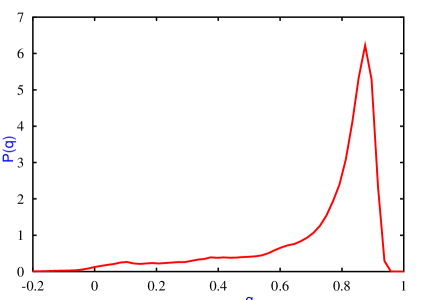
Figure 2: Example of distribution of overlaps for a disorder sample after the configuration space decomposition. $T=0.5$.

In Fig. 2 we show an example where a rather small fraction of the overlaps are negative. When considering all 512 of our samples, the decomposition is reasonably good but not perfect; this is not surprising considering our lattice size ($L=12$). Because of these effects, we expect our analysis of correlation functions to suffer from small systematic effects since quantities such as $\langle S_{i}\rangle$ are probably estimated with a residual bias.

V.2 Correlation Functions

Now we confront the different predictions of the replica field theory approach to the properties of the system as extracted from our simulations.

The first important prediction of replica field theory is that the large distance limit of $\chi^{\alpha}$ is $(2-\alpha)/3$ times the variance of $q$ in the presence of an infinitesimal magnetic field. This prediction arises from the mean-field computation; it continues to hold when taking into account the Gaussian fluctuations; furthermore, as argued in the previous section, it should continue to hold within the loop expansion.

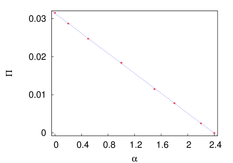
Figure 3: Large distance value $\Pi$ of the correlation function $\chi^{\alpha}$ of Eq. (7) as a function of $\alpha$. Theoretically, the change of sign should be at $\alpha=2$. (The data are for $T=0.5$.)

We have fitted $\chi^{\alpha}(i,j)$ using the class of functions $a+bG_{c}(r)$ and $a+bG_{m}(r)$ defined before. We find that for $\alpha$ not close to $2$ the power fit is far superior and gives a good value for $\chi^{2}$: there is at least one order of magnitude difference between the power law best fit $\chi^{2}$ and the exponential best fit $\chi^{2}$. On the contrary, when $\alpha\approx 2$, the exponential fit is better: in this case the decay is indeed so fast that only at distance $1$ do we get sometimes a signal significantly different from zero over the plateau value.

The constant value obtained from these fits gives the long distance limit of $\chi^{\alpha}$; for $T=0.5$, we plot in Fig. 3 these limits as a function of $\alpha$. The behavior is linear in $\alpha$ as it should, and the values change sign not far from $\alpha=2$. Furthermore, when plotting the data as a function of $(2-\alpha)/3$, the slope should be ${\overline{\langle q^{2}\rangle}}-\overline{\langle q\rangle}\overline{\langle q\rangle}$. The numerical value we find for this slope is $0.040$; this has to be compared to the numerically determined value of the variance of $|q|$ among our equilibrium configurations which is $0.047$ at $T=0.5$: these two values are numerically close. Furthermore, since we find that this variance decreases as $L$ increases, the two quantities probably do become equal at large $L$. Our measurements thus support the theoretical claim that the large distance limit of $\chi^{\alpha}$ is exactly given by Eq. (21) and are consistent with a large body of published results Young98 . The situation is similar at other temperatures in the low $T$ phase. Notice that the plateau value at $\alpha=2$ is different from zero: the effect is small, and on the $L=12$ data we get a zero plateau close to $\alpha=2.4$. But this discrepancy decreases with increasing lattice sizes, making manifest its finite size nature.

Let us move on to the next prediction of the analytic computation concerning how the correlation functions tend toward their large $r$ limit. In Fig. 4 we show the raw data for $\chi^{\alpha}(r)$ for $\alpha=0$, …, 2 in steps of $0.5$. We have also displayed the fits obtained when using the functional form $a+bG_{c}(r)$ for the data $1\leq r\leq 6$. For these values of $\alpha$, the best values of the power $c$ are $2.51$, $2.49$, $2.45$ and $2.34$ for the first four. These fits are good, in line with the absence of visible systematic errors. On the contrary, when using the exponential fits, i.e., $a+bG_{m}(r)$, the fits are not very good when $\alpha$ is away from $2$; in fact, the $\chi^{2}$ is minimized when the mass tends to zero for $\alpha<1.5$. Finally, when $\alpha=2$, the exponential fit is good and leads to a mass of $1.1$.

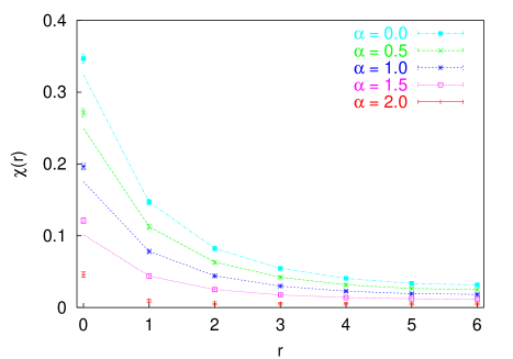
Figure 4: Data for $\chi^{\alpha}(r)$ for $\alpha=0$, …, 2 in steps of $0.5$ (from top to bottom). For $\alpha\neq 2$ we display the best fits using $a+bG_{c}(r)$. (The data are for $T=0.5$.)

Put all together, these analyses strongly favor a power law decrease with $r$ when $\alpha\neq 2$ with a power that is consistent with being $\alpha$-independent. To leading orders one then has

$$\chi^{\alpha\neq 2}(r)\approx\frac{2-\alpha}{3}\sigma_{|q|}^{2}+\frac{B}{r^{\lambda}}$$ (37)

where $\sigma_{|q|}^{2}$ is the variance of $|q|$. In our data, $\lambda=d-c$ is compatible with being an $\alpha$-independent constant whose value is close to $0.5$. This value may be compared to the value $\theta=0.20$ expected within the scaling/droplet picture, and to the exponent $(3/4)(d-2+\eta)$ predicted using scaling arguments within the replica field theory calculation (equal to $0.49$ or $0.585$, according to the numerical estimate of $\eta$ used in the formula - see Sec. III.3.2). In contrast, when $\alpha=2$, our data favor instead the fit to an exponential decrease with $r$, and thus supports the extrapolation of the $d>6$ theoretical analysis of the near-infrared behaviour down to $d=3$.

VI Discussion

We have investigated the properties of certain correlation functions in spin glasses involving two spins. As a first result, we have found that the large distance behavior of the two connected correlation functions $G_{1}$ and $G_{2}$ (see Eq. (4)) satisfies

$$\alpha G_{1}(\infty)+(1-\alpha)G_{2}(\infty)=\frac{2-\alpha}{3}~{}~{}[\overline{\langle q^{2}\rangle}-\overline{\langle q\rangle}^{2}]$$ (38)

and thus $G_{1}(\infty)=\sigma_{|q|}^{2}/3$ and $G_{2}(\infty)=2\sigma_{|q|}^{2}/3$ where $\sigma_{|q|}^{2}$ is the variance of the absolute value of the overlap, $|q|$. (In all our computations, we assumed the presence of an infinitesimal field: the net effect of that field is to decompose the configuration space, rendering overlaps positive.)

A second series of results concerns the way the correlation functions $G_{1}$ and $G_{2}$ tend toward their limits. We found numerically a decrease close to $1/r^{1/2}$ which is a bit different from the droplet/scaling prediction of $1/r^{\theta}$ since $\theta\approx 0.2$. This power law decay disappears when considering precisely $\alpha=2$, i.e., $2G_{1}(r)-G_{2}(r)$: in that case one has both a limiting value compatible with zero and a very fast decay, suggestive of an exponential law.

All of our analytical predictions are based on replica field theory calculations using an effective Lagrangian; this approach should be reliable in dimensions $d>6$. Nevertheless, the main predictions, namely the limiting values of $G_{1}$ and $G_{2}$ and their approach to their limits, all are corroborated in $d=3$ by our numerical study. Also the prediction of a massive-like regime for $2G_{1}-G_{2}$ seems to be nicely consistent with the numerical findings that show for this correlation a very fast decay.

It is of interest to note that Fisher and Huse FisherHuse86 ; FisherHuse88 and Bray and Moore BrayMoore86 had also suggested that there could be a peculiar behaviour for a longitudinal-like linear combination of $G_{1}$ and $G_{2}$, due to the cancellation of the leading term. More precisely, the claim there was that the power law behaviour would be changed from $\theta\approx 0.2$ to a larger value (determined by the expansion of the zero temperature distribution of the internal fields around $h=0$ - see Sec. 4.1 of BrayMoore86 ). We do not find a decrease compatible with $1/r^{\theta}$ for $G_{1}$ and $G_{2}$ separately, while we find a decay compatible with an exponential law for $2G_{1}-G_{2}$, at least in the near infrared; thus qualitatively, the correspondence with the droplet is not good.

Coming back to our results for the large distance limiting values of $G_{1}$ and $G_{2}$, we can derive a simple “sum rule” as follows. Each term in $\chi^{\alpha}(r)$ can be computed when $|i-j|\to\infty$ via replica moments just as we did in Eq. (6):

$$\lim_{r\to\infty}\overline{\langle S_{i}S_{j}\rangle\langle S_{i}\rangle\langle S_{j}\rangle}=\frac{1}{2}[\overline{\langle q^{2}\rangle}+\overline{\langle q\rangle^{2}}]=\overline{\langle q_{12}q_{13}\rangle}\ ,$$ (39)

and

$$\lim_{r\to\infty}\overline{\langle S_{i}\rangle^{2}\langle S_{j}\rangle^{2}}=\frac{1}{3}[2\overline{\langle q^{2}\rangle}+\overline{\langle q\rangle^{2}}]=\overline{\langle q_{12}q_{34}\rangle}\ ,$$ (40)

where, in the last equalities, the averages $\langle\cdots\rangle$ are performed with respect to a replicated equilibrium measure. We then obtain the following sum rule when using Eq. 38 at $\alpha=2$:

$$\overline{\langle q_{12}^{2}\rangle}-4\overline{\langle q_{12}q_{13}\rangle}+3\overline{\langle q_{12}q_{34}\rangle}=0\ .$$ (41)

It is also possible to derive this relation using arguments based on stochastic stability Guerra96 .

As a final comment, note that within the scaling or droplet pictures, when the distance between $i$ and $j$ diverges one has

$$\lim_{|i-j|\to\infty}\frac{\overline{\langle S_{i}\rangle^{2}\langle S_{j}\rangle^{2}}}{\overline{\langle S_{i}\rangle^{2}}~{}~{}\overline{\langle S_{j}\rangle^{2}}}=1\ .$$ (42)

This does not hold in the presence of replica symmetry breaking, and instead we have a relation following from Eq. (40).

Several questions remain open. One would like to determine analytically the power law decrease of $G_{1}$ and $G_{2}$ which here was compatible with $1/r^{1/2}$; is that the exact value, and what is it in higher dimensions? Another issue is related to the presence of the massive-like behaviour for the $\alpha=2$ correlation function in the near-infrared. It would be important to get some analytical estimates of the range where this behaviour does hold also in $d=3$. Finally, one may wonder whether there is any deep reason for the cancellation of the leading parts of $G_{1}$ and $G_{2}$ for $\alpha=2$. One may imagine that it is somehow related to sum rules. Then one may conjecture that to each sum rule for overlaps (obtained for instance using stochastic stability), there is an associated correlation function which decays to zero anomalously fast. This conjecture should be testable for several sum rules using Monte Carlo methods.

Appendix A Replica Fourier Transform

The Replica Fourier transform is a powerful technique which greatly simplifies the diagonalization and inversion of the fluctuation matrix $G$ (see Eq. (10))). The idea is the following. Convolutions in configuration space become products in Fourier space when appropriately defining a Fourier transform in replica space; thus sums over replica co-distances may be transformed into associated products. Similarly, matrices can be inverted in the replica Fourier space and then transformed back to get the desired expression.

Let us assume that replica objects (matrices, tensors etc.) only depend on replica co-distances, and belong to the hierarchical structure described in Sec. III. The Replica Fourier Transform (RFT) DominicisCarlucci97 is a discretized and generalized version of the algebra introduced in MezardParisi91 . For objects like $q_{ab}$ which depend on a single replica co-distance $a\cap b=t$ the RFT ${q}_{\hat{k}}$ is defined as

$${q}_{\hat{k}}=\sum_{t=k}^{R+1}p_{t}(q_{t}-q_{t-1})\ ,$$ (43)

where the $p_{t}$ are the sizes of the Parisi blocks, and objects with indices out of the range of definition are taken as equal to zero.

The inverse transform is given by:

$$q_{t}=\sum_{k=0}^{t}\frac{1}{p_{k}}({q}_{\hat{k}}-{q}_{\widehat{k+1}})\ .$$ (44)

With these definitions, the convolution $\sum_{c}A_{ac}B_{cb}=C_{ab}$ becomes in RFT ${A}_{\hat{k}}{B}_{\hat{k}}={C}_{\hat{k}}$. However, in our case the problem is slightly more complicated. Starting from the known expression of the fluctuation matrix $M$ of Eq. (18), we want to compute the propagator $G=M^{-1}$. Since both $M$ and $G$ are tensors bearing four indices, the unitarity equation $\sum_{cd}M^{ab;cd}G^{cd;ef}=\delta_{ab;ef}$ involves a double convolution in replica space. If the fluctuation matrix and the propagator are expressed in terms of replica co-distances, as described in Eqs. (19) and (20), one needs to Replica Fourier transform with respect to lower indices (i.e., the indices referring to the cross-overlaps between pairs of replicas).

In the Replicon sector, the double transform reads:

$$M_{\hat{k},\hat{l}} = \sum_{u=k}^{R+1}p_{u}\sum_{v=l}^{R+1}p_{v}$$

$$\left(M^{r,r}_{u,v}-M_{u-1,v}^{r,r}-M^{r,r}_{u,v-1}+M^{r,r}_{u-1,v-1}\right)\ ,$$

with, by definition, $k,l\geq r+1$. The inverse transformation can be obtained by applying twice the inverse RFT defined in Eq. (44). From the Lagrangian, Eq. (III.1), we can easily recover the explicit expression of the fluctuation matrix. One has (with the notation of Sec. III.2):

$$M_{R+1,R+1}^{r,r} = p^{2}-2(\tau+uq_{r}^{2})\ ,$$

$$M_{u,R+1}^{r,r} = -wq_{u}\ ,$$

$$M_{R+1,v}^{r,r} = -wq_{v}\ .$$ (46)

From this, by noting that the mean-field solution gives in Replica Fourier space $\tau=-wq_{\hat{0}}$, one gets:

$$M^{r,r}_{\hat{k},\hat{l}}=p^{2}+w[(q_{\hat{0}}-q_{\hat{k}})+(q_{\hat{0}}-q_{\hat{l}})]-2uq^{2}_{r}\ .$$ (47)

In the limit of an infinite number of steps of replica symmetry breaking, $q_{r}\to q(r)$, where now $r\in[0,1]$ while $q(r)$ obeys Eq. (17). Correspondingly, the Replica Fourier transform becomes $q_{\hat{k}}=\int_{k}^{x_{1}}dxxdq/dx-2uq(x_{1})$ and

$$M_{\hat{k},\hat{l}}^{r,r}=p^{2}+\frac{w^{2}}{4u}[k^{2}+l^{2}-2r^{2}]\ .$$ (48)

Finally, by simple inversion, we get the replicon propagator of Eq. (23).

The computation of the longitudinal Fourier component of the propagator is less straightforward. In the longitudinal-anomalous sector the fluctuation matrix $M^{r,s}_{t}$ carries only a lower index (cross-overlap), and thus only one Replica Fourier Transform is needed. However, the lower index runs over a hierarchical tree and when $t$ crosses the upper ‘passive’ indices, the multiplicity may change (sums over replica co-distances such as $r,s,t$ are equivalent to the original sums over replica indices only if the correct multiplicity is taken into account). To deal with this, one has to generalize the definition of Replica Fourier transform in the presence of passive indices:

$$M^{r,s}_{\hat{k}}=\sum_{t=k}^{R+1}p_{t}^{(r,s)}[M^{r,s}_{t}-M^{r,s}_{t-1}]\ ,$$ (49)

with, for $r<s$,

$$p_{t}^{(r,s)} = p_{t}\quad\ \ t\leq r\ ,$$ (50)

$$= 2p_{t}\quad r<t\leq s\ ,$$

$$= 4p_{t}\quad r<s<t\ .$$

With such a definition, the unitarity equation in the longitudinal-anomalous sector becomes:

$$G^{r,s}_{\hat{k}}=-g_{\hat{k}}^{r}[M^{r,s}_{\hat{k}}g_{\hat{k}}^{s}+\sum_{t=0}^{R}M^{r,t}_{\hat{k}}\frac{\delta^{(k-1)}}{4}G^{t,s}_{\hat{k}}]\ ,$$ (51)

where

$$g_{\hat{k}}^{r} = G^{r,r}_{\widehat{r+1},\widehat{r+1}}\quad k\leq r+1\ ,$$ (52)

$$= G^{r,r}_{\widehat{r+1},\hat{k}}\ \ \ \quad k>r+1\ ,$$

and

$$\delta_{t}^{k}=p_{t}^{k}-p_{t+1}^{k}\ .$$ (53)

This equation can be solved with the use of Gegenbauer functions whenever $M^{r,s}_{t}$ depends only on $\min({r,s})$ or on $\max({r,s})$ (see DominicisKondor97 for details). The result for $G^{r,s}_{\hat{0}}$ is the one reported in Eq. (20).

Finally we note that, in the replicon geometry ($r\equiv s$), there is a Longitudinal-Anomalous (LA) contribution to the replicon fluctuation matrix and to the propagator. If we write

$$M^{r,r}_{u,v}=_{R}M^{r,r}_{u,v}+_{A}M^{r,r}_{u,v}\ ,$$ (54)

the LA part can be shown to be DominicisCarlucci97

$${}_{A}M^{r,r}_{u,v}=M^{r,r}_{u}+M^{r,r}_{v}-M^{r,r}_{r}\ .$$ (55)

When performing a double RFT as in Eq. (A), the LA contribution disappears since it bears only one lower index and Eq. (A) is thus a purely replicon contribution.

Appendix B The case of the Heisenberg model

Let us consider the case of the isotropic Heisenberg model with $N$ components. The Hamiltonian for this system reads:

$${\cal H}=\int dx\ \left\{\frac{1}{2}\sum_{i=1}^{N}[(\nabla\Phi_{i})^{2}+\mu\Phi_{i}^{2}]+\frac{g}{4!}\left(\sum_{i=1}^{N}\Phi_{i}^{2}\right)^{2}\right\}$$ (56)

In the low temperature region, for $d>2$, this system develops a spontaneous magnetization ${\vec{M}}$. By expanding Eq. (56) around the mean-field solution $M^{2}=6|\mu|/g$, i.e. ${\vec{\Phi}}={\vec{M}}+{\vec{\phi}}$, we get a field theory where fluctuations along the direction of ${\vec{M}}$ (i.e. longitudinal modes) are massive, while fluctuations transverse to it are massless (zero or Goldstone modes). More precisely,

$${\cal H} = {\cal H}_{mf}+\int dx\left\{\frac{1}{2}[(\nabla\phi_{L})^{2}+(\nabla{\vec{\phi}}_{T})^{2}+\frac{g}{3}M^{2}\phi_{L}^{2}]\right.$$ (57)

$$+ \left.\frac{g}{3!}M\phi_{L}(\phi_{L}^{2}+\phi_{T}^{2})+\frac{g}{4!}(\phi_{L}^{2}+\phi_{T}^{2})^{2}\right\}\ ,$$

where $\phi_{L}$ is the longitudinal mode, and ${\vec{\phi}}_{T}$ the $(N-1)$-dimensional transverse mode. The free propagators then read:

$$G^{0}_{L}(p) = \frac{1}{p^{2}+\frac{g}{3}M^{2}}\ ,$$

$$G^{0}_{T}(p) = \frac{1}{p^{2}}\ .$$ (58)

We now show with a simple argument that, when considering loop corrections, the longitudinal mode, which is massive at the bare level, becomes massless. To see that, let us exhibit the series expansion of the longitudinal propagator $G_{L}$ as in Fig. 5.

Figure 5: Series expansion for the longitudinal propagator in the Heisenberg model.

Here the L-lines correspond to $G_{L}^{0}$ and the wavy lines stand for the magnetization $M$. Since we are interested in the $p\to 0$ limit of $G_{L}(p)$, all other lines are transverse lines, $G^{0}_{T}$. The thin vertices are couplings $g$, the heavy vertices correspond to the effective coupling $\Gamma_{T}$ between transverse modes. We get, integrating out the transverse loops,

$$G_{L}(p)\sim G_{L}^{0}(p)+M\frac{g}{3}G_{L}^{0}(p)\frac{1}{I\ p^{4-d}+\Gamma_{T}(p)}M\frac{g}{3}G_{L}^{0}(p)\ ,$$ (59)

where $I$ is a numerical prefactor.

Figure 6: Effective interaction between transverse modes, obtained by integrating out the longitudinal modes.

The effective transverse interaction can be obtained by integrating out the contribution of the longitudinal modes (see Fig. 6), yielding

$$\Gamma_{T}(p)\sim g-\frac{g^{2}}{3}\frac{1}{p^{2}+\frac{g}{3}M^{2}}=\frac{g\quad p^{2}}{p^{2}+\frac{g}{3}M^{2}}\ .$$ (60)

Thus, $\Gamma_{T}(p)$ vanishes in the infrared limit $p\to 0$ and the Goldstone modes are effectively free. Inserting this expression in Eq. (59), we see that the massive bare behavior $1/[p^{2}+(g/3)M^{2}]$ of the longitudinal propagator is changed into a massless one $1/p^{4-d}$.

This simple argument cannot be applied to the Ising spin glass. Indeed there the Goldstone modes are the bottom of a (transverse) band with no gap separating the massless from the massive modes (see DominicisKondor97 ). As a result, zero modes remain coupled in the infrared, i.e., $\Gamma_{T}(p=0)\neq 0$, and they develop an anomaly.

References

- (1) M. Mézard, G. Parisi, and M. A. Virasoro, Spin-Glass Theory and Beyond, Vol. 9 of Lecture Notes in Physics (World Scientific, Singapore, 1987).
- (2) Spin Glasses and Random Fields, edited by A. P. Young (World Scientific, Singapore, 1998).
- (3) A. J. Bray and M. A. Moore, in Heidelberg Colloquium on Glassy Dynamics, Vol. 275 of Lecture Notes in Physics, edited by J. L. van Hemmen and I. Morgenstern (Springer, Berlin, 1986), pp. 121–153.
- (4) D. S. Fisher and D. A. Huse, Phys. Rev. Lett. 56, 1601 (1986).
- (5) G. Parisi, Phys. Lett. 73A, 203 (1979).
- (6) G. Parisi, Phys. Rev. Lett. 43, 1754 (1979).
- (7) G. Parisi, J. Phys. A Lett. 13, L115 (1980).
- (8) G. Parisi, J. Phys. A 13, 1101 (1980).
- (9) E. Marinari, G. Parisi, and J. Ruiz-Lorenzo, Phys. Rev. B 58, 14852 (1998).
- (10) D. S. Fisher and D. A. Huse, Phys. Rev. B 38, 386 (1988).
- (11) D. Sherrington and S. Kirkpatrick, Phys. Rev. Lett. 35, 1792 (1975).
- (12) C. De Dominicis, I. Kondor, and T. Temesvari, in Spin Glasses and Random Fields, edited by A. P. Young (World Scientific, Singapore, 1998).
- (13) S. F. Edwards and P. W. Anderson, J. Phys. F: Met. Phys. 5, 965 (1975).
- (14) C. De Dominicis, D. Carlucci, and T. Temesvari, J. Phys I France 7, 105 (1997).
- (15) D. Carlucci, Ph.D. thesis, Scuola Normale Superiore, Pisa, Italy, 1997.
- (16) E. Brézin and D. J. Wallace, Phys. Rev. B 7, 1967 (1973).
- (17) E. Brézin, D. J. Wallace, and K. G. Wilson, Phys. Rev. B 7, 232 (1973).
- (18) N. Kawashima and A. P. Young, Phys. Rev..B 53, R484 (1996)
- (19) P. O. Mari and I. A. Campbell, Phys. Rev. E 59 , 2653 (1999).
- (20) K. Hukushima and K. Nemoto, J. Phys. Soc. Jpn. 65, 1604 (1996), cond-mat/9512035.
- (21) F. Zuliani, Ph.D. thesis, University of Cagliari, Cagliari, Italy, 1998.
- (22) E. Marinari, in Advances in Computer Simulation, edited by J. Kertész and I. Kondor (Springer-Verlag, Berlin, 1988), p. 50.
- (23) S. Ciliberti and E. Marinari, J. Stat. Phys. 115, 557 (2004).
- (24) E. Marinari, R. Monasson, and J. Ruiz-Lorenzo, J. Phys. A: Math. and Gen. 28, 3975 (1995), cond-mat/9503074.
- (25) R. Friedberg and O. Martin, J. Phys. A: Math. Gen. 20, 5095 (1987).
- (26) F. Guerra, Int. J. Mod. Phys. B 10, 1675 (1996).
- (27) M. Mézard and G. Parisi, J. Phys. I1, 809 (1991).