Two-cycles in spin-systems: multi-state Ising-type ferromagnets

Abstract

Hamiltonians for general multi-state spin-glass systems with Ising symmetry are derived for both sequential and synchronous updating of the spins. The possibly different behaviour caused by the way of updating is studied in detail for the (anti)-ferromagnetic version of the models, which can be solved analytically without any approximation, both thermodynamically via a free-energy calculation and dynamically using the generating functional approach. Phase diagrams are discussed and the appearance of two-cycles in the case of synchronous updating is examined. A comparative study is made for the $Q$-Ising and the Blume-Emery-Griffiths ferromagnets and some interesting physical differences are found. Numerical simulations confirm the results obtained.

1 Introduction

Recently, there has been renewed interest in the possibly different physics arising from the sequential or synchronous execution of the microscopic update rule of the spins in disordered systems. For example, the Little- Hopfield model on a random graph PS03 and random field Ising chains SC00 , both with synchronous updating have been studied. For both systems governed by a pseudo- Hamiltonian of binary Ising spins (i.e., a Hamiltonian dependent on the inverse temperature) first derived by Peretto P84 , it has been shown that the physics is asymptotically identical to that of the sequential version of the models. Furthermore, for a class of attractor neural networks with spatial structure (one dimensional nearest-neighbour interactions and infinite-range interactions) governed again by Peretto’s pseudo-Hamiltonian it has been found SC200 that dynamical transition lines for synchronous updating in parameter space are exact reflections in the origin of those in sequential updating and that the relevant macroscopic observables can be obtained from those of sequential updating via simple transformations.

It is yet unclear to what extent the two types of spin updating lead to such common equilibrium features. For example, it is known that the phase diagram of the sequential and synchronous Hopfield neural network model in the replica-symmetric approximation are different (e.g. the retrieval region is slightly larger in the synchronous case) FK88 whereas the phase diagram of the Sherrington-Kirkpatrick (SK) spin-glass model SK72 remains unaffected by this difference in updating Nreport .

The aim of this work is to get more insight in the possible differences between sequential and synchronous updating by studying more complicated models containing multi-state spins. In particular, we look at the $Q$-Ising and Blume-Emery-Griffiths (BEG) (anti)-ferromagnetic models which can also be related to a neural network model storing only one pattern. We discuss the relevant phase diagrams as well as the dynamics using the generating functional approach. We are not aware of any previous studies comparing these two types of updating for these models. It turns out that for the $Q$-Ising model again the transition lines for synchronous updating in parameter space are exact reflections of those in sequential updating. For the BEG model, however, the two forms of updating lead to different physics in part of the parameter space.

The paper is organized as follows. In section 2, we generalize the results of Peretto by writing down (pseudo) Hamiltonians based on the detailed balance property for multi-state spin models with random interactions for both sequential and synchronous updating. In the zero- temperature limit the corresponding Lyapunov functions are obtained. In section 3, the phase diagrams for the $Q$-Ising (anti)-ferromagnets are studied in detail, emphasizing the differences between both forms of spin updating. Section 4 discusses the statics of the BEG (anti)-ferromagnet and section 5 the dynamics using the generating functional approach. Numerical simulations confirm the results obtained. Finally, in section 6 some concluding remarks are presented.

2 Models and Hamiltonians

2.1 The $Q$-Ising model

Consider a model of $N$ spins which can take values $\sigma_{i},i=1,\ldots,N$ from a discrete set ${\cal S}=\{-1=s_{1}<s_{2}<\ldots<s_{Q}=+1\}$. Given the configuration ${\mbox{\boldmath$\sigma$}}(t)\equiv\{\sigma_{i}(t)\},i=1,\ldots,N$, the local field in spin $i$ equals

$$h_{i}({\mbox{\boldmath$\sigma$}}(t))=\sum_{j=1}^{N}J_{ij}\sigma_{j}(t)$$ (1)

with $J_{ij}$ the interaction between spin $i$ and spin $j$. In general, the $J_{ij}$ are quenched random variables chosen according to a certain distribution, e.g. a Gaussian in the case of the SK model or a Hebbian learning rule in the case of neural networks.

A spin is updated through the spin-flip dynamics defined by the transition probability

$$\Pr\{\sigma_{i}(t+1)=s_{k}\in{\cal S}|\mbox{\boldmath$\sigma$}(t)\}=\frac{\exp[-\beta\epsilon_{i}(s_{k}|\mbox{\boldmath$\sigma$}(t))]}{\sum_{s\in{\cal S}}\exp[-\beta\epsilon_{i}(s|\mbox{\boldmath$\sigma$}(t))]}\,.$$ (2)

Here the energy potential $\epsilon_{i}[s|{\mbox{\boldmath$\sigma$}}]$ is defined by R90

$$\epsilon_{i}[s|{\mbox{\boldmath$\sigma$}}]=-\left[\frac{1}{2}h_{i}({\mbox{\boldmath$\sigma$}})s-bs^{2}\right]\,,$$ (3)

where $b$ is the gain parameter of the system. The zero temperature limit $T=\beta^{-1}\rightarrow 0$ of this dynamics is given by the updating rule

$$\sigma_{i}(t)\rightarrow\sigma_{i}(t+1)=s_{k}:\min_{s\in{\cal S}}\epsilon_{i}[s|{\mbox{\boldmath$\sigma$}}(t)]=\epsilon_{i}[s_{k}|{\mbox{\boldmath$\sigma$}}(t)]\,.$$ (4)

This updating rule (4) is equivalent to using a gain function $\mbox{g}_{b}(\cdot)$,

$$\sigma_{i}(t+1)=\mbox{g}_{b}(h_{i}(\mbox{\boldmath$\sigma$}(t))$$

$$\mbox{g}_{b}(x)\equiv\sum_{k=1}^{Q}s_{k}\left[\theta\left[b(s_{k+1}+s_{k})-x\right]-\theta\left[b(s_{k}+s_{k-1})-x\right]\right]$$

with $s_{0}\equiv-\infty$ and $s_{Q+1}\equiv+\infty$. The parameter $b$ suppresses or enhances the states of the spins that lie around the zero state.

In the case of sequential updating it is well-known from detailed balance arguments that for symmetric couplings, i.e., $J_{ij}=J_{ji}$, and in the absence of self-interactions, i.e., $J_{ii}=0$, the equilibrium distribution for the $Q$-Ising system has the Boltzmann form with Hamiltonian (see, e.g., GS77 )

$$H_{S}(\mbox{\boldmath$\sigma$})=-\frac{1}{2}\sum_{i,j\neq i}^{N}J_{ij}\sigma_{i}\sigma_{j}+b\sum_{i=1}^{N}\sigma_{i}^{2}\,,$$ (6)

valid for any temperature and with Lyapunov behaviour for $T=0$. We remark that the second term is not a self coupling term. As in any spin model with sequential updating, the stationary solutions can only be fixed points.

For synchronous updating a discussion does not seem to have appeared in the literature. In that case, the arguments of Peretto P84 can be generalized rather straightforwardly to obtain that again the equilibrium probability distribution can be written in the Boltzmann form with a Hamiltonian dependent on the inverse temperature

$$H_{P}(\mbox{\boldmath$\sigma$})=-\frac{1}{\beta}\sum_{i=1}^{N}\ln{\left[\sum_{s\in\mathcal{S}}\exp{(\beta[h_{i}(\mbox{\boldmath$\sigma$})s-bs^{2}])}\right]}+b\sum_{i=1}^{N}\sigma_{i}^{2}$$ (7)

We remark that self-couplings $J_{ii}$ are allowed to be present. This pseudo-Hamiltonian can be written in a two-spin representation

$$H_{P}(\mbox{\boldmath$\sigma$},\mbox{\boldmath$\tau$}) = -\frac{1}{\beta}\sum_{i,j\neq i}J_{ij}\sigma_{i}\tau_{j}+b\sum_{i}(\sigma_{i}^{2}+\tau_{i}^{2})$$

$$= -\frac{1}{\beta}\sum_{i,j\neq i}J_{ij}\sigma_{i}(t)\sigma_{j}(t+1)$$

$$+ b\sum_{i}[\sigma_{i}^{2}(t)+\sigma_{i}^{2}(t+1)]$$ (9)

In the limit $\beta\rightarrow\infty$ we find after some algebra starting from (7)

$$H_{P}(\mbox{\boldmath$\sigma$};T=0)$$ (10)

$$=-\sum_{i=1}^{N}\sum^{Q}_{j=[\frac{Q+3}{2}]}\left(|h_{i}(\mbox{\boldmath$\sigma$})|s_{j}-bs_{j}^{2}\right)$$

$$\times\theta\left(|h_{i}(\mbox{\boldmath$\sigma$})|-b(s_{j-1}+s_{j})\right)$$

$$\times\theta\left(b(s_{j}+s_{j+1})-|h_{i}(\mbox{\boldmath$\sigma$})|\right)+b\sum_{i=1}^{N}\sigma_{i}^{2}$$

with the standard notation $[\cdot]$ indicating the largest integer. For $Q=2$, we find back the Hopfield Hamiltonian with an irrelevant additive constant. For $Q=3$ we have

$$H_{P}(\mbox{\boldmath$\sigma$};T=0)=-\sum_{i=1}^{N}\left(|h_{i}(\mbox{\boldmath$\sigma$})|-b\right)\theta\left(|h_{i}(\mbox{\boldmath$\sigma$})|-b\right)+b\sum_{i=1}^{N}\sigma_{i}^{2}$$ (11)

The Hamiltonian for general $Q$ is bounded from below by $H_{P}(\mbox{\boldmath$\sigma$};T=0)\geq-\sum_{i,j\neq i}|J_{ij}|-N|b|$ and, furthermore

$$\Delta H_{P}(\mbox{\boldmath$\sigma$};T=0) \equiv H_{P}(\mbox{\boldmath$\sigma$}(t+1);T=0)-H_{P}(\mbox{\boldmath$\sigma$}(t);T=0)$$

$$=-\sum_{i=1}^{N}\left(\sigma_{i}(t+2)-\sigma_{i}(t)\right)$$

$$\times\left(h_{i}(\mbox{\boldmath$\sigma$}(t+1))-b(\sigma_{i}(t+2)+\sigma_{i}(t))\right)\leq 0$$

indicating that the equilibrium behaviour can be fixed-points and/or cycles of period $2$, i.e., $\sigma_{i}(t)=\sigma_{i}(t+2)$, $\forall i$.

2.2 The BEG model

The second model we consider is the BEG model introduced in BEG71 in the context of the $\lambda$-transition and phase separation in the mixtures of $He^{3}-He^{4}$ in a crystal field, and recently discussed as a spin-glass (see ACN00 ; CL04 and references therein) and as a neural network model maximising the mutual information content for ternary neurons DK00 ; toni ; B04 . This model can be described as follows.

Consider $N$ spins which can take values $\sigma_{i},i=1,\ldots,N$ from a discrete set ${\cal S}=\{-1,0,+1\}$. Given the configuration ${\mbox{\boldmath$\sigma$}}(t)\equiv\{\sigma_{i}(t)\},i=1,\ldots,N$ at time $t$, the spins are updated according to the spin-flip dynamics defined by the transition probability (2) where the energy potential $\epsilon_{i}[s|{\mbox{\boldmath$\sigma$}}(t)]$ is now defined by

$$\epsilon_{i}[s|{\mbox{\boldmath$\sigma$}}(t)]=-(h_{1,i}(\mbox{\boldmath$\sigma$}(t))s+h_{2,i}(\mbox{\boldmath$\sigma$}(t))s^{2})\,.$$ (13)

The local field $h_{1,i}(\mbox{\boldmath$\sigma$})$ is the usual one as appearing, e.g., in (3), while the biquadratic $h_{2,i}(\mbox{\boldmath$\sigma$})$ local field is given by

$$h_{2,i}(\mbox{\boldmath$\sigma$}(t))=\sum_{j=1}^{N}K_{ij}\sigma_{j}^{2}(t)\,.$$ (14)

In the limit $\beta\rightarrow\infty$ this dynamics is given by the updating rule

$$\sigma_{i}(t+1)=\mbox{sign}(h_{1,i}(\mbox{\boldmath$\sigma$}(t)))\theta\left(|h_{1,i}(\mbox{\boldmath$\sigma$}(t))|+h_{2,i}(\mbox{\boldmath$\sigma$}(t))\right)$$ (15)

In the case of sequential updating of the spins the Hamiltonian is known in the literature mentioned above and given by

$$H^{BEG}_{S}(\mbox{\boldmath$\sigma$})=-\frac{1}{2}\sum_{i,j\neq i}^{N}\left(J_{ij}\sigma_{i}\sigma_{j}+K_{ij}\sigma_{i}^{2}\sigma_{j}^{2}\right)$$ (16)

with $J_{ii}=0$ and $J_{ij}=J_{ji}$, for $\forall i,j$.

For synchronous updating detailed balance and symmetry in the couplings lead to the pseudo-Hamiltonian

$$H_{P}^{BEG}(\mbox{\boldmath$\sigma$})=-\frac{1}{\beta}\sum_{i=1}^{N}\ln{\left\{2e^{\beta h_{2,i}(\mbox{\boldmath$\sigma$})}\cosh{(\beta h_{1,i}(\mbox{\boldmath$\sigma$}))}+1\right\}}$$ (17)

with as two-spin representation

$$H_{P}^{BEG}(\mbox{\boldmath$\sigma$},\mbox{\boldmath$\tau$})$$

$$=-\sum_{i,j\neq i}\left(J_{ij}\sigma_{i}\tau_{j}+K_{ij}\sigma_{i}^{2}\tau_{j}^{2}\right)$$ (18)

$$\equiv-\sum_{i,j\neq i}\left(J_{ij}\sigma_{i}(t)\sigma_{j}(t+1)+K_{ij}\sigma_{i}^{2}(t)\sigma_{j}^{2}(t+1)\right)$$ (19)

Determining the dominant contributions in the limit $\beta\rightarrow\infty$ we find

$$H^{BEG}_{P}(\mbox{\boldmath$\sigma$},\mbox{\boldmath$\tau$};T=0)=-\sum_{i=1}^{N}\left(|h_{1,i}(\mbox{\boldmath$\sigma$})|+h_{2,i}(\mbox{\boldmath$\sigma$})\right)\\ \times\theta\left(|h_{1,i}(\mbox{\boldmath$\sigma$})|+h_{2,i}(\mbox{\boldmath$\sigma$})\right)\,.$$ (20)

This form is clearly bounded from below and it can also be shown that the equilibrium behaviour is given by fixed-point attractors and/or cycles of period $2$.

Both the $Q$-Ising and BEG spin-glass models and neural networks have been discussed in the literature starting from the Hamiltonian appropriate for sequential updating of the spins, as discussed in the introduction. Concerning synchronous updating, especially concerning the appearance and properties of two-cycles, very little seems to be written down, even for the ferromagnetic versions of these models. Since interesting different physics is involved we want to fill this gap in the following sections.

3 $Q$-Ising ferromagnet: sequential versus synchronous updating

3.1 Stationary behaviour

We consider the $Q$-Ising (pseudo)-Hamiltonians for sequential and synchronous updating derived before for simplified interactions of the form

$$J_{ij}=\frac{J}{N}$$ (21)

where $J$ can be positive or negative. The parameters describing the properties of this system are the magnetization $m$ and the spin activity $a$ given by

$$m(\mbox{\boldmath$\sigma$})=\frac{1}{N}\sum_{i}\sigma_{i}\,,\quad a(\mbox{\boldmath$\sigma$})=\frac{1}{N}\sum_{i}\sigma_{i}^{2}$$ (22)

and in both cases the equilibrium behaviour can be studied by looking at the free energy per site,

$$f=\frac{-1}{\beta N}\ln{Z}\,,\quad Z=\sum_{\sigma}\exp{(-\beta H(\mbox{\boldmath$\sigma$}))}.$$ (23)

For sequential updating starting from the Hamiltonian (6) a standard calculation leads to the following free energy

$$\beta f_{S}=\underset{m}{\mbox{extr}}\left[\frac{\beta J}{2}m^{2}-\ln\sum_{\sigma}\exp({-\beta\tilde{H}(\sigma))}\right]$$ (24)

with the effective Hamiltonian

$$\tilde{H}_{S}(\sigma)=-Jm\sigma+b\sigma^{2}\ .$$ (25)

The saddle-point equation for $m$ in this notation reads

$$m=\frac{\sum_{\sigma}\sigma\exp({-\beta\tilde{H}(\sigma)})}{\sum_{\sigma}\exp({-\beta\tilde{H}(\sigma)})}\equiv\left\langle\sigma\right\rangle$$ (26)

which is an effective thermal average, denoted by $\left\langle\cdot\right\rangle$.

In the case of synchronous updating we start from the pseudo-Hamiltonian written in the two-spin representation (2.1). This Hamiltonian is symmetric with respect to the transformation $\sigma\leftrightarrow\tau$. The following result for the free energy is obtained

$$\beta f_{P}=\underset{m_{\sigma},m_{\tau}}{\mbox{extr}}\left[\beta Jm_{\sigma}m_{\tau}-\ln\sum_{\sigma,\tau}\exp({-\beta\tilde{H}(\sigma,\tau)})\right]$$ (27)

with the effective Hamiltonian

$$\tilde{H}(\sigma,\tau)=-Jm_{\tau}\sigma-Jm_{\sigma}\tau+b\sigma^{2}+b\tau^{2}\ .$$ (28)

The saddle-point equations for $m_{\sigma}$ and $m_{\tau}$ read

$$m_{\sigma}=\frac{\sum_{\sigma,\tau}\sigma\exp({-\beta\tilde{H}(\sigma,\tau)})}{\sum_{\sigma,\tau}\exp({-\beta\tilde{H}(\sigma,\tau)})}=\left\langle\sigma\right\rangle$$ (29)

$$m_{\tau}=\frac{\sum_{\sigma,\tau}\tau\exp({-\beta\tilde{H}(\sigma,\tau)})}{\sum_{\sigma,\tau}\exp({-\beta\tilde{H}(\sigma,\tau)})}=\left\langle\tau\right\rangle\ ,$$ (30)

where this again defines the average $\left\langle\cdot\right\rangle$.

The effective Hamiltonian factorises over the two effective spins, and so does the partition function. The saddle-point equations for $m_{\sigma}$ and $m_{\tau}$ (29)-(30) can be written as

$$m_{\sigma}=F_{Q}(m_{\tau})\ ,\qquad m_{\tau}=F_{Q}(m_{\sigma})$$ (31)

with the function $F_{Q}$ given by

$$F_{Q}(x)=\frac{\sum_{\sigma}\sigma\exp{\beta(Jx\sigma-b\sigma^{2})}}{\sum_{\sigma}\exp{\beta(Jx\sigma-b\sigma^{2})}}\ .$$ (32)

The equations (31) can be written as

$$m_{\sigma}=F_{Q}(F_{Q}(m_{\sigma}))\,,\quad m_{\tau}=F_{Q}(F_{Q}(m_{\tau}))$$ (33)

and similar equations can be written down for the activity, for instance

$$a_{\sigma} =G_{Q}(F_{Q}(m_{\sigma})),$$

$$G_{Q}(x) =\frac{\sum_{\sigma}\sigma^{2}\exp{\beta(Jx\sigma-b\sigma^{2})}}{\sum_{\sigma}\exp{\beta(Jx\sigma-b\sigma^{2})}}\,.$$ (34)

At this point we remark that the saddle-point equation for the sequential $Q$-Ising model (26) is equivalent to $m=F_{Q}(m)$ and the activity satisfies $a=G_{Q}(m)$.

For $J>0$ the function $F_{Q}(x)$ is monotonically increasing since

$$\frac{\partial F_{Q}(x)}{\partial x} = \beta J\left[\rule{0.0pt}{17.07182pt}\frac{\sum_{\sigma}\sigma^{2}\,\exp{\beta(Jx\sigma-b\sigma^{2})}}{\sum_{\sigma}\exp{\beta(Jx\sigma-b\sigma^{2})}}\right.$$ (35)

$$-\left.\left(\frac{\sum_{\sigma}\sigma\,\exp{\beta(Jx\sigma-b\sigma^{2})}}{\sum_{\sigma}\exp{\beta(Jx\sigma-b\sigma^{2})}}\right)^{2}\right]\geq 0\ .$$

Consequently the right-hand side of

$$(m_{\sigma}-m_{\tau})^{2}=(m_{\sigma}-m_{\tau})(F_{Q}(m_{\tau})-F_{Q}(m_{\sigma}))$$ (36)

is always negative implying that $m_{\sigma}=m_{\tau}$ and

$$f_{P}=2f_{S}\ .$$

In other words, the equilibrium states for both types of updating in the ferromagnetic $Q$-Ising model are the same. For $J<0$, and also for the BEG-model, this is not valid as we will see in the following sections.

3.2 An illustrative example: $Q=3$

The results for $Q=2$ are standard textbook knowledge (see, e.g, C01s ). For $Q=3$, the equations for $F_{Q}$ and $G_{Q}$ can be worked out explicitly

$$F_{Q=3}(x)=\frac{2\sinh{(\beta Jx)}}{\exp{(\beta b)}+2\cosh{(\beta Jx)}}$$ (37)

$$G_{Q=3}(x)=F_{Q=3}(x)\coth{(\beta Jx)}\,.$$ (38)

The phase diagram for sequential updating is shown in fig. 1.

Figure 1: Phase diagram for the sequential $Q=3$ Ising ferromagnet. The thick dashed (solid) line indicates the thermodynamic second (first) order transition between the ferromagnet and paramagnetic phase. The thin lines border the coexistence region.

It is trivial to check that a negative $J$ implies that $m=F_{Q=3}(m)$ only leads to a stable paramagnetic solution $m=0$. For positive $J$ a transition occurs between the paramagnetic and the ferromagnetic phase. It is second order and given by the dashed line

$$a=\frac{1}{\beta J},\qquad\beta b=\ln{(2(\beta J-1))}$$ (39)

for $\beta J<3.01$ and $\beta b<1.39$. It is first order above this tricritical point and given there by the thick solid line, which is the thermodynamic transition line found by comparing free energies. Starting in the ferromagnetic phase for $\beta J>3.01$ and letting $\beta b$ become bigger we arrive at the first solid line where also the paramagnetic solution starts to be stable and, hence, the coexistence region $II$ begins. This line is given by (39). At the thick full line, this paramagnetic solution becomes the global minimum of the free energy and at the second thin solid line given by

$$m(coth(\beta J)-m)=\frac{1}{\beta J}$$ (40)

the ferromagnetic solution stops existing. It is interesting to remark that inside the $m=0$ phase, for any $\beta J$ and $\beta b\geq 2.89$ only 10% or less of the spins remain in states $\pm$1 Furthermore, the phase diagram in the region of negative $b$ is rather trivial since negative $b$ tend to suppress all the zero states in the system.

For synchronous updating the equations (33)-(34) are invariant under a change of sign of $J$, such that the corresponding $\beta J-\beta b$ phase diagram will be symmetric with respect to the axis $J=0$. Furthermore, as shown before, the sequential and synchronous Q-Ising models have exactly the same stationary states for any $J>0$. Therefore, the phase diagram is straightforwardly given in figure 2.

Figure 2: Phase diagram of the synchronous $Q=3$ Ising ferromagnet. The lines are as in fig. 1

However, some caution is required here. From a study of the dynamics, similar to the one presented for the BEG-model in the next section, one becomes aware of the difference between the regions $J>0$ and $J<0$. For positive $J$, all stationary solutions are fixed-points, while for negative $J$ the $m=0$ solution (stable in $I$ and $II$) is of the same nature as for $J>0$. The $m\neq 0$ solution (stable in $II$ and $III$) is a two-cycle, and the system jumps from $m$ to $-m$ with the activity $a$ constant.

4 BEG ferromagnet: statics for sequential and synchronous updating

We recall the (pseudo)-Hamiltonian for sequential and synchronous updating (16) respectively (17) and choose ferromagnetic couplings

$$J_{ij}=\frac{J}{N},\quad K_{ij}=\frac{K}{N}\,.$$ (41)

The order parameters describing the properties of the system are defined as in (22).

For sequential updating a standard calculation leads to the free energy

$${\beta}f_{S}=\underset{m,a}{\mbox{extr}}\left\{\frac{1}{2}\beta Jm^{2}+\frac{1}{2}\beta Ka^{2}\right.$$

$$+\left.\ln{\left[\rule{0.0pt}{12.80365pt}2\exp{(\beta Ka)}\cosh{(\beta Jm)}+1\right]}\right\}$$ (42)

and the following fixed-point equation must be satisfied

$$m=\frac{2\sinh{(\beta Jm)}}{\exp{(-\beta Ka)}+2\cosh{(\beta Jm)}}$$ (44)

$$a=\frac{2\cosh{(\beta Jm)}}{\exp{(-\beta Ka)}+2\cosh{(\beta Jm)}}\,.$$

For synchronous updating the free energy becomes

$${\beta}f_{P}=\underset{m_{\sigma},m_{\tau},a_{\sigma},a_{\tau}}{\mbox{extr}}\left\{\beta Jm_{\sigma}m_{\tau}+\beta Ka_{\sigma}a_{\tau}\right.$$

$$\left.+\ln\left[\left(2\exp{(\beta Ka_{\sigma})}\cosh{(\beta Jm_{\sigma})}+1\right)\right.\right.$$

$$\quad\times\left.\left.\left(2\exp{(\beta Ka_{\tau})}\cosh{(\beta Jm_{\tau})}+1\right)\right]\right\}$$ (45)

with $m_{\sigma},m_{\tau},a_{\sigma},a_{\tau}$ satisfying the saddle-point equations

$$m_{\sigma}=F_{BEG}(m_{\tau},a_{\tau})\ ,\quad m_{\tau}=F_{BEG}(m_{\sigma},a_{\sigma})$$ (46)

$$a_{\sigma}=G_{BEG}(m_{\tau},a_{\tau})\ ,\quad a_{\tau}=G_{BEG}(m_{\sigma},a_{\sigma})$$ (47)

and the functions $F_{BEG},G_{BEG}$ given by

$$F_{BEG}(x,y)=\frac{2\sinh{(\beta Jx)}}{\exp{(-\beta Ky)}+2\cosh{(\beta Jx)}}$$ (48)

$$G_{BEG}(x,y)=F_{BEG}(x)\coth{(\beta Jx)}\,.$$ (49)

It is clear that the results for sequential updating can then be written as

$$m=F_{B}(m,a)\ ,\quad a=G_{B}(m,a)$$ (50)

and the results for synchronous updating satisfy

$$m_{\sigma}=F_{B}(F_{B}(m_{\sigma},a_{\sigma}),G_{B}(m_{\sigma},a_{\sigma}))$$ (51)

$$a_{\sigma}=G_{B}(F_{B}(m_{\sigma},a_{\sigma}),G_{B}(m_{\sigma},a_{\sigma}))$$ (52)

where, for convenience, we have simplified the subscript.

These relations form again the basis for studying the differences and similarities between sequential and synchronous updating in the BEG model. Let us first look at the phase diagram for sequential updating shown in figure 3.

Figure 3: Phase diagram for the sequential BEG ferromagnet. The lines are as in fig. 1

For $J<0$ the only stable solution is given by $m=0$ and the single value $a=G_{B}(0,a)={2}{[2+\exp{(-\beta Ka)}]^{-1}}$. For $J>0$ we see from (44) that, when $m\neq 0$ and $K\neq 0$, $a=m\coth{(\beta Jm)}$.

The transition between the paramagnetic and ferromagnetic phase is given by the dashed line

$$a=\frac{1}{\beta J},\qquad\beta K=-\beta J\ln{(2(\beta J-1))}$$ (53)

in analogy with the transition line (39) for the $Q=3$ Ising ferromagnet. It is second order for all coupling parameters, in contrast with the one for the $Q=3$ Ising model. We remark that inside the paramagnetic phase, only 10% of the spins (or less) remain in the states $\pm 1$ below $\beta K\simeq-28.904$.

For synchronous updating the phase diagram is more involved as can be seen in figure 4. First we note that the set of equations (52) is invariant under the change of sign of $J$, such that the phase diagram is symmetric with respect to the $J=0$ axis.

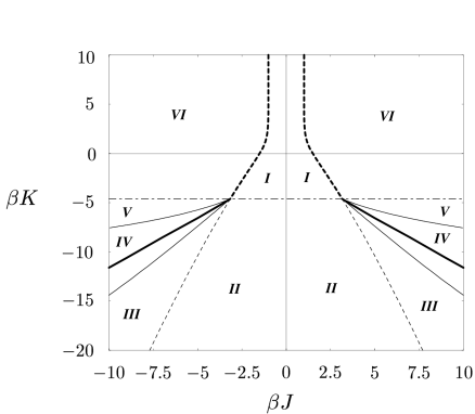
Figure 4: Phase diagram for the synchronous BEG ferromagnet. The dashed-dotted line indicates the bifurcation of solutions in $a$. The rest of the lines is as in fig. 1

In the case $m=0$ one finds from eq. (52) that the equation for $a$ is given by $a=G_{B}(G_{B}(0,a))$. For certain values of $\beta K$, this equation has three solutions bifurcating from the sequential one $a=G_{BEG}(0,a)$ at the following point

$$\beta K=\frac{-1}{a(1-a)},\qquad 1=(1-a)\ln{\left(\frac{2(1-a)}{a}\right)}$$ (54)

giving the result $a^{*}\simeq 0.316$ and $\beta K^{*}\simeq-4.623$. This bifurcation line is indicated in fig. 4 as the dashed-dotted line. It separates the regions I-II and V-VI in the phase diagram. For $\beta K<\beta K^{*}$, the two new solutions appearing at that point become automatically the stable ones in the phases where $m=0$ is stable ($II$, $III$, and $IV$), while the sequential solution becomes unstable. Figure 5 illustrates this behaviour. In region $I$, where only the solution $m=0$ is stable, the unique and stable solution for $a$ is $a=G_{B}(0,a)$. In addition, for $\beta K<\beta K^{*}$ the transition line (53) becomes simply the border where the ferromagnetic solution starts to exist, but is not yet stable, since in region $III$ the ferromagnetic solution is only a minimum of the free energy in the $m$ direction. At this point we remark that in figure 5 still other spurious unstable solutions can be seen, i.e., the loops in the top figure.

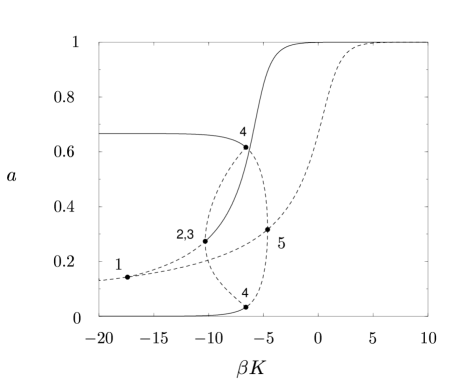
Figure 5: Stationary limit of $m$ and $a$ as a function of $\beta K$ given $\beta J=7$. The same labels correspond to the same points. Solid lines denote stable solutions, while dashed lines indicate unstable ones.

Simulations and the dynamics of the BEG-model discussed in the next section show that in the paramagnetic phase $II$, for $\beta K<\beta K^{*}$, the system oscillates between the two stable solutions for $a$ and, therefore, the equilibrium configuration is a cycle of period 2 where both configurations involved have different $a$ values which become equal to $0$ and $2/3$ when $\beta K\rightarrow-\infty$.

We find that below $\beta K^{*}$ the transition from the paramagnet to the ferromagnet phase becomes first order. Comparing numerically the free energies we find the first order thermodynamic transition indicated by the thick solid lines in fig. 4. The tricritical point is given by $\beta J\simeq\pm 3.160$, $\beta K\simeq-4.623$. As a consequence, as in the $Q=3$ Ising model and in contrast with the sequential BEG model, there is a coexistence region bordered by the thin solid lines. Again, these lines can be obtained analytically. Starting in the stable paramagnetic phase $m=0$ for, to fix ideas, $\beta J=7$ and increasing the value of $\beta K$ we find the following. We first meet the thin dashed line where the ferromagnetic solution $m>0$ appears but is still unstable. This line coincides with the transition line in the sequential BEG model (recall fig. 3) because the sequential solution is also a solution here. In region $III$ this ferromagnetic solution stays unstable until we meet the solid line between regions $III$ and $IV$, being the lower border of the coexistence region. This line is given by the point where the ferromagnetic free energy becomes a (local) minimum in the $a$ direction, i.e.,

$$(2\beta K-a)\frac{\partial G_{B}(m,a)}{\partial a}-(\beta J)^{2}(a^{2}-m^{2})\left(\frac{\partial F_{B}(m,a)}{\partial a}\right)^{2}$$

$$-(1-a)\left[(\beta K)^{2}a(1+\left(\frac{\partial G_{B}(m,a)}{\partial a}\right)^{2}\right.$$

$$\left.+\beta KaG_{B}(m,a)\frac{\partial G_{B}(m,a)}{\partial a}-\beta JmG_{B}(m,a)\frac{\partial F_{B}(m,a)}{\partial a}\right.$$

$$\left.+2\beta J\beta Km\frac{\partial F_{B}(m,a)}{\partial a}\frac{\partial G_{B}(m,a)}{\partial a}\right]=0$$ (55)

where $F_{B}(m,a)$ and $G_{B}(m,a)$ are defined in (48) and (49).

Next, we meet the thermodynamic line discussed before where the ferromagnetic solution becomes a global minimum of the free energy. Increasing $\beta K$ further we arrive at the border of region $IV$ and $V$ where the paramagnetic solution becomes unstable. It is given by

$$\frac{2(\beta J)^{2}a}{\exp({-\beta Ka})+2}=1\,.$$ (56)

This equation has two solutions. The first solution $a=G_{B}(0,a)$ gives the separation line between regions $I$ and $VI$, which corresponds to the transition line in sequential updating (fig. 3). The second solution $a=G_{B}(G_{B}(0,a))\neq G_{B}(0,a)$ gives the upper border of the coexistence region $IV$. The last line we meet is the separation between regions $V$ and $VI$, as found in eq. (54). In regions $V$ and $VI$, only the ferromagnetic solution is stable.

These results allow us to say that sequential and synchronous updating lead to completely the same physics ($f_{P}=2f_{S}$) in the region $\beta J>0$, $\beta K>-4.623$. Hence, as we will further explain in the next section on dynamics there are no cycles for positive couplings, but we do find them for positive $\beta J$ and negative $\beta K$. They turn out to be stable in the regions $II$, $III$ and $IV$.

5 BEG ferromagnet: dynamics for sequential and synchronous updating

The aim of this section is to study the dynamics of the BEG model in order to further examine the difference between sequential and synchronous updating and to further understand the appearance and behaviour of two-cycles. In order to do so we use the generating function (path integral) technique introduced in MSR73 to the field of statistical mechanics and, by now, part of many textbooks. In particular, we follow C01d . Since we have no disorder in our problem, the method can be used in its simplest form.

The probability of a certain microscopic path of spin configurations from time $0$ up to time $t$ is denoted by $\mbox{P}[\mbox{\boldmath$\sigma$}(0),...,\mbox{\boldmath$\sigma$}(t)]$. For the BEG model defined in section 2 it is given by

$$\mbox{P}[\mbox{\boldmath$\sigma$}(0),...,\mbox{\boldmath$\sigma$}(t)]\equiv\mbox{P}_{0}(\mbox{\boldmath$\sigma$}(0))\prod_{s=0}^{t-1}W[\mbox{\boldmath$\sigma$}(s+1);\mbox{\boldmath$\sigma$}(s)]$$ (57)

with $W[\mbox{\boldmath$\sigma$};\mbox{\boldmath$\sigma$}^{\prime}]$ the transition matrix of the Markovian process defined by the spin-flip dynamics given by eqs. (2) and (13). It depends on the specific way of updating the spins (sequential or synchronous) and will be specified later. We introduce a generating function for the BEG model as a function of the field $\bf\Phi$

$$Z[{\bf\Phi}]=\left\langle\exp\left[-i\sum_{s=0}^{t}\sum_{i=1}^{N}\sum_{k=1}^{2}\phi_{k,i}(s)\sigma_{i}^{k}(s)\right]\right\rangle_{path}$$ (58)

where the average $\langle\cdot\rangle_{path}$ is an average over $\mbox{P}[\mbox{\boldmath$\sigma$}(0),...,\mbox{\boldmath$\sigma$}(t)]$. The order parameters of the system are generated by this function $Z[{\bf\Phi}]$ through

$$\langle\sigma_{i}^{k}(s)\rangle_{path}=i\lim_{{\bf\Phi}\rightarrow 0}\left(\frac{\partial Z[{\bf\Phi}]}{\partial\phi_{k,i}(s)}\right)\,.$$ (59)

At this point we remark that, for our purposes, we only look at these one-time quantities. Again, to unify notation we use the “magnetizations” $m_{k}(s)$, $k=1,2$ to denote the magnetization $m(\mbox{\boldmath$\sigma$}(s))$, respectively the spin activity $a(\mbox{\boldmath$\sigma$}(s))$.

Introducing these magnetizations into the generating function (58) by using appropriate $\delta$ functions and grouping the terms in those depending on the site index and those which do not, we obtain

$$Z[{\bf\Phi}]\propto\int\prod_{k}\left[d{\bf m}_{k}d\hat{{\bf m}}_{k}\right]\exp{N\Psi}$$ (60)

with $d{\bf m}_{k}=dm_{k}(0)...dm_{k}(t)$ and similarly for $d\hat{{\bf m}}_{k}$. The quantity $\Psi$ reads

$$\Psi=i\sum_{k,s}\hat{m}_{k}(s)m_{k}(s)$$

$$+\frac{1}{N}\sum_{i}\ln{\left\langle\exp\left[-i\sum_{k,s}\sigma_{i}^{k}(s)(\hat{m}_{k}(s)+\phi_{k,i}(s))\right]\right\rangle_{path}}$$ (61)

This generating function (60) allows for the application of the saddle-point method. In order to continue we need to specify the type of updating.

5.1 Synchronous updating

In this case all spins are updated at the same time such that the transition probabilities $W_{p}[\mbox{\boldmath$\sigma$}(s+1);\mbox{\boldmath$\sigma$}(s)]$ are just the product of the transition probabilities of the single spin (recall eqs. (2) and (13)). Noting that the local fields are equal to $h_{k}(s)\equiv J_{k}m_{k}(s)$ (with obvious definitions for $J_{k}$) we obtain

$$\Psi=i\sum_{k,s}\hat{m}_{k}(s)m_{k}(s)+\frac{1}{N}\sum_{i}\ln\left[\sum_{\mbox{\boldmath$\sigma$}(0)}...\sum_{\mbox{\boldmath$\sigma$}(t)}\mbox{P}_{0}(\mbox{\boldmath$\sigma$}(0))\right.$$

$$\left.\exp{[-i\sum_{k,s}\sigma_{i}^{k}(s)(\hat{m}_{k}(s)+\phi_{k,i}(s)+i\beta J_{k}m_{k}(s-1))]}\right.$$

$$\left.\exp{\bigg{[}-\sum_{s}\ln{\left(1+2e^{\beta J_{2}m_{2}(s-1)}\cosh{(\beta J_{1}m_{1}(s-1))}\right)}\bigg{]}}\right]$$

Choosing the initial conditions $\mbox{P}_{0}(\mbox{\boldmath$\sigma$}(0))$ to be iidrv with respect to $i$ and letting $\phi_{k,i}\rightarrow\phi_{k}$, the single-site nature of the last expression becomes apparent. Defining an effective (i.e., single-site) path average denoted by $\langle\cdot\rangle_{*}$ the saddle-point equations then become

$$m_{k}(s)=\langle\sigma^{k}(s)\rangle_{*}\,,\quad\hat{m}_{k}(s)=0\,.$$ (63)

Working out further details and summing over the spins we easily obtain

$$m_{1}(s) =\frac{2e^{\beta J_{2}m_{2}(s-1)}\sinh{(\beta J_{1}m_{1}(s-1))}}{1+e^{\beta J_{2}m_{2}(s-1)}\cosh{(\beta J_{1}m_{1}(s-1))}}$$ (64)

$$m_{2}(s) =m_{1}(s)\coth(\beta J_{1}m_{1}(s-1))\,.$$ (65)

These saddle-point equations allow for two-cycles when $m_{k}(s)=m_{k}(s+2)$, $k=1,2$ and fixed points with $m_{k}(s)=m_{k}(s+1)$. The stationary limit is obtained when we drop the time dependence, writing $m_{k}(s)$ as $m_{\sigma}$ and $m_{k}(s-1)$ as $m_{\tau}$ or the other way around. Some further discussion and numerical results will be presented after studying sequential updating.

5.2 Sequential updating

We start from the stochastic process

$$p_{s+1}(\mbox{\boldmath$\sigma$})=\sum_{\mbox{\boldmath$\sigma$}^{\prime}}W_{s}[\mbox{\boldmath$\sigma$};\mbox{\boldmath$\sigma$}^{\prime}]\,p_{s}(\mbox{\boldmath$\sigma$}^{\prime})$$ (66)

with $p_{s+1}(\mbox{\boldmath$\sigma$})$ the probability to be in a state $\sigma$ at time $s+1$. For the BEG model

$$W_{s}[\mbox{\boldmath$\sigma$};\mbox{\boldmath$\sigma$}^{\prime}] = \frac{1}{N}\sum_{i}\left\{w_{i}(\mbox{\boldmath$\sigma$})\delta_{\mbox{\boldmath$\sigma$},\mbox{\boldmath$\sigma$}^{\prime}}\right.$$ (67)

$$+ \left.w_{i}(F_{i}\mbox{\boldmath$\sigma$})\delta_{\mbox{\boldmath$\sigma$},G_{i}\mbox{\boldmath$\sigma$}^{\prime}}+w_{i}(G_{i}\mbox{\boldmath$\sigma$})\delta_{\mbox{\boldmath$\sigma$},F_{i}\mbox{\boldmath$\sigma$}^{\prime}}\right\}$$

with the shorthand $w_{i}(\mbox{\boldmath$\sigma$})\equiv\mbox{P}\{\sigma_{i}(s+1)=\sigma_{i}|\mbox{\boldmath$\sigma$}(s)\}$ and where $F_{i}$ and $G_{i}$ are cyclic spin-flip operators between the spin states {-1,0,+1} defined by

$$F_{i}\Phi(\mbox{\boldmath$\sigma$})=\Phi(\sigma_{1},...,\sigma_{i-1},\frac{-3\sigma_{i}^{2}-\sigma_{i}+2}{2},\sigma_{i+1},...,\sigma_{N})$$

$$G_{i}\Phi(\mbox{\boldmath$\sigma$})=F_{i}(F_{i}\Phi(\mbox{\boldmath$\sigma$}))\,.$$ (68)

Each time step a randomly chosen spin is updated. In the thermodynamic limit the dynamics becomes continuous because the characteristic time scale is $N^{-1}$. The standard procedure is then to update a random spin according to (2) and (13) with time intervals $\Delta$ that are Poisson distributed with mean $N^{-1}$ BLLS71 . We can then write a continuous master equation in the thermodynamic limit

$$\frac{d}{ds}p_{s}(\mbox{\boldmath$\sigma$}) \equiv \lim_{\Delta\rightarrow 0}\frac{p_{s+\Delta}(\mbox{\boldmath$\sigma$})-p_{s}(\mbox{\boldmath$\sigma$})}{\Delta}$$ (69)

$$= \sum_{i}\left\{(w_{i}(\mbox{\boldmath$\sigma$})-1)p_{s}(\mbox{\boldmath$\sigma$})\right.$$

$$+ \left.w_{i}(F_{i}\mbox{\boldmath$\sigma$})p_{s}(F_{i}\mbox{\boldmath$\sigma$})+w_{i}(G_{i}\mbox{\boldmath$\sigma$})p_{s}(G_{i}\mbox{\boldmath$\sigma$})\right\}$$

Starting again from the generating function (60)-(5), the average over the paths has to be understood as an average over a constrained process given by eqs. (66)-(67) in which the overlaps are prescribed at all time steps. Therefore, due to the introduction of the ${\bf m}_{k}(s)$ and $\hat{{\bf m}}_{k}(s)$, the transition probabilities should be written as a function of these overlaps. $w_{i}(\mbox{\boldmath$\sigma$}(s))\rightarrow w_{i}(m_{1}(s),m_{2}(s))$. The key step is to write this stochastic process as a single-site problem. This is possible when noting that the $p_{s}(\mbox{\boldmath$\sigma$})$ can be written as

$$p_{s}(\mbox{\boldmath$\sigma$})=\prod_{i=1}^{N}\left[1-\sigma_{i}^{2}+\frac{\sigma_{i}}{2}\tilde{m}_{1i}(s)+\left(\frac{3\sigma_{i}^{2}}{2}-1\right)\tilde{m}_{2i}(s)\right]$$ (70)

where, in order to satisfy eq. (69) the $\tilde{m}_{k,i}(s)\equiv\langle\sigma_{i}^{k}(s)\rangle_{path}$ have to obey the following evolution equations

$$\frac{d}{dt}\tilde{m}_{1,i}(s)\,\,\,\,\,$$

$$=\frac{2e^{\beta J_{2}m_{2}(s)}\sinh{(\beta J_{1}m_{1}(s))}}{1+2e^{\beta J_{2}m_{2}(s)}\cosh{(\beta J_{1}m_{1}(s))}}-\tilde{m}_{1,i}(s)\,\,\,\,\,$$ (71)

$$\frac{d}{dt}\tilde{m}_{2,i}(s)$$

$$=\frac{2e^{\beta J_{2}m_{2}(s)}\cosh{(\beta J_{1}m_{1}(s))}}{1+2e^{\beta J_{2}m_{2}(s)}\cosh{(\beta J_{1}m_{1}(s))}}-\tilde{m}_{2,i}(s)\,\,$$ (72)

with the initial conditions $p_{0}(\mbox{\boldmath$\sigma$})=\delta_{\mbox{\boldmath$\sigma$},\mbox{\boldmath$\sigma$}(0)}$. These evolution equations are clearly site independent.

The function $\Psi$ for continuous time then reads

$$\Psi=i\sum_{k}\int ds\,\hat{m}_{k}(s)m_{k}(s)$$

$$+\frac{1}{N}\sum_{i}\ln{\left\langle\exp\left[{-i\sum_{k}\int ds\,\sigma_{i}^{k}(s)(\hat{m}_{k}(s)+\phi_{k,i}(s))}\right]\right\rangle_{path}}$$

and by choosing the initial conditions iidrv with respect to $i$ and letting $\phi_{k,i}\rightarrow\phi_{k}$ the single-site nature is complete. Defining an effective path average denoted, as before, by $\langle\cdot\rangle_{*}$, the saddle-point equations are formally the same as eqs. (63) implying that $m_{k}(s)=\tilde{m}_{ki}(s),\,\forall i$. Hence, the final evolution equations for the order parameters of the BEG model with sequential updating are

$$\frac{d}{dt}{m}_{1}(s)\,\,\,\,\,$$

$$=\frac{2e^{\beta J_{2}m_{2}(s)}\sinh{(\beta J_{1}m_{1}(s))}}{1+2e^{\beta J_{2}m_{2}(s)}\cosh{(\beta J_{1}m_{1}(s))}}-{m}_{1}(s)\,\,\,\,\,$$ (74)

$$\frac{d}{dt}{m}_{2}(s)$$

$$=\frac{2e^{\beta J_{2}m_{2}(s)}\cosh{(\beta J_{1}m_{1}(s))}}{1+2e^{\beta J_{2}m_{2}(s)}\cosh{(\beta J_{1}m_{1}(s))}}-{m}_{2}(s)\,\,$$ (75)

Clearly, the stationary solutions obtained by forgetting about the time dependence do not allow two-cycles.

5.3 Simulations and numerical results

We illustrate our findings by showing some numerical results and comparing these with simulations for up to $N=500000$ spins. Recall figs. 3 and 4. For some typical values of the couplings in the ferromagnetic phase, e.g., $\beta J_{1}=\beta J=3$, $\beta J_{2}=\beta K=1$ in region $VI$, both types of updating lead to the same stationary state, with $m_{1}\simeq m_{2}\simeq 1$, the only difference being the speed with which this happens: sequential updating seems to be a bit slower. For $\beta J=-3$ and $\beta K=1$ sequential updating leads to $m_{1}=m=0$, $m_{2}=a\simeq 0.8$ while synchronous updating gives a cycle in $m$ with $|m|\simeq a\simeq 1$. Simulations for these cases are in excellent agreement with these results.

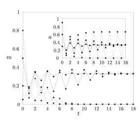
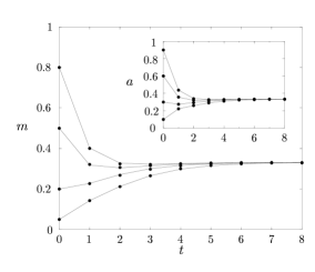
Figure 6: Evolution of $m$ and $a$ as a function of time for sequential (bottom) and synchronous (top) updating for $\beta J=8$, $\beta K=-10$. The dots correspond to simulation points. For synchronous dynamics, the paths leading to a cycle in $a$ have been plotted with dashed lines.

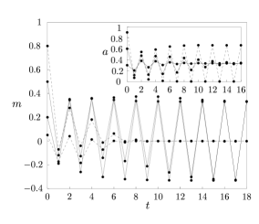
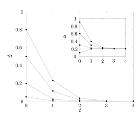
Figure 7: Evolution of $m$ and $a$ as a function of time for sequential (bottom) and synchronous (top) updating for $\beta J=-8$, $\beta K=-10$. The dots correspond to simulation points. For synchronous dynamics, the paths leading to a cycle in $a$ have been plotted with dashed lines.

The second set of points lie in region IV of the phase diagram fig. 4, i.e., $\beta J=\pm 8$ and $\beta K=-10$ and the results of the dynamics are shown in figs. 6 and 7. The dots correspond to simulations points. When $\beta J>0$ (fig. 6) we see that the sequential system (bottom) always goes to the ferromagnetic solution for any initial condition. We note that for sequential dynamics, $t=1$ corresponds to 1 update per spin in average. The synchronous system (top), however, has two minima in the free energy, and depending on the initial condition it evolves to the $m=0$ solution or to the $m>0$ ferromagnetic one. In addition, the basin of attraction is somewhat involved in the sense that the initial conditions $m(0)=0.8$ ($a=0.9$) and $m(0)=0.05$ ($a=0.1$) lead to the $m=0$ solution, while the initial conditions $m(0)=0.5$ ($a=0.6$) and $m(0)=0.2$ ($a=0.3$) lead to the ferromagnetic one. The behaviour in $a$ is as expected: when $m$ reaches the ferromagnetic solution, $a$ tends to a single finite value, while when $m=0$, $a$ enters a two-cycle. Indeed we are in the region of the phase diagram where three solutions for $a$ are allowed (recall fig. 4). For the sake of clarity, we have only included one of the cycles in $a$ for the synchronous updating figures (the one for $m(0)=0.8$, $a(0)=0.9$)

When $\beta J<0$ (fig. 7) the sequential system always evolves to the $m=0$ solution, while the synchronous one shows a similar behaviour as in fig. 6, the only difference being that now the ferromagnetic solution is a two-cycle in $m$.

6 Concluding remarks

In this paper we have studied some of the physical consequences of the way spins are updated, sequentially respectively synchronously, in classical multi-state Ising-type spin systems. First, we have derived the general form of the (pseudo-) Hamiltonian for $Q$-Ising and Blume-Emery- Griffiths (BEG) spin-glasses with synchronous updating on the basis of detailed balance.

Next, in order to study the precise differences in the stationary behaviour we have chosen to simplify these models to $Q$-Ising and BEG (anti-) ferromagnets, on the one hand because these are exactly solvable both through a free-energy analysis and a functional integration approach and on the other hand because we did not find these results in the literature.

In the case of the $Q=3$ Ising model, no surprising behaviour has been found in the sense that the phase diagram for synchronous updating is symmetric with respect to the zero-coupling axis $J=0$, and that the same stationary solutions appear as for sequential updating except for negative couplings where cycles of period two in $m$ occur in the ferromagnetic phase.

The differences in the behaviour of the BEG (anti)-ferromagnet are partly unexpected. Whereas the phase diagram for sequential updating is even simpler than the corresponding one for the $Q=3$ Ising model, a much richer phase diagram appears in the case of synchronous updating. Symmetry with respect to the axis $J=0$ still persists in this case, but the presence of a second relevant order parameter allows for much richer behaviour. The region of negative $K$ coupling is characterized by a more complicated free energy landscape. For instance, when $\beta K$ is sufficiently negative three paramagnetic solutions exist with different values for the spin activity, two-cycles in $a$ appear in different regions of the parameter space and a coexistence region of the ferromagnetic and paramagnetic solutions is found for certain values of the coupling parameters. When looking at the Hamiltonian of the BEG system, one expects the most interesting behaviour in the region $J>0$, $K<0$ (also $J<0$ for synchronous dynamics), since both terms in the Hamiltonian favour different states for the spins. Moreover, the fact that for synchronous dynamics one has to work with two types of spins makes the picture still more involved.

These findings suggest that also in more complicated disordered spin systems like the BEG spin-glass or neural network the differences between sequential and synchronous updating might be much richer and more interesting than one expects.

References

- (1) I. Pérez Castillo and N.S. Skantzos The Little-Hopfield model on a Random graph, cond-mat/0309655
- (2) N.S. Skantzos and A.C.C. Coolen, J. Phys. A 33, (2000) 1841
- (3) P. Peretto, Biol. Cybern. 50, (1984) 51
- (4) N.S. Skantzos and A.C.C. Coolen, J. Phys. A 33, (2000) 5785
- (5) J.F. Fontanari and R. Köberle, J. Phys. France 49, (1988) 13
- (6) D. Sherrington and S. Kirkpatrick, Phys. Rev. Lett. 35, (1972) 1792
- (7) H. Nishimori, 1997 TITECH technical report, unpublished
- (8) H. Rieger, J. Phys. A 23, (1990) L1273
- (9) S.K. Ghatak and D. Sherrington, J. Phys. C 10, (1977) 3149
- (10) H.W. Capel, Physica 32, (1966) 966; M. Blume, Phys. Rev. 141, (1966) 517; M. Blume, V.J. Emery and R.B. Griffiths, Phys. Rev. A 4, (1971) 1071
- (11) J.M. de Araújo, F.A. da Costa and F.D. Nobre, Eur. Phys. J. B 14, (2000) 661
- (12) A. Crisanti and L. Leuzzi, Thermodynamic Properties of a Full-Replica-Symmetry-Breaking Ising Spin Glass on Lattice Gas: the Random Blume-Emery-Griffiths-Capel Model, Physical Review B , (2004) in press, cond-mat/0402243
- (13) D.R.C. Dominguez and E. Korutcheva, Phys. Rev. E 62, (2000) 2620
- (14) D. Bollé and T. Verbeiren, Physics Letters A 297, (2002) 156
- (15) D. Bollé, in Advances in condensed matter and statistical mechanics, eds. E. Korutcheva and R. Cuerno, Nova Science Publishers (New York, 2004), p. 319
- (16) A.C.C Coolen, in Handbook of Biological Physics, Vol.4 ed. F. Moss and S. Gielen, Elsevier Science B.V., 2001, p. 531.
- (17) P.C. Martin, E.D. Siggia, and H.A. Rose, Phys. Rev. A 8, (1973) 423
- (18) A.C.C Coolen, in Handbook of Biological Physics, Vol.4 ed. F. Moss and S. Gielen, Elsevier Science B.V., 2001, p. 597.
- (19) D. Bedeaux, K. Lakatos-Lindenberg and K. Shuler, J. Math. Phys. 12, (1971) 2116