Soft annealing: A new approach to difficult computational problems
Nicolas Sourlas

Laboratoire de Physique Théorique de l’Ecole Normale Supérieure ,

24 rue Lhomond, 75231 Paris CEDEX 05, France

ABSTRACT

I propose a new method to study computationally difficult problems. I consider a new system, larger than the one I want to simulate. The original system is recovered by imposing constrains on the large system. I simulate the large system with the hard constrains replaced by soft constrains. I illustrate the method in the case of the ferromagnetic Ising model and in the case the three dimensional spin-glass model. I show that in both models the phases of the soft problem have the same properties as the phases of the original model and that the softened model belongs to the same universality class as the original one.

I show that correlation times are much shorter in the larger soft constrained system and that it is computationally advantageous to study it instead of the original system.

This method is quite general and can be applied to many other systems.

It is well known that there exists a large class of systems which are particularly hard to study both analytically and numerically. Such systems are found in condensed matter physics (spin glasses, random field models and more generally disordered systems) but also in combinatorial optimization problems or in communication theory (error correcting codes). The common future of those systems is the existence of a large number of local minima, separated by large barriers. The simulation algorithm gets trapped in those minima.

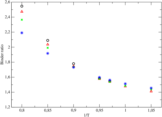
Figure 1: Binder ratio $r$ plotted as a function of $\beta=1/T$. Black circles represent data for linear size $L=16$, red triangles for $L=14$, green $x$’s for $L=12$ and blue stars for $L=8$.

In this paper I propose a new method, I call soft annealing, in which I enlarge the space on which the original system is defined. The original system is recovered by imposing constrains on the large system. I propose to simulate the large system with the hard constrains replaced by soft constrains. By enlarging the space on which the problem is defined, it is hoped that one can get around the barriers and speed up the dynamics of the algorithm, while retaining all the essential properties of the system. This is known to be the case for error correcting codes[1]. I will show that this is also the case for spin glasses and that it is advantageous to study the large system.

I will illustrate the method with the example of spin models in three dimensional cubic lattices, but the method is more general.

Consider a spin model described by the Hamiltonian

$$-H^{0}=\sum_{x,y,z=1}^{L}J^{x}(x,y,z)\sigma(x,y,z)\sigma(x+1,y,z)+J^{y}(x,y,z)\sigma(x,y,z)\sigma(x,y+1,z)$$

$$+J^{z}(x,y,z)\sigma(x,y,z)\sigma(x,y,z+1)$$

where the $\sigma$’s are Ising spins on a cubic lattice of linear size $L$.

Now consider the following new Hamiltonian:

$$-H^{new}=\sum_{x,y,z=1}^{L}J^{x}(x,y,z)\sigma^{x}(x,y,z)\sigma^{x}(x+1,y,z)+J^{y}(x,y,z)\sigma^{y}(x,y,z)\sigma^{y}(x,y+1,z)$$

$$+J^{z}(x,y,z)\sigma^{z}(x,y,z)\sigma^{z}(x,y,z+1)+$$

$$u(\sigma^{x}(x,y,z)\sigma^{y}(x,y,z)+\sigma^{x}(x,y,z)\sigma^{z}(x,y,z)+\sigma^{y}(x,y,z)\sigma^{z}(x,y,z))$$

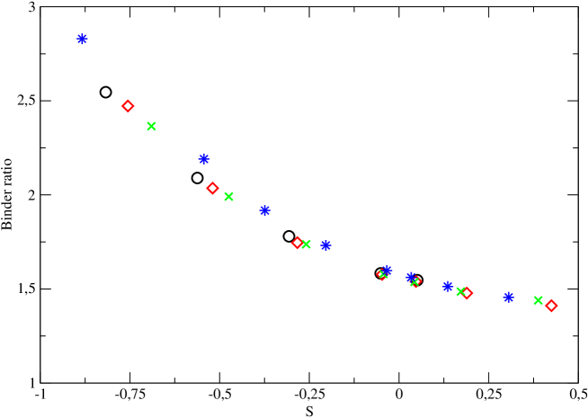
Figure 2: Binder ratio $r$ plotted versus the scaling variable $s$ (see text). Black circles represent data for linear size $L=16$, red squares for $L=14$, green $x$’s for $L=12$ and blue stars for $L=8$.

$H^{new}$ contains three times more spins than $H^{0}$. To every $\sigma(x,y,z)$ of the original Hamiltonian $H^{0}$ correspond the three spins $\sigma^{x}(x,y,z)$, $\sigma^{y}(x,y,z)$ and $\sigma^{z}(x,y,z)$. $\sigma^{x}(x,y,z)$ is coupled to its near neighboring spins in the direction $x$, $\sigma^{y}(x,y,z)$ in the direction $y$ and $\sigma^{z}(x,y,z)$ in the direction $z$. The ferromagnetic coupling $u$ couples together the three types of spin on every lattice site. For $u=0$ $H^{new}$ reduces to $3L^{2}$ decoupled one dimensional chains. For $u\to\infty$, $\sigma^{x}(x,y,z)=\sigma^{y}(x,y,z)=\sigma^{z}(x,y,z)$ and $H^{new}$ reduces to $H^{0}$. I will call the model described by $H^{new}$ the soft constrained model and the original model described by $H^{0}$ the hard constrained model.

If $H^{0}$ has a phase transition at $\beta=1/T=\beta_{c}$, we expect the phase diagramme of $H^{new}$ to be two dimensional. For small $u$, $H^{new}$ is essentially one dimensional and there is no phase transition. For $\beta<\beta_{c}$ there is again no phase transition, irrespectively of the value of $u$. In general, for $\beta<\beta_{c}$, there will be a line in the $\beta=1/T$, $v=u\beta$ plane, separating the high temperature from the low temperature phase. We expect the points along this critical line to be on the same universality class, i.e. the critical exponents to remain the same, and equal to their value in the model described by $H^{0}$ i.e. the $u\to\infty$ limit.

First I verified that all this is true in the case of the ferromagnetic Ising model in 3 dimensions. It is known that in this case $\beta_{c}\sim.22$ . I simulated $H^{new}$ for $\beta=.25$ and different values of $v$. I found a ferromagnetic to paramagnetic phase transition for $v=v_{c}=.794\pm.005$. By finite size scaling I checked that the critical exponents $\nu$ and the magnetic susceptibility exponent are compatible with the best known values for the 3 dimensional Ising model.

Much more interesting is the case of the spin glass model because it is well known to be computationally hard. I simulated the Edwards Anderson model on a cubic lattice with periodic boundary conditions. The couplings $J$ are independent random variables taking the values $\pm 1$ with equal probability. This model has been studied a lot (for a review see reference[2]). It undergoes a phase transition for $\beta=.90$ and the value of the critical exponent $\nu$ is $\nu=1.7\pm.3$[3].

I studied the soft version of this model for different values of $\beta$, keeping the ratio $u=v/\beta$ fixed to $u=.75$ and for the lattice sizes $L=8,\ 12,\ 14$ and $L=16$. For every size I simulated 1280 realizations of the couplings. For every realization of the couplings I simulated two copies $\sigma$ and $\tau$ and studied the probability distribution of the overlap $q$[4]

$$q=({1\over{3L^{3}}})\sum_{x,y,z}(\sigma^{x}(x,y,z)\tau^{x}(x,y,z)+\sigma^{y}(x,y,z)\tau^{y}(x,y,z)+\sigma^{z}(x,y,z)\tau^{z}(x,y,z))$$ (1)

I measured the Binder ratio $r(\beta,L)={\overline{<q^{4}>}}/({\overline{<q^{2}>}})^{2}$ where, as usually, $\overline{a}$ is the average of $a$ over the coupling samples, and the results are shown in figure 1. The data for the different sizes cross at $\beta=.96\pm.05$. This shows that there is a phase transition for $\beta=\beta_{c}=.96\pm.05$. Figure 2 shows the same data plotted versus the scaling variable $s=(\beta-\beta_{c})L^{1/\nu}$ with $\nu=1.7$, the exponent of the Edwards-Anderson model[3]. We see that the data for the different sizes collapse on the same curve except maybe for the $L=8$ data which seem to be slightly apart, which indicates corrections to scaling for $L=8$. The value $r_{c}$ of $r$ at $\beta=\beta_{c}$ is an universal quantity, sometimes called the renormalized coupling constant. We find $r_{c}=1.53\pm.03$. For the original model $r_{c}\sim 1.5$[3]. So our results are compatible with both the exponent $\nu$ and the renormalized coupling constant $r_{c}$ taking the same value in the soft model and in the original Edwards-Anderson model. We conclude that the hypothesis that the two models belong to the same universality class is supported by our data.

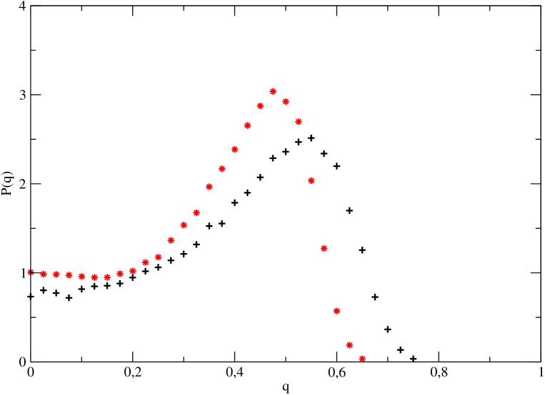
Figure 3: Average probability distribution $P(q)$ of the overlaps $q$ for $\beta=1.05$ and sizes $L=14$ (stars in red) and $L=8$ (crosses in black).

Figure 3 shows the probability distribution of the overlaps $P(q)$ averaged over the samples for $\beta=1.05$ and for the two sizes $L=8$ and $L=14$. The similarity with the $P(q)$ of the hard constrained model[3] is striking. $P(q)$ has a peack at a value of $q$ we call $q_{EA}$. As the volume increases, the peack is sharper and $q_{EA}$ decreases, as in the original Edwards Anderson model. I measured also the link-link overlap $q_{e}$ of two real replicas $\sigma$ and $\tau$, $q_{e}=(1/3L^{3})\sum_{i,j}\sigma_{i}\sigma_{j}\tau_{i}\tau_{j}$ (the sum runs over the nearest neighbor sites of the lattice) and the joined probability distribution, $P(q,q_{e})$ averaged over the samples. I found that $P(q,q_{e})$ is very peacked around a line $q_{e}=e_{0}+e_{1}q^{2}+e_{2}q^{4}$, with $e_{0}\sim.54$, $e_{1}\sim.10$ and $e_{2}\sim.30$. The $e_{i}$’s are to a good approximation $L$ independent. I measured the variance $w^{2}={\overline{<(q_{e}-e_{0}-e_{1}q^{2}-e_{2}q^{4})^{2}>}}$. I found for $\beta=1.05$ $w^{2}=.0004$ for $L=8$, $w^{2}=.00015$ for $L=12$, $w^{2}=.0001$ for $L=14$, and $w^{2}=.00008$ for $L=16$, i.e. when the volume increases $P(q,q_{e})$ goes to a delta function $P(q,q_{e})=P(q)\delta(q_{e}-e_{0}+e_{1}q^{2}+e_{2}q^{4})$ This is the case in the infinite range model and in the case of the hard constrained model[5, 6, 7]. We conclude that the hard and soft constrained models belong to the same universality class and that their low temperature phases are extremely similar.

We expect the soft model to be easier to simulate numerically. To verify this one usually measures the spin autocorrelation functions, averaged over the samples,

$$C^{h}(t)=(1/L^{3})\sum_{i}{\overline{<\sigma_{i}(t_{0})\sigma_{i}(t_{0}+t)>}}$$

and

$$C^{s}(t)=(1/3L^{3}){\overline{<\sum_{i}\sigma_{i}^{x}(t_{0})\sigma_{i}^{x}(t_{0}+t)+\sigma_{i}^{y}(t_{0})\sigma_{i}^{y}(t_{0}+t)+\sigma_{i}^{z}(t_{0})\sigma_{i}^{z}(t_{0}+t)>}}$$

for the hard and soft constrained models respectively, where $t$ is the number of Monte Carlo sweeps over the lattice. I compared $C^{h}(t)$ and $C^{s}(t)$ each one measured at the critical value of $\beta$, $\beta_{c}^{h}=.90$ for $C^{h}(t)$ and $\beta_{c}^{s}=.97$ for $C^{s}(t)$. They are plotted in figure 4.

There are three curves in figure 4.

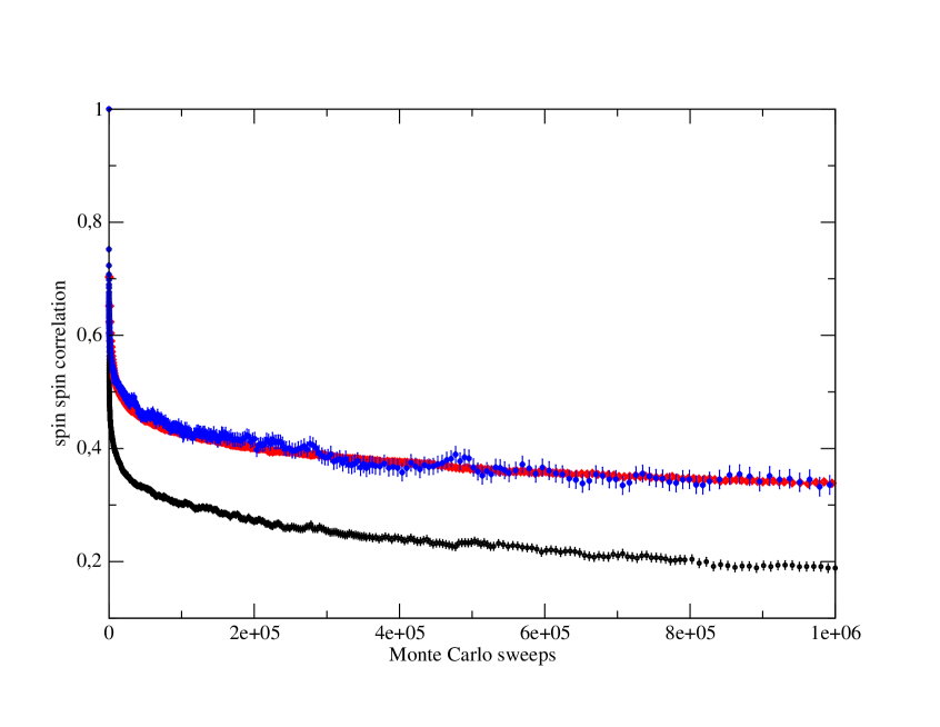
Figure 4: Spin-spin autocorrelations $C^{h}(t)$ and $C^{s}(t)$ at $\beta^{h}_{c}$ and $\beta^{s}_{c}$ (see text) as a function of the number of the lattice Monte Carlo sweeps.

The lower curve (in black) corresponds to $C^{s}(t)$. It is difficult to distinguish between the two other curves because they fall on top of each other. One of the two, the curve in blue, corresponds to $C^{h}(t)$. We see that $C^{s}(t)$ indeed decays much faster than $C^{h}(t)$. In order to make the comparison more quantitative, I plotted also in figure 4 $C^{s}(wt)$ (the curve in red), i.e. I rescaled the “time” in $C^{s}(t)$ by an appropriated scaling factor $w$. We see that, with this rescaling, $C^{s}(wt)$ and $C^{h}(t)$ can be made to coincide.

The scaling factor $w$ was chosen as follows. $C^{s}(t)$ and $C^{h}(t)$ are decreasing functions of $t$ and $C^{s}(0)=C^{h}(0)=1$. I measure the number of lattice sweeps $t^{h}(c,\beta)$ and $t^{s}(c,\beta)$ needed for $C^{s}$ and $C^{h}$ fall below the value $c$, i.e. $C^{h}(t^{h}(c,\beta))=c$ and $C^{s}(t^{s}(c,\beta))=c$. For $c=.40$ and $L=12$ I found that the time ratio $r_{t}^{critical}(c=.40)=t^{h}(.40,\beta_{c}^{h})/t^{s}(.40,\beta_{c}^{s})\sim 28$. In figure 4 I chose $w=r_{t}^{critical}(c=.40)$. We see that with this rescaling of the Monte Carlo time, the spin autocorrelation functions coincide for all $1\leq t\leq 10^{6}$, i.e. one has to perform 28 times more lattice sweeps for the hard constrained system in order for the spins to de-correlate the same amount as for the soft system. In order to study the size dependence of this difference of the correlation times, I measured $r_{t}^{critical}(c=.40)$ for $L=8$ and $L=16$. I found that $r_{t}^{critical}(c=.40)=7.7$ for $L=8$ and $r_{t}^{critical}(c=.40)=39$ for $L=16$, i.e. $r_{t}^{critical}$ (and therefore the gain in simulation time) strongly increases with lattice size. It is not clear yet whether $r_{t}^{critical}$ obeys some kind of finite size scaling.

I conclude that, by softening the constrains, the gain in computer time is large, despite the fact that the number of spins in $H^{new}$ is larger by a factor of three. This gain icreases with the size of the system.

The method of softening the constrains presented here is obviously not unique. For example one could consider

$$H^{\prime}=\sum_{i,j}J_{i,j}X{i,j}+u\sum_{plaquettes}X_{i,j}X_{j,k}X_{k,l}X_{l,i}$$

The term proportional to $u$ runs over all the plaquettes, i.e. the elementary squares, of the lattice. $X_{i,j}$ corresponds to $\sigma_{i}\sigma_{j}$ of the original Hamiltonian and the coupling $u$ imposes the constrain $X_{i,j}X_{j,k}X_{k,l}X_{l,i}=\sigma_{i}\sigma_{j}\sigma_{j}\sigma_{k}\sigma_{k}\sigma_{l}\sigma_{l}\sigma_{i}=1$ One of the advantages of the method used in this paper is that all the techniques which speed up simulations like multi-spin coding and parallel tempering can easily be implemented in the soft model.

I have illustrated the method with the notoriously difficult example of the three dimensional spin glass model. It would be interesting to apply this method also to other difficult optimization problems.

I would like to thank Andrea Montanari for several discussions.

References

- [1] For a review of the Statistical Mechanics of error correction codes see N. Sourlas in The Physics of Communication, Proceedings of the XII Solvay Conference on Physics, edited by I. Antoniou, V.A. Sadovnichy and H. Walther (World Scientific, Singapore, 2003).
- [2] E. Marinari, G. Parisi and J.J. Ruiz-Lorenzo, in Spin Glasses and Random Fiels, edited by A.P. Young (World Scientific, Singapore, 1998).
- [3] N. Kawashima and A.P. Young, Phys. Rev. B 53 R484 (1996).
- [4] G. Parisi Phys. Rev. Lett., 24 1946 (1983)
- [5] S. Caracciolo, G. Parisi, S. Patarnello and N. Sourlas, Europhys. Lett. , 11 783 (1990)
- [6] S. Caracciolo, G. Parisi, S. Patarnello and N. Sourlas, J. Phys. France, 51 1877 (1990)
- [7] Enzo Marinari and Giorgio Parisi, Phys. Rev. Lett. 86 3887 (2001).