A generalized approach to complex networks

Abstract

This work describes how the formalization of complex network concepts in terms of discrete mathematics, especially mathematical morphology, allows a series of generalizations and important results ranging from new measurements of the network topology to new network growth models. First, the concepts of node degree and clustering coefficient are extended in order to characterize not only specific nodes, but any generic subnetwork. Second, the consideration of distance transform and rings are used to further extend those concepts in order to obtain a signature, instead of a single scalar measurement, ranging from the single node to whole graph scales. The enhanced discriminative potential of such extended measurements is illustrated with respect to the identification of correspondence between nodes in two complex networks, namely a protein-protein interaction network and a perturbed version of it. The use of other measurements derived from mathematical morphology are also suggested as a means to characterize complex networks connectivity in a more comprehensive fashion.

I Introduction

One of the unavoidable consequences of the fast pace of developments in the new area of complex networks Albert and Barabási (2002); Dorogovtsev and Mendes (2002, 2003); Newman (2003) is that, while many impressive and relevant concepts and perspectives have been identified and well-developed, and promising results been obtained, some interesting issues have received relatively little attention. One particularly important point is the fact that, despite the major advances achieved by using powerful tools from theoretical physics (e.g. Albert and Barabási (2002); Newman (2003)), relatively little attention has been given to the treatment of complex networks in terms of discrete mathematics and mathematical morphology, which are themselves well-established investigation fields. Developed mainly by J. Serra and collaborators Serra (1984) , the area of mathematical morphology is aimed, through strict mathematical formalization, at representing and analyzing the geometrical and topological features of discrete mathematical structures, especially regular lattices such as those underlying digital images da F. Costa and Jr (2001). Mathematical morphology is strongly founded on the discrete operations of complement, dilation and erosion, which can be composed in order to obtain a whole series of new operators with specific properties. At the same time, previous developments by L. Vincent and H. Heijmans Vincent (1989); Heijmans et al. (1992) have shown how the mathematical morphology framework can be extended to graphs, allowing not only the precise mathematical representation and manipulation of those general structures, but also the immediate access to the wealthy of existing results from mathematical morphology.

The present article reports on how the application of discrete mathematics, especially mathematical morphology Serra (1984) and distance-oriented concepts Vincent (1989); Heijmans et al. (1992); da F. Costa and Jr (2001), bears the potential not only for formalization, but also to obtain a series of new concepts and results. In particular, by considering the dilations of subnetworks of a network $\Gamma$ and extending the concepts of numbers of neighbors Faloutsos et al. (1999a, b); Newman (2001); Cohen et al. (2003) and hierarchical node degree Costa (2004), we show that the traditional concepts of node degree and clustering coefficient Albert and Barabási (2002); Newman (2003) can be generalized in two important ways. First, the concept of subnetwork dilation paves the way to generalize the degree and clustering coefficient to any subnetwork of $\Gamma$, and not only their specific nodes as adopted in the complex network literature. Such a concept therefore allows us to speak of the degree of subgraphs of special interest, such as cycles, sets of hubs, or the maximum spanning tree of a given complex network. Second, the consideration of a series of subsequent dilations, together with the respectively induced distance transform and rings, allow the further extension of the degree and clustering coefficient so that a signature, instead of the single scalar traditional measurements, is obtained which can provide information about the network connectivity from the node to the whole graph scales.

The potential of such hierarchical extensions for discriminating the connectivity around each node (or subgraph) can be readily appreciated by considering the fact that several nodes in a complex network will have the same degree and clustering coefficient, but very few nodes will share such values calculated for a series of subsequent neighborhoods. Such an interesting feature of the generalized measurements is illustrated in the present article with respect to protein-protein interaction networks.

II Basic Concepts

A network $\Gamma$ without multiple edges is a discrete structure composed of a set of nodes $V(\Gamma)$ and a set $E(\Gamma)$ of edges $(u,v)$ established between specific pairs of nodes of $V(\Gamma)$, so that the network $\Gamma$ is represented as $\Gamma=(V,E)$. As we consider undirected networks without loops, it follows that $(u,v)\iff(v,u)$ and $(u,u)\notin E(\Gamma)$. Such a network can be conveniently represented in terms of its respective adjacency matrix $K$ such that each edge $(u,v)$ is represented by making $K(u,v)=K(v,u)=1$, while the absence of edge is indicated by zero value. A subnetwork $\xi$ of $\Gamma$ is any network such that $V(\xi)\subseteq V(\Gamma)$ and $E(\xi)\subseteq\left\{(u,v)|(u,v)\in E(\Gamma)\>and\>u,v\in V(\xi)\right\}$. Figure 1(a) illustrates a network $\Gamma$ and one of its many subnetworks $\xi$, identified by the wider-border nodes and wider edges. Particularly interesting subnetworks of a network $\Gamma$ include its hubs, outmost nodes (i.e. nodes with low degree), as well as its cycles. Special cases of subnetworks of $\Gamma$ include the empty network $(V=\emptyset,E=\emptyset)$, where $\emptyset$ stands for the empty set, networks containing an isolated node $u$ $\Gamma_{u}=(V=\left\{u\in V(\Gamma)\right\},E=\emptyset)$, and the own original network $\Gamma$.

The complement of a subnetwork $\xi$ of $\Gamma$ is the subnetwork $\xi^{\prime}_{\Gamma}$ of $\Gamma$ such that $V(\xi^{\prime}_{\Gamma})=\left\{u|u\in V(\Gamma)\>and\>u\notin V(\xi)\right\}$ and $E(\xi^{\prime}_{\Gamma})=\left\{(u,v)|(u,v)\in E(\Gamma)\>and\>u,v\in V(\xi^{\prime}_{\Gamma})\right\}$. Figure 1(b) illustrates the complement $\xi^{\prime}_{\Gamma}$ of $\xi$ in $\Gamma$. A subnetwork is connected if any of its nodes can be reached from any of its other nodes. Two subnetworks $\zeta$ and $\xi$ of $\Gamma$ are connected if it is possible to reach a node of $\xi$ from a node of $\zeta$, and vice-versa. The maximal connected subnetworks, in the sense of including the largest number of nodes, of a network are called connected components. The subnetwork in Figure 1(a) is not connected but contains two connected components.

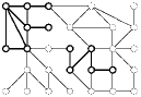
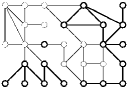
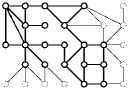
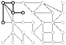
(a)                                (b)                                (c)                                (d)

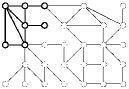
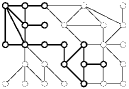
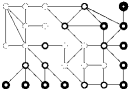
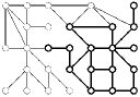
(e)                                (f)                                (g)                                (h)

Figure 1: Original network containing a subnetwork (a), identified by wider-border nodes, and its respective complement (b), dilation (c), erosion (d), opening (e), closing (f), and distance transform (g), with the distances identified by the node border width. The generalized Voronoi tessellation of the two connected components of the subnetwork in (a) is shown in (h). 

The degree of a node $u$ of $\Gamma$, hence $k(u)$, corresponds to the number of edges attached to that node. The degree of a subnetwork $\xi$ of $\Gamma$, hence $k(\xi)$, is defined as the number of edges implied by the dilation of $\xi$, i.e. those edges connecting $\xi$ to the rest of $\Gamma$. For instance, the degree of the subnetwork $\xi$ in Figure 1(a) is 12. The outmost set of a subnetwork $\xi$ of $\Gamma$ is the set of nodes $\Omega(\xi)$ which have unit degree. For simplicity’s sake, such nodes are henceforth referred to as outnodes. The 1-neighborhood of a node $u$ of $\Gamma$, henceforth represented as $n_{1}(u)$, is the set of nodes of $\Gamma$ which are attached to $u$, plus node $u$. This concept can be immediately extended to express the neighborhood of a subnetwork $\xi$ of $\Gamma$, given as the set of nodes of $\Gamma$ which are connected to $\xi$ plus the nodes in $V(\xi)$.

III Complex Network Morphology

The dilation of a subnetwork $\xi$ of $\Gamma$ is defined as the subnetwork $\delta(\xi)$ of $\Gamma$ having $V(\delta(\xi))=n_{1}(\xi)$ as its set of nodes while its set of edges include the edges of $\Gamma$ found between the nodes in $n_{1}(\xi)$. The erosion of $\xi$, represented as $\varepsilon(\xi)$, is a subnetwork of $\Gamma$ which can be defined as the complement of the dilation of $\xi^{\prime}_{\Gamma}$, i.e. $\varepsilon(\xi)=(\delta(\xi^{\prime}_{\Gamma}))^{\prime}_{\Gamma}$. Observe that the dilation or erosion of $\Gamma$ yields $\Gamma$ as result. Figures 1(c) and (d) ilustrates the dilation and erosion of the subnetwork $\xi$ in (a), respectively. Observe that the erosion eliminated one of the connected components of $\xi$. Generally, $\delta(\varepsilon(\xi))\neq\varepsilon(\delta(\xi))$, i.e. the dilation can not be used to undo an erosion, and vice-versa. Observe also that a subnetwork $\xi$ is necessarily contained or equal to its respective dilation, while the erosion of a subnetwork $\xi$ is necessarily contained or equal to itself.

The d-dilation of a subnetwork $\xi$ is defined as the subnetwork obtained by dilating $d$ times the subnetwork $\xi$, i.e.:

$$\delta_{d}(\xi)=\underbrace{\delta(\delta(\ldots(\xi)\ldots))}_{d}$$ (1)

Similarly, the d-erosion can be defined as:

$$\varepsilon_{d}(\xi)=\underbrace{\varepsilon(\varepsilon(\ldots(\xi)\ldots))}_{d}$$ (2)

Observe that $\delta_{d}(\xi)$ converges to $\Gamma$ as $d$ is increased, while $\varepsilon_{d}(\xi)$ converges to the empty network under similar circumstances. We also have that $\delta_{d=i+j}(\xi)=\delta_{i}(\delta_{j}(\xi))=\delta_{j}(\delta_{i}(\xi))$ and $\varepsilon_{d=i+j}(\xi)=\varepsilon_{i}(\varepsilon_{j}(\xi))=\varepsilon_{j}(\varepsilon_{i}(\xi))$. The d-degree of a subnetwork $\xi$ is defined as the degree of the d-dilation of the network $\xi$, i.e., $k_{d}(\xi)=k(\delta_{d}(\xi))$.

It is possible to use combinations of dilations and erosions of a subnetwork $\xi$ in order to obtain new operators such as the opening and closing of $\xi$, which are defined as $\alpha(\xi)=\delta(\varepsilon(\xi))$ and $\omega(\xi)=\varepsilon(\delta(\xi))$, respectively. Figures 1 (e) and (g) illustrate, respectively, the opening and closing of the subnetwork $\xi$ in (a). Observe that the closing of $\xi$ had as an effect the connection of the two components of that subnetwork, filling the gap between those subnetworks. The opening and closing operations are idempotent, in the sense that $\alpha(\alpha(\xi))=\alpha(\xi)$ and $\omega(\omega(\xi))=\omega(\xi)$. It is also interesting to define the d-opening of a subnetwork $\xi$, henceforth represented as $\alpha_{d}(\xi)$, corresponding to $d$ erosions followed by $d$ dilations. The d-closing of $\xi$, represented as $\omega_{d}(\xi)$ can be defined in similar fashion. The latter operator is useful for investigating the progressive merging of subnetworks of $\Gamma$ in terms of increasing values of $d$. Particularly, interesting information about the network structure can be provided by the evolution of the number of connected subnetworks, starting from a specific set $\chi$ of subnetworks (e.g. the network 3-cycles), in terms of a sequence of d-openings (or closings) performed for increasing values of $d$.

IV Distances, Distance Transforms, Parallels and Rings

Several important features of a complex network are related to the concept of distance. If $\zeta$ and $\xi$ are any subnetworks of $\Gamma$, the (minimal) distance between the respective set of nodes $V(\zeta)$ and $V(\xi)$, hence $D(V(\zeta),V(\xi))$, can be defined as the value of $d$ for which some node $u$ of $\zeta$ becomes included into $V(\delta_{d}(\xi))$. It can be verified that $D(V(\zeta),V(\xi))=D(V(\xi),V(\zeta))$. Observe that $D(V(\zeta),V(\zeta))=0$. In particular, the distance between a node $u$ and a subnetwork $\xi$ is given as $D(\{u\},V(\xi))$. The distance transform of a subset of nodes $\chi$ of $\Gamma$ is the mapping which assigns $D(\{u\},\chi)$ to every node $u\in V(\Gamma)$, including those in $\xi$. Figure 1(g) illustrate the distance transform of the subnetwork in (a), with the distance values (4 values for this subnetwork, i.e. $d=0,1,2,$ and $3$) expressed in terms of the node borders widths. Given a subnetwork $\xi$ of $\Gamma$, the subnetwork $\varrho$ defined by the set $V(p)$ of nodes such that $D(V(\varrho),V(\xi))=d$ and the set of those edges of $\Gamma$ connecting nodes in $V(\varrho)$ is called the d-parallel of $\xi$, henceforth represented as $P_{d}(\xi)$. The parallels of the subnetwork $\xi$ in Figure 1(a) correspond to the set of nodes with the same width in (g) plus the respective interconnecting edges. The number of nodes and edges in a d-parallel of $\xi$ are henceforth represented as $n\{P_{d}(\xi)\}$ and $e\{P_{d}(\xi)\}$. Similarly, it is interesting to define the rs-ring of $\xi$, hence $R_{rs}(\xi)$, which corresponds to the union of the respective parallels of $\xi$ for distances $d=r$ to $s$ plus the edges of $\Gamma$ interconnecting such parallels. The number of nodes and edges in a rs-ring of $g$ are henceforth represented as $n\{R_{rs}(\xi)\}$ and $e\{R_{rs}(\xi)\}$. Observe that a d-parallel therefore is the particular case of the rs-ring for $d=r=s$. Another interesting possibility is to use the above introduced distance concepts in order to obtain the generalized Voronoi tessellation of subnetworks, as illustrated in Figure 1(h) with respect to the two connected components in the subnetwork in Figure 1(a).

The above definitions allow the concept of clustering coefficient Albert and Barabási (2002); Newman (2003) to be generalized to parallels and rings of any subnetwork. The rs-clustering coefficient of a subnetwork $\xi$ of $\Gamma$, henceforth represented as $cc_{rs}(\xi)$, can be defined as the number of edges in the respective rs-ring subnetwork, divided by the total of possible edges between the nodes in that ring, i.e.:

$$cc_{rs}(\xi)=\frac{2e\{R_{rs}(\xi)\}}{n\{R_{rs}(\xi)\}(n\{R_{rs}(\xi)\}-1)}$$ (3)

V Hierarchical Measurements for Single Nodes

The concepts discussed above can be naturally extended to a single node and to an edge, respectively, whether the subgraph contains the node alone and whether the subgraph contains the edge and both nodes connected by the edge da F. Costa (2005); L. da F. Costa and Boas (2005). Using the concept of rings considered in the last section, henceforth the subgraph $\zeta$ composed of the ring $R_{d}(u)$ is defined as the hierarchical level related to the subgraph $\xi$ composed of the single node $(u)$, such that, the hierarchical number of nodes $n_{d}(u)$ (or $n\{R_{d}(u)\}$) is given as the number of nodes at hierarchical distance $d$ from de reference node $(u)$, i.e., the number of nodes in the ring $R_{d}(u)$. Hence, the hierarchical degree $k_{d}(u)$ is defined as the number of edges between the nodes in the ring $R_{d}$ and $R_{d+1}$, such that the hierarchical number of edges among the nodes in the ring $R_{d}(u)$ is $e_{d}(u)$ (or $e\{R_{d}(u)\}$). The hierarchical clustering coefficient $cc_{d}(u)$ is written using equation 3.

$$cc_{d}(u)=\frac{2e_{d}(u)}{n_{d}(u)(n_{d}(u)-1)}$$ (4)

At last, other hierarchical measurements can be derived from the above definitions and each of them will be dealt with in turn:

• Convergence ratio $(C_{d}(u))$ : Measures the ratio between the hierarchical node degree of node $(u)$ at hierarchical distance $d-1$ and the hierarchical number of nodes in the ring $R_{d}(u)$.

  $$C_{d}(u)=\frac{k_{d-1}(u)}{n_{d}(u)}$$ (5)

• Intra-ring degree $(A_{d}(u))$ : The average among the degrees of the nodes in the ring $R_{d}(u)$.

  $$A_{d}(u)=\frac{2e_{d}(u)}{n_{d}(u)}$$ (6)

• Inter-ring degree $(E_{d}(u))$ : The average of the number of connections between each node in ring $R_{d}(u)$ and those in $R_{d+1}(u)$.

  $$E_{d}(u)=\frac{k_{d}(u)}{n_{d}(u)}$$ (7)

• Hierarchical common degree $(H_{d}(u))$ : The average node degree among the nodes in $R_{d}(u)$, considering all edges connected to nodes in the ring.

  $$H_{d}(u)=\frac{2e_{d}(u)+k_{d-1}(u)+k_{d}(u)}{n_{d}(u)}$$ (8)

A summary of the hierarchical measurements considered in the present work are presented in the table bellow.

Hier. number of nodes in the ring $R_{d}(u)$.	$\mathbf{n_{d}(u)}$
Hier. number of edges among the nodes in the ring $R_{d}(u)$.	$\mathbf{e_{d}(u)}$
Hier. degree of node $(u)$ at distance $d$.	$\mathbf{k_{d}(u)}$
Hier. clustering coefficient of node $(u)$ at hier. level $d$.	$\mathbf{cc_{d}(u)}$
Convergence ratio of node $(u)$ at hier. level $d$.	$\mathbf{C_{d}(u)}$
Intra-ring node degree of node $(u)$ at distance $d$.	$\mathbf{A_{d}(u)}$
Inter-ring node degree of node $(u)$ at distance $d$.	$\mathbf{E_{d}(u)}$
Hier. common degree of node $(u)$ at distance $d$.	$\mathbf{H_{d}(u)}$

Table 1 – Summary of the hierarchical measurements considered in this work.

VI Evaluation of Discriminative Power

Given a complex network, it is possible to organize several selected measurements of its topology into a feature vector $\overrightarrow{\mu}$ (e.g. L. da F. Costa and Boas (2005)), which therefore provides a quantitative description of properties of the network. Multivariate statistical methods (e.g. da F. Costa and Jr (2001)) can then be applied in order to separate such vectors into clusters or to identify the category of the network.

In a similar fashion, it is possible to assign a feature vector to individual nodes of the network, so that they can be characterized and organized into classes. Although simple measurements such as the node degree and clustering coefficients can be used for this purpose, they are generally not enough for a discriminative characterization of nodes at the individual level because several nodes in a large network will have identical values of such measurements. The hierarchical extensions of the node degree and clustering coefficient, combined with the ancillary hierarchical measurements described in this work, account for substantially enhanced discrimination of the local properties of the connectivity around each node, therefore diminishing the degeneracy of the description. In other words, several nodes may have the same immediate node degree, but it is rather unlikely that they will also share other hierarchical degrees. At the same time, nodes which do present similar connectivity patterns along the hierarchies can be clustered into meaningful classes by considering feature vectors composed of hierarchical measurements.

In order to illustrate the above possibilities, we considered a S. cerevisiae protein-protein interaction network $\Gamma$ Sprinzak and Margalit (2001) containing $N=1922$ nodes and without self-connections and isolated nodes. A perturbed version of this network was obtained by rewiring the edges with probability $p$. Nodes in these two networks are then characterized in terms of several combinations of hierarchical measurements. In order to quantify the discriminative power of such measurements, we repeatedly selected a node from the original network and identified among all nodes of the perturbed network the node which leads to the smallest Euclidean distance between the respective feature vectors. In case these two nodes are verified to indeed correspond one another (recall that the identity of the nodes is guaranteed because the perturbed network is derived from the original network by rewiring), we understand there has been a correct identification.

Among the several combinations of measurements, considering varying hierarchical levels, the best results were obtained for pairwise combinations of $A_{d}$, $E_{d}$, $H_{d}$ and $C_{d}$, particulalry the four situations shown in Figure 2. The diagrams in this figure depict the average $\pm$ standard deviation of the percentage of correctly identified nodes by using the identified pairs of measurements up to the hierarchical levels identified in the x-axis (varying from 1 to 19). A number of interesting features can be identified from such results. First, it is interesting to notice that the average of correct identifications undergoes the three following regimes: (i increases along the 4 or 5 initial hierarchies; (ii) stays nearly constant until about 12 hierarchical levels, and (iii) then decreases steadily. This behavior is observed for all graphs in Figure 2. The average performance increase in (i) is a direct consequence of the fact that more information about the network connectivity around each node is being taken into account. The performance plateau and decrease taking place after 4 or 5 hierarchical levels are considered for the measurements reflects a degeneration in the discriminative power of the measurements caused by the fact that most of the nodes have been considered at such hierarchical depths. Similar performances are observed for the four cases illustrated in Figure 2, with slightly better results being achieved for the measurement combinations in (a) and (d). The standard deviations values tend to follow the mean, with higher variations being observed along the plateaux.

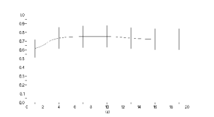
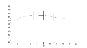
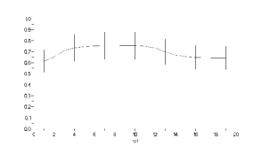
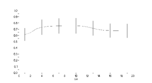
Figure 2: Four hierarchical measurements combinations for the feature vector: (a) $A_{d}$ and $E_{d}$; (b) $E_{d}$ and $H_{d}$; (c) $C_{d}$, $A_{d}$ and $H_{d}$ and (d) $A_{d}$ and $H_{d}$.

VII Concluding Remarks

This article has addressed several issues regarding the generalization of complex networks measurements. First, we have shown for the first time that complex networks and their properties can be formalized in terms of mathematical morphology, allowing the definition of a series of measurements such as the generalized versions of the node degree and clustering coefficient, as well as the possibility to use other features from mathematical morphology so as to investigate further the structure of specific subnetworks. Second, we have emphasized the importance of identifying and studying the properties of subnetworks of special interest — including the set of hubs, outnodes and 3-cycles, and shown that a particularly comprehensive study of such subnetworks can be obtained by taking into account a whole series of neighborhoods, as allowed by the the novel proposed concepts of generalized degrees and clustering coefficient.

While the new set of measurements extended to take into account subgraphs and hierarchies can be used to derive new network growth schemes and characterize and classify different types of networks, they also present power for enhanced discrimination between individual nodes. The latter has been illustrated for the first time in this article with respect to protein-protein interaction networks. More specifically, we have shown that the ability to identify correspondenced between nodes in two versions of a network (in the case of our example the original and perturbed networks) tend to increase by considering measurements taking into account multiple hierarchical levels. This is a consequence of the fact that the use of more hierarchical levels allows the measurements to reflect in a less degenerate way the network connectivity around each node.At the same time, we have shown that such enhanced discriminative power tends, with the incorporation of additional hierarchical depths, to reach a plateau and then to decrease.

The possibilities for future works include the application of the introduced concepts to community finding, characterization of resilience to attack, and extensions to measurements aimed at characterizing the assortative properties of networks.

Acknowledgments

Luciano da F. Costa is grateful to FAPESP (process 99/12765-2), CNPq (308231/03-1), NIH Fogarty, and the Human Frontier Science Program (HFSP RGP39/2002) for financial support. Luis Enrique Correa da Rocha is grateful to Human Frontier Science Program for his undergraduate grant.

References

- Albert and Barabási (2002) R. Albert and A.-L. Barabási, Reviews of Modern Physics 74, 47 (2002).
- Dorogovtsev and Mendes (2002) S. N. Dorogovtsev and J. F. F. Mendes, Advances in Physics 51, 1079 (2002).
- Dorogovtsev and Mendes (2003) S. N. Dorogovtsev and J. F. F. Mendes, Evolution of Networks, From Biological Nets to Internet and WWW (Oxford University Press, 2003).
- Newman (2003) M. Newman, SIAM Review 45, 167 (2003).
- Serra (1984) J. Serra, Image Analysis and Mathematical Morphology (Academic Press, 1984).
- da F. Costa and Jr (2001) L. da F. Costa and R. M. C. Jr, Shape Analysis and Classification: Theory and Practice (CRC Press, Boca Raton, 2001).
- Vincent (1989) L. Vincent, Signal Proc 16(4), 365 (1989).
- Heijmans et al. (1992) H. J. A. M. Heijmans, P. Nacken, A. Toet, , and L. Vincent, J. Vis. Comm. and Image Repr 3(1), 24 (1992).
- Faloutsos et al. (1999a) M. Faloutsos, P. Faloutsos, and C. Faloutsos, SIAM Review 45, 167 (1999a).
- Faloutsos et al. (1999b) C. Faloutsos, P. Faloutsos, and M. Faloutsos, Comp. Comm. Rev. 29, 251 (1999b).
- Newman (2001) M. E. Newman, cond-mat/0111070 (2001).
- Cohen et al. (2003) R. Cohen, S. Havlin, S. Mokryn, D. Dolev, T. Kalisky, and Y. Shavitt, cond-mat/0305582 (2003).
- Costa (2004) L. Costa, Phys. Rev. Lett. 93, 098702 (2004).
- da F. Costa (2005) L. da F. Costa, cond-mat/0412761 (2005).
- L. da F. Costa and Boas (2005) G. T. L. da F. Costa, F. Rodrigues and P. R. V. Boas, cond-mat/0505185. (2005).
- Sprinzak and Margalit (2001) E. Sprinzak and H. Margalit, J. Mol. Biol. 311, 681 (2001).