Response of a catalytic reaction to periodic variation of the CO pressure: Increased CO₂ production and dynamic phase transition

Abstract

We present a kinetic Monte Carlo study of the dynamical response of a Ziff-Gulari-Barshad model for CO oxidation with CO desorption to periodic variation of the CO pressure. We use a square-wave periodic pressure variation with parameters that can be tuned to enhance the catalytic activity. We produce evidence that, below a critical value of the desorption rate, the driven system undergoes a dynamic phase transition between a CO₂ productive phase and a nonproductive one at a critical value of the period and waveform of the pressure oscillation. At the dynamic phase transition the period-averaged CO₂ production rate is significantly increased and can be used as a dynamic order parameter. We perform a finite-size scaling analysis that indicates the existence of power-law singularities for the order parameter and its fluctuations, yielding estimated critical exponent ratios $\beta/\nu\approx 0.12$ and $\gamma/\nu\approx 1.77$. These exponent ratios, together with theoretical symmetry arguments and numerical data for the fourth-order cumulant associated with the transition, give reasonable support for the hypothesis that the observed nonequilibrium dynamic phase transition is in the same universality class as the two-dimensional equilibrium Ising model.

I Introduction

The study of nonequilibrium statistical models is a subject of current interest in a broad range of fields such as chemical reactions, fluid turbulence, chaos, biological populations, growth-deposition processes, and even economics general1 ; general2 . In particular, the study of surface reaction systems has received a great deal of attention surface . These systems not only constitute a fruitful laboratory for exploring critical phenomena associated with out-of-equilibrium statistical physics, but they can also play an important role in the development of more efficient catalytic processes. Catalytic reactions are widespread in nature and have many industrial and technological applications catalytic ; imbhil95 .

Several experiments show that it is possible to increase the efficiency of catalytic reactions by subjecting the system to periodic external forcing imbhil95 ; ehsasi89 ; vaporciyan88 ; cutlip83 ; hegedus80 . Monte Carlo simulations of the Ziff, Gulari, and Barshad (ZGB) model without desorption ziff86 indicate that an enhancement of the catalytic activity is observed when the system is perturbed by a periodic force that drives it briefly into the CO poisoned state ziff86 ; lopez00 . However, it is well known that the ZGB model does not reproduce several important aspects of catalytic processes, such as lateral diffusion TAMM98 and CO desorption tome93 . In the present study we neglect diffusion and concentrate on the effects of CO desorption. For brevity we will refer to this model as the ZGB-k model tome93 .

Other work by the present authors machado04 indicates that near the coexistence line between the active and the CO poisoned regime, the decay times of the metastable states are different if the ZGB-k model is driven into the CO poisoned state from the active phase, or if it is driven into the active phase from the CO poisoned state. Based on this result, we expect that the catalytic activity of the system will increase when the system is subjected to periodic variation of the external CO pressure, only when one takes into account that the time it takes the system to decontaminate is different from the time it takes it to contaminate. Furthermore, we show that the ZGB-k model, driven by an oscillating CO pressure, undergoes a dynamic phase transition, similar to the one observed in Ising TOME90 ; MEND91 ; CHAK99 ; ising1 ; ising2 ; FUJI01 ; KORN02 , anisotropic Heisenberg JANG01 ; JANG03 , and $XY$ models YASU02 , driven by an oscillating applied field.

The rest of this paper is organized as follows. In Sec. II we define the model and describe the Monte Carlo simulation techniques used. In Sec. III we present and discuss the numerical results obtained when subjecting the model to a periodic variation of the external CO pressure. Finally, we present our conclusions in Sec. IV.

II Model and simulations

The original ZGB model without desorption ziff86 describes some kinetic aspects of the reaction CO+O $\rightarrow$ CO₂ on a catalytic surface in terms of a single parameter: the probability $y$ that the next molecule arriving at the surface is CO. This parameter is proportional to the partial pressure of CO and will loosely be referred to as the CO pressure. The model exhibits two transitions, a continuous one at low CO pressure to an oxygen-saturated surface, and a discontinuous one at a higher CO pressure to a CO saturated surface. When desorption is included, the distinction between the high and low CO coverage phases disappears for a desorption rate $k$ above a critical value, $k_{c}\approx 0.0406$ tome93 ; machado04 . There is evidence that the nonequilibrium phase transition at $k_{c}$ is in the same universality class as the two-dimensional kinetic Ising model at equilibrium tome93 . Below $k_{c}$ there are well-defined low and high coverage phases, separated by a discontinuous, nonequilibrium phase transition. This picture is consistent with experimental observations on catalytic surfaces that show transitions between low and high coverage phases  ehsasi89 ; matsushima79 ; golchet78 ; christmann73 .

The ZGB model with CO desorption is simulated on a square lattice of side $L$ that represents the catalytic surface. A Monte Carlo simulation generates a sequence of trials: adsorption with probability $1-k$ and desorption with probability $k$. A site is selected at random. In desorption, if the site is occupied by a CO it is vacated, if not the trial ends. In adsorption, if the site is occupied the trial ends, if not a CO or O₂ molecule is selected with probability $y$ or $1-y$ (the relative impingement rates of CO and O₂), respectively. A CO molecule can be adsorbed at the empty site if none of its nearest neighbors are occupied by an O atom. Otherwise, one of the occupied neighbors is selected at random and removed from the surface, liberating a CO₂ molecule. O₂ molecules require a nearest-neighbor pair of vacant sites to adsorb. Once an O₂ molecule is adsorbed, it dissociates into two O atoms. If an O atom is located next to a site filled with a CO molecule, they react to form a CO₂ molecule that escapes, leaving two sites vacant. This process mimics the CO + O $\rightarrow$ CO₂ surface reaction.

III Results

Our simulations were performed on a square lattice of $L{\times}L$ sites, assuming periodic boundary conditions. The time unit is one Monte Carlo step per site (MCSS), in which each site is visited once, on average.

The coverages $\theta_{\text{CO}}$ and $\theta_{\text{O}}$ are defined as the fraction of surface sites occupied by CO and O, respectively, and $R_{\text{CO}_{2}}$ is defined as the rate of production of CO₂. In Fig. 1 we show the dependence on the external constant CO pressure $y$ of the average value of the coverages and the CO₂ production rate: $\langle\theta_{\text{CO}}\rangle$, $\langle\theta_{\text{O}}\rangle$ and $\langle R_{\text{CO}_{2}}\rangle$, respectively. There are two inactive regions, $y<y_{1}$ ($y_{1}$ seems to be fairly independent of $k$, as expected because of the absence of CO on the surface at this point) and $y>y_{2}(k)$, corresponding to the cases in which the surface is saturated with O and CO, respectively. For $y_{1}<y<y_{2}(k)$, there is an active window where the system produces CO₂. Notice that the maximum value of $\langle R_{\text{CO}_{2}}\rangle$ is reached as $y_{2}(k)$ is approached from the low-$\theta_{\text{CO}}$ phase.

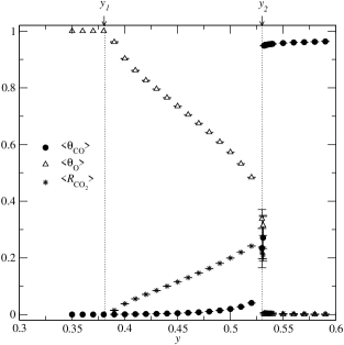
Figure 1: Average values of the CO and O coverages, $\theta_{\rm CO}$ and $\theta_{\rm O}$, and of the CO₂ production rate, $R_{\rm CO_{2}}$, shown as functions of the stationary applied CO pressure $y$, for $L=100$ with $k=0.02$. A continuous, nonequilibrium phase transition occurs at $y_{1}$, and a discontinuous one at $y_{2}(k)$.

One way to perturb the catalytic oxidation process in order to increase the CO₂ production is by switching the external pressure back and forth across the discontinuous transition $y_{2}(k)$ imbhil95 ; ehsasi89 ; vaporciyan88 ; cutlip83 ; hegedus80 . It has been shown that when the ZGB system without desorption is quickly oscillated between the low and high $\theta_{\text{CO}}$ phases by a periodic variation of the external pressure, there is considerable enhancement of the catalytic activity ziff86 ; lopez00 . The period and amplitude of the driving pressure must be calibrated very carefully in order to avoid driving the system irreversibly toward the CO poisoned state.

In other work machado04 we have calculated the lifetimes associated with the decay of the metastable states of the ZGB-k model. The system was prepared in the low (high) CO coverage phase with an initial pressure $y_{i}<y_{2}(k)$ ($y_{i}>y_{2}(k))$, and then $y$ was suddenly changed to $y_{f}>y_{2}(k)$ ($y_{f}<y_{2}(k)$). We then measured the time it took the system to leave the metastable state in both cases. We found that the lifetimes depend on the direction of the process, the decontamination time $\tau_{d}$ (from high to low CO coverage) being different from the poisoning time $\tau_{p}$ (from low to high CO coverage). Inspired by this result, we decided to subject the system to an oscillating pressure $y(t)$ that in a period $T=t_{d}+t_{p}$ takes the values ,

$$y=\left\{\begin{array}[]{ll}y_{l}&\mbox{during the time interval}\ t_{d}\\ y_{h}&\mbox{during the time interval}\ t_{p}\;,\end{array}\right.$$ (1)

located at both sides of the transition point, i.e., $y_{l}<y_{2}(k)<y_{h}$ (see Fig. 2(a)).

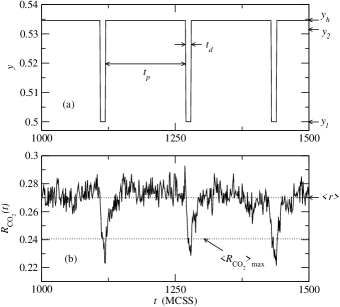
Figure 2: (a) Applied periodic pressure of CO, $y(t)$, that takes the values $y_{l}=0.5$ and $y_{h}=0.535$ during the time intervals $t_{d}=10$ and $t_{p}=150$, respectively. (b) Response of the production rate to the applied pressure given in (a) for $L=100$ with $k=0.02$. The dotted line marked $\langle r\rangle$ indicates the long-time average of the period-averaged CO₂ production rate $r$, defined by Eq. (2), while the dotted line marked $\langle R_{\rm CO_{2}}\rangle_{\rm max}$ marks the maximum average CO₂ production rate for constant $y=y_{2}(k)$, shown in Fig. 1. Time is measured in units of MCSS.

We found that, for each selection of $y_{l}$ and $y_{h}$, by tuning $t_{d}$ and $t_{p}$, the times that the driving force spends in the low and high coverage regions respectively, we could increase the productivity of the system. In Fig 2(b) it is seen that the response to the periodic pressure shown in Fig 2(a), the CO₂ production rate $R_{\text{CO}_{2}}$, also exhibits an oscillatory behavior. We therefore use its period-averaged value, defined as

$$r=\frac{1}{T}\oint R_{\text{CO}_{2}}(t)dt\;,$$ (2)

as the dynamic order parameter. For the parameters used in Fig. 2, the long-time average of $r$ is $\langle r\rangle=0.2683$, 11% higher than the maximum average CO₂ production rate for constant $y$, $\langle R_{\rm CO_{2}}\rangle_{\rm max}=0.2414$. (Compare Fig. 1 and Fig 2(b).)

By averaging $r$ over many periods of oscillation (of the order of $2\times 10^{3}$), we found that, depending on the values of $t_{d}$ and $t_{p}$, the system has two well-defined regimes: a productive one with $\langle r\rangle>0$, and a nonproductive one with $\langle r\rangle\approx 0$, separated by a transition line in the ($t_{p},t_{d}$) plane. Fig. 3 shows density plots of $\langle r\rangle$ in terms of $t_{d}$ and $t_{p}$ for two choices of $y_{l}$ and $y_{h}$.

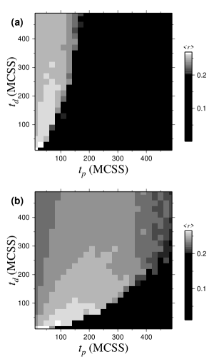
Figure 3: Long-time average $\langle r\rangle$ of the period-averaged CO₂ production rate $r$, shown as a density plot vs $t_{d}$ and $t_{p}$ for (a) $y_{l}=0.52$, $y_{h}=0.54$, and (b) $y_{l}=0.51$, $y_{h}=0.535$. $k=0.01$ and $L=100$.

The transition line depends strongly on the selected values of $y_{l}$ and $y_{h}$, as can be seen by comparing Fig. 3 (a) and Fig. 3 (b). This behavior can be understood by looking at the dependence of the lifetimes on the pressure. In Fig. 4 we show a schematic, but qualitatively correct, diagram of the lifetimes $\tau_{p}$ and $\tau_{d}$ vs $y$. The lifetimes increase rapidly as $y$ approaches the coexistence point $y_{2}(k)$, but the dependences of $\tau_{d}$ and $\tau_{p}$ on the distance to $y_{2}(k)$ are not equal (this is evident in the limiting case, $k\rightarrow 0$, where $\tau_{d}\rightarrow\infty$ independent of $y$), as the lifetimes depend on the direction of the decay. For the values of $y_{l}$ and $y_{h}$ selected in Fig. 4(a), the system takes longer to be decontaminated than to be poisoned, i.e., $\tau_{d}>\tau_{p}$, suggesting that the transition line (corresponding to the region of high CO₂ production) lies in the region $t_{d}>t_{p}$, as can be seen in Fig. 3 (a). When $y_{l}$ and $y_{h}$ are selected as in Fig. 4(b), the system takes less time to be decontaminated than to be poisoned, i.e., $\tau_{d}<\tau_{p}$. Then the transition line is expected to lie in the region $t_{d}<t_{p}$, as seen in Fig. 3 (b). The location of the transition line in each case is schematically indicated in Fig. 4(c).

Figure 4: (a) and (b): Schematic representations of the decay times of the metastable states as functions of the CO pressure $y$. The asymmetry of the curves indicates that the lifetimes depend on the direction of approach to the coexistence point, $y_{2}(k)$. The ratio $\tau_{d}/\tau_{p}$ depends on the values of $y_{l}$ and $y_{h}$, which are different in (a) and (b). (a) corresponds to the situation shown in Fig. 3 (a), and (b) corresponds to Fig. 3 (b). (c) Schematic representation of the dependence of the transition line between the phases with $\langle r\rangle>0$ and $\langle r\rangle\approx 0$, $t_{d}^{\ast}(t_{p})$, on how $y_{l}$ and $y_{h}$ are selected.

In Fig. 5 it can be seen how the average CO₂ production, $\langle r\rangle$, depends on $t_{d}$ for two different values of $t_{p}$ and $k$. When $k=0.01$, Fig. 5 (a) shows [consistent with Fig. 3 (a) and Fig. 3 (b)] that the system has two well-defined dynamic phases, one with $\langle r\rangle>0$ and the other with $\langle r\rangle\approx 0$. When $k$ is increased to 0.04, the system changes continuously from one phase to the other, as seen in Fig. 5 (b) and Fig. 6. This behavior suggests that for low values of $k$, the system has a dynamic phase transition (DPT) between a high CO₂ productive dynamic phase and a nonproductive one. This is reminiscent of the behavior of ferromagnetic Ising or anisotropic $XY$ or Heisenberg spin systems driven by a periodically oscillating field TOME90 ; MEND91 ; ACHAR97_1 ; ACHAR97_2 ; CHAK99 ; ising1 ; ising2 ; FUJI01 ; KORN02 ; JANG01 ; JANG03 ; YASU02 .

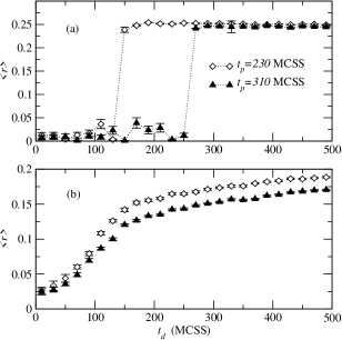
Figure 5: Long-time average of the period-averaged rate of CO₂ production, $\langle r\rangle$, shown vs $t_{d}$ for two values of $t_{p}$ and $L=100$; (a) with $y_{l}=0.52$, $y_{h}=0.535$, and $k=0.01$, and (b) with $y_{l}=0.52$, $y_{h}=0.553$, and $k=0.04$. Only for $k=0.01$ the system clearly presents two dynamic phases: one with $\langle r\rangle\approx 0$ and the other with $\langle r\rangle>0$.

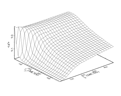
Figure 6: Surface plot of $\langle r\rangle$ vs $t_{d}$ and $t_{p}$ for $y_{l}=0.52$, $y_{h}=0.553$, and $k=0.04$. $L=100$.

Universality and finite-size scaling are well-known tools to analyze critical phenomena. Near a second-order equilibrium phase transition, the order-parameter correlation length diverges, leading to power-law singularities in terms of the finite system size $L$ pheno . Following the lead of previous applications to the DPT in the kinetic Ising model driven by an oscillating field ising1 ; ising2 , we use the period-averaged CO₂ production rate $r$ as a dynamic order parameter and perform a finite-size scaling analysis of its fluctuations and mean value. We define a measure of the fluctuations in $r$ in a $L\times L$ system in the standard way as

$$X_{L}=L^{2}[\langle r^{2}\rangle-\langle r\rangle^{2}]$$ (3)

and measure $X_{L}$ as a function of $t_{d}$ for a fixed value of $t_{p}$ and several values of $L$. Analogous to the situation at a second-order equilibrium phase transition, the order-parameter fluctuations increase with the system size, such that the maximum value of $X_{L}$ scales as $X_{L}^{\text{max}}\sim L^{\gamma/\nu}$, and the $n$th moment of the order parameter at the transition scales as $\langle r^{n}\rangle_{L}\sim L^{-n(\beta/\nu)}$. (We use standard notation for the critical exponents: $\gamma$ for the fluctuation exponent, $\beta$ for the order-parameter exponent, and $\nu$ for the correlation-length exponent GOLD92 .)

In Fig. 7 we show $X_{L}$ vs $t_{d}$ for four system sizes at $k=0.01$ and $k=0.04$. The errors in $X_{L}$ are obtained by standard error propagation analysis as $\sigma_{X_{L}}\approx 2X_{L}/\sqrt{n-1}$. Fig. 7 (a) shows that, for $k=0.01$ and the four values of $L$ used, $X_{L}$ displays a clear peak, which increases in height with increasing $L$. This is in clear contrast with Fig. 7 (b) for $k=0.04\approx k_{c}$, which shows no such increase with $L$.

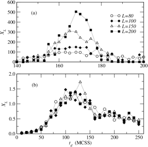
Figure 7: The order-parameter fluctuation measure $X_{L}$, shown vs $t_{d}$ for $t_{p}=230$, for four system sizes, (a) $k=0.01$ and (b) $k=0.04\approx k_{c}$. The dotted lines are guides to the eye. For clarity the error bars are not included in the plot. The highest values of $X_{L}$ have an error of approximately 6 %.

In Fig. 8(a) we plot $\ln(X_{L}^{\text{max}})$ versus $\ln(L)$ for $k=0.01$. A linear fit indicates a power-law divergence of the fluctuations with $L$, with exponent $\gamma/\nu=1.77\pm 0.02$. A different method to extract the power-law exponent, which has some advantage in eliminating the effects of a nonsingular background term (as in $X_{L}=f+gL^{\gamma/\nu}$ with $f$ and $g$ constants), is to consider

$$\ln\left[\frac{X_{bL}^{\text{max}}}{X_{L}^{\text{max}}}\right]/\ln b=\frac{\gamma}{\nu}+{\cal O}(1/\ln b)$$ (4)

with $L$ fixed at a relatively small value (here, $L=80$), and $b>1$. For large $L$ and $b$, the correction term is proportional to $f/(g\ln b)$, so that the exponent can be estimated by plotting the left-hand-side of Eq. (4) vs $1/\ln b$ and extrapolating to $1/\ln b=0$, as in Fig. 8(b). The resulting estimate is again $\gamma/\nu=1.77\pm 0.02$.

Figure 8: (a) Plot of $\ln(X_{L}^{\text{max}})$ vs $\ln(L)$ and (b) plot of $\ln(X_{bL}^{\text{max}}/X_{L}^{\text{max}})/\ln(b)$ vs $1/\ln(b)$, both for $k=0.01$ and $t_{p}=230$, and including all four system sizes. $X_{L}^{\text{max}}$ is the maximum value of $X_{L}$, taken from Fig. 7 (a). The straight lines are the best linear fits to the data and in both cases give $X_{L}^{\text{max}}\sim L^{\gamma/\nu}$ with $\gamma/\nu=1.77\pm 0.02$.

To obtain an estimate for the exponent ratio $\beta/\nu$, we used the scaling relation for the order parameter at the critical point, $\langle r^{n}\rangle\sim L^{-n(\beta/\nu)}$, (again with the possibility of a nonscaling background, which can be quite significant for $r$) to plot the left-hand side of

$$-\ln\left[\frac{\langle r^{n}\rangle_{bL}}{\langle r^{n}\rangle_{L}}\right]/\ln b=n\frac{\beta}{\nu}+{\cal O}(1/\ln b)$$ (5)

for $L=80$ vs $1/\ln b$, as shown in Fig. 9. For lack of a better estimate of the transition point, $\langle r^{n}\rangle$ were measured at the values of $t_{d}$ corresponding to the maxima of $X_{L}$. A linear fit that takes into account all four system sizes gives $\beta/\nu=0.14\pm 0.06$ for $n=2$ and $\beta/\nu=0.10\pm 0.03$ for $n=4$. As a combined estimate, we take $\beta/\nu=0.12\pm 0.04$, where the error bar includes some measure of our uncertainty about a nonscaling background and other finite-size effects.

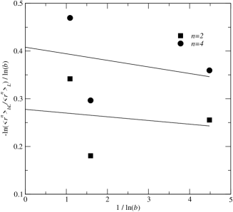
Figure 9: Plot of $-\ln(\langle r^{n}\rangle_{bL}/\langle r^{n}\rangle_{L})/\ln(b)$ vs $1/\ln(b)$ for $k=0.01$ and $t_{p}=230$, including all four system sizes. The straight lines are the best linear fits to the data, giving $\beta/\nu=0.14\pm 0.06$ for $n=2$ and $\beta/\nu=0.10\pm 0.03$ for $n=4$.

Combining the exponent estimates we find

$$2(\beta/\nu)+(\gamma/\nu)=2.01\pm 0.03\approx 2=d\;,$$ (6)

where $d$ is the spatial dimension. This result agrees with hyperscaling GOLD92 and indicates that our finite-size scaling results are internally consistent ENDNOTE . Results very similar to the ones presented above were obtained selecting the period-averaged CO coverage as the order parameter, instead of $r$.

Our estimated exponent ratios are very close to the analogous two-dimensional equilibrium Ising values ($\gamma/\nu=7/4=1.75$ and $\beta/\nu=1/8=0.125$ with $\beta=1$ GOLD92 ), but they are also near those for two-dimensional random percolation ($\gamma/\nu=43/24\approx 1.79$ and $\beta/\nu=5/48\approx 0.104$ with $\nu=4/3\approx 1.33$ STAU92 ). One way to verify the universality class without calculating $\nu$ directly (which would require much more accurate data than we have available), is to consider another universal quantity, such as the fixed-point value of the fourth-order order-parameter cumulant (“Binder cumulant”) pheno ,

$$u_{L}=1-\frac{\langle(r-\langle r\rangle_{L})^{4}\rangle_{L}}{3\langle(r-\langle r\rangle_{L})^{2}\rangle_{L}^{2}}\;,$$ (7)

where $\langle\bullet\rangle_{L}$ denotes the average over the whole time series of $r$ for an $L\times L$ system. This cumulant is shown vs $t_{d}$ for different $L$ in Fig. 10. The maximum possible value of $u_{L}$ is 2/3, which is reached in the dynamically ordered phase, provided that ergodicity is not broken or that $\langle r\rangle_{L}$ is exactly known. This is not so in the present case, and so the cumulant is nonmonotonic, becoming negative deep in both the dynamically ordered (large $t_{d}$) and disordered (small $t_{d}$) phases. With sufficiently accurate data, the curves representing $u_{L}$ for different $L$ cross or touch at a common point, which represents an estimate for the critical value of the control variable (here, $t_{d}$) that is quite insensitive to corrections to scaling. The value of $u_{L}$ at this fixed point, $u^{\ast}$, is a universal quantity characteristic of the particular universality class. In the present case, the accuracy of our data is not sufficient to use the crossing point as an estimate for the critical value of $t_{d}$ (we have instead used the maxima of $X_{L}$). However, $u^{\ast}$ is seen to be in the vicinity of 0.6, consistent with the very accurately known value for the two-dimensional Ising universality class, $u_{\rm Ising}^{\ast}=0.6106901(5)$ KAMI93 . Even though it is not very accurately determined, the value of $u^{\ast}$ observed for the present system is unlikely to be as low as the value for random percolation, $u_{\rm Perc}^{\ast}\approx 0.555$ ZIFFperc . Our total numerical finite-size scaling evidence thus points in the direction that the DPT in this system belongs to the two-dimensional equilibrium Ising universality class, together with other DPTs in far-from-equilibrium systems, such as the one observed in the two-dimensional kinetic Ising model driven by an oscillating applied field ising1 ; ising2 ; FUJI01 ; ENDNOTE2 .

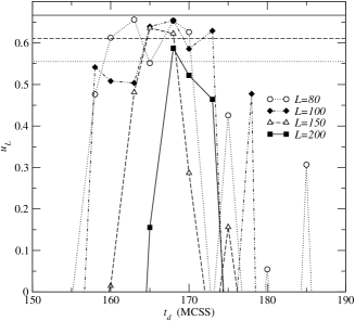
Figure 10: The fourth-order cumulant $u_{L}$, shown vs $t_{d}$ for all four system sizes, $k=0.01$ and $t_{p}=230$. The horizontal lines correspond to $u_{L}=2/3$ (solid), $u_{\rm Ising}^{\ast}\approx 0.610$ (dashed), and $u_{\rm Perc}^{\ast}\approx 0.555$ (dotted). See discussion in the text. The errors are approximated by standard error-propagation methods and are of the order of 3 % for the highest values of $u_{L}$ and of the order of 14 % for the lowest.

An independent indication that the DPT in this system belongs to the equilibrium Ising universality class, is a symmetry argument due to Grinstein, Jayaprakash, and He GRIN85 , who argued that the equilibrium Ising universality class extends to nonequilibrium cellular automata that (i) have local dynamics, (ii) do not conserve the order parameter or other auxiliary fields, and (iii) respect the Ising up-down symmetry. This result was later extended by Bassler and Schmittmann BASS94 , using renormalization-group arguments, to systems that obey conditions (i) and (ii) above, but violate (iii), such as some driven lattice gases. The ZGB-k model satisfies these requirements, and it should thus belong to the equilibrium Ising class on symmetry grounds.

IV Conclusions

In this paper we have studied the dynamic response of the ZGB model with CO desorption (the ZGB-k model tome93 ) to periodic variations of the relative CO pressure $y$, around the coexistence value $y_{2}(k)$ that separates the low and high CO-coverage phases. There is an asymmetry of the lifetimes of the model: its decontaminating time $\tau_{d}$ generally differs from the contaminating time $\tau_{p}$. We exploited this fact by selecting a square-wave periodic CO pressure that stays for a time $t_{d}$ in the high-production region and for a time $t_{p}$ in the low-production one. We found that $t_{d}$ and $t_{p}$ can be tuned to significantly enhance the time-averaged catalytic activity of the system beyond its maximum value under constant-pressure conditions – a result we believe should be of applied significance.

We also found strong indications that, for sufficiently low values of the desorption rate, this driven nonequilibrium system undergoes a dynamic phase transition between a dynamic phase of high CO₂ production, $\langle r\rangle>0$, and a nonproductive phase $\langle r\rangle\approx 0$. As the order parameter for this nonequilibrium phase transition we used the period-averaged rate of CO₂ production, $r$. Our study shows that the distinction between these phases disappears for a high enough desorption rate. Applying finite-size scaling techniques in a similar fashion to what is commonly done to study equilibrium second-order phase transitions, we found that, for small values of the CO desorption rate $k$, the fluctuations of the order parameter diverge as a power law with the system size, $X_{L}^{\text{max}}\sim L^{\gamma/\nu}$ with exponent $\gamma/\nu=1.77\pm 0.02$, while moments of the order parameter at the transition point decay as $\langle r^{n}\rangle_{L}\sim L^{-n\beta/\nu}$ with $\beta/\nu=0.12\pm 0.04$, and the fourth-order order-parameter cumulant $u_{L}$ has a fixed-point value of $u^{\ast}\approx 0.6$. These values are close to those of the two-dimensional Ising universality class, and together with general symmetry arguments GRIN85 ; BASS94 they represent reasonable evidence that this far-from equilibrium phase transition belongs to the same universality class as the equilibrium Ising model. A a higher level of confidence about the universality class would require simulations at least an order of magnitude more extensive than the ones presented here – a task beyond the scope of the present paper.

Finally, we note that the enhancement of the CO₂ production and the continuous DPT are probably closely related phenomena since the critical cluster associated with the phase transition is likely to provide more empty sites available for O₂ adsorption near adsorbed CO molecules, than the sharp interfaces expected near the first-order coexistence line seen under constant-$y$ conditions.

- (1) H. J. Jensen, Self-Organized Criticality: Emergent Complex Behavior in Physical and Biological Systems (Cambridge University Press, Cambridge, England, 1998).
- (2) J. Marro and R. Dickman, Nonequilibrium Phase Transitions in Lattice Models (Cambridge University Press, Cambridge, England, 1999).
- (3) K. Christmann, Introduction to Surface Physical Chemistry (Steinkopff Verlag, Darmstadt 1991); V. P. Z. Zhdanov and B. Kazemo, Surf. Sci. Rep. 20, 111 (1994).
- (4) G. C. Bond, Catalysis: Principles and Applications (Clarendon, Oxford, 1987).
- (5) R. Imbhil and G. Ertl, Chem. Rev. 95, 697 (1995).
- (6) M. Ehsasi, M. Matloch, O. Frank, J. H. Block, K. Christmann, F. S. Rys and W. Hirschwald, J. Chem. Phys. 91, 4949 (1989).
- (7) G. Vaporciyan, A. Annapragada, and E. Gulari, Chem. Eng. Sci. 43, 2957 (1988).
- (8) M. B. Cutlip, C. J. Hawkins, D. Mukesh, W. Morton, and C. N. Kenney, Chem. Eng. Commun. 22, 329 (1983).
- (9) L. L. Hegedus, C. C. Chang, D. J. McEwen, and E. M. Sloan, Ind. Eng. Chem. Fundam. 19, 367 (1980).
- (10) T. Matsushima, H. Hashimoto and I. Toyoshima, J. Catal. 58, 303 (1979).
- (11) A. Golchet and J. M. White, J. Catal. 53, 266 (1978).
- (12) K. Christmann and G. Ertl, Z. Naturforsch. Teil A 28, 1144 (1973).
- (13) R. M. Ziff, E. Gulari, and Y. Barshad, Phys. Rev. Lett. 56, 2553 (1986).
- (14) A. C. López and E. V. Albano, J. Chem. Phys. 112, 3890 (2000).
- (15) M. Tammaro and J. W. Evans, J. Chem. Phys. 108, 762 (1998).
- (16) T. Tomé and R. Dickman, Phys. Rev. E 47, 948 (1993).
- (17) E. Machado, G. M. Buendía, and P. A. Rikvold, in preparation.
- (18) T. Tomé and M. J. de Oliveira, Phys. Rev. A 41, 4251 (1990).
- (19) J. F. F. Mendes and J. S. Lage, J. Stat. Phys. 64, 653 (1991).
- (20) M. Acharyya, Phys. Rev. E 56, 1234 (1997).
- (21) M. Acharyya, Phys. Rev. E 56, 2407 (1997).
- (22) B. Chakrabarti and M. Acharyya, Rev. Mod. Phys. 71, 847 (1999).
- (23) S. W. Sides, P. A. Rikvold and M. A. Novotny, Phys. Rev. Lett. 81, 834 (1998); Phys. Rev. E 59, 2710 (1999).
- (24) G. Korniss, C. J. White, P. A. Rikvold and M. A. Novotny, Phys. Rev. E 63, 016120 (2000).
- (25) H. Fujisaka, H. Tutu, and P. A. Rikvold, Phys. Rev. E 63, 016120 (2001); Erratum: 63 059903(E) (2001).
- (26) G. Korniss, P. A. Rikvold, and M. A. Novotny, Phys. Rev. E 66, 056127 (2002).
- (27) H. Jang and J. Grimson, Phys. Rev. E 63, 066119 (2001).
- (28) H. Jang, J. Grimson, and C. K. Hall, Phys. Rev. B 67, 094411 (2003); 68, 046115 (2003).
- (29) T. Yasui, H. Tutu, M. Yamamoto, and H. Fujisaka, Phys. Rev. E 66, 036123 (2002); Erratum: 67, 019901(E) (2003).
- (30) K. Binder, in Finite Size Scaling and Numerical Simulation of Statistical Systems, edited by V. Privman (World Scientific, Singapore, 1990).
- (31) See, e.g., N. Goldenfeld, Lectures on Phase Transitions and the Renormalization Group (Addison-Wesley, Reading, MA, 1992).
- (32) We also tried to perform fits to determine the exponent ratios, excluding the results for the smallest system size, . We did this by using Eqs. (4) and (5) with . The resulting exponent estimates, , for , and for , are strongly -dependent and significantly violate the hyperscaling relation: for and for . These fits are thus not internally consistent, probably because the uncertainty in our data is such that the maximum range of system sizes is required to obtain reasonably accurate exponent ratios.
- (33) D. Stauffer and A. Aharony, Introduction to Percolation Theory, 2nd Ed. (Taylor & Francis, London, 1992).
- (34) G. Kamieniarz and H. W. J. Blöte, J. Phys. A: Math. Gen. 26, 201 (1993).
- (35) We were unable to find the fixed-point value of the fourth-order cumulant for random percolation in the literature, and we therefore calculated it ourselves by Monte Carlo simulation. Specifically, we used bond percolation on an square lattice with a square boundary and used as the order parameter the probability that a randomly chosen bond belongs to the percolating cluster. For and 200, the cumulants touch at the exactly known critical , giving .
- (36) The similarity with the Ising model with its “up-down symmetry” is most easily seen by defining the effective “magnetization” variable as in the standard Ising/lattice gas mapping.
- (37) G. Grinstein, C. Jayaprakash, and Y. He, Phys. Rev. Lett. 55, 2527 (1985).
- (38) K. E. Bassler and B. Schmittmann, Phys. Rev. Lett. 73, 3343 (1994).