Simulations of lattice animals and trees

Abstract

The scaling behaviour of randomly branched polymers in a good solvent is studied in two to nine dimensions, using as microscopic models lattice animals and lattice trees on simple hypercubic lattices. As a stochastic sampling method we use a biased sequential sampling algorithm with re-sampling, similar to the pruned-enriched Rosenbluth method (PERM) used extensively for linear polymers. Essentially we start simulating percolation clusters (either site or bond), re-weigh them according to the animal (tree) ensemble, and prune or branch the further growth according to a heuristic fitness function. In contrast to previous applications of PERM, this fitness function is not the weight with which the actual configuration would contribute to the partition sum, but is closely related to it. We obtain high statistics of animals with up to several thousand sites in all dimension $2\leq d\leq 9$. In addition to the partition sum (number of different animals) we estimate gyration radii and numbers of perimeter sites. In all dimensions we verify the Parisi-Sourlas prediction, and we verify all exactly known critical exponents in dimensions 2, 3, 4, and $\geq 8$. In addition, we present the hitherto most precise estimates for growth constants in $d\geq 3$. For clusters with one site attached to an attractive surface, we verify for $d\geq 3$ the superuniversality of the cross-over exponent $\phi$ at the adsorption transition predicted by Janssen and Lyssy, but not for $d=2$. There, we find $\phi=0.480(4)$ instead of the conjectured $\phi=1/2$. Finally, we discuss the collapse of animals and trees, arguing that our present version of the algorithm is also efficient for some of the models studied in this context, but showing that it is not very efficient for the ‘classical’ model for collapsing animals.

I Introduction

Lattice animals (or polyominoes, as they are sometimes called in mathematics Golomb ) are just clusters of connected sites on a regular lattice. Such clusters play an important role in many models of statistical physics, as e.g. percolation Stauffer92 , the Ising model (Fortuin-Kastleyn clusters, Swendsen-Wang algorithm Fortuin ; Swendsen ), and even lattice gauge theories Drouffe . The basic combinatorial problem associated to them is to count the number $Z_{N}$ of different animals of $N$ sites. Two animals are considered as identical, if they differ just by a translation (i.e., we deal with fixed animals in the notation of Jensen03 ), but are considered as different, if a rotation or reflection is needed to make them coincide. Thus there are e.g. $d$ animals of $N=2$ sites on a simple hypercubic lattice of dimension $d$, and $d(2d-1)$ animals with $N=3$.

The animal problem can be turned into a statistical problem by giving a statistical weight to every cluster. In contrast to percolation, where different shapes acquire different weights, all clusters with the same number $N$ of sites are given the same weight. This is similar to self avoiding walks (SAW). A SAW on a lattice is a connected cluster of $N$ sites with equal weight on all clusters, but with a restriction on its shape: each SAW has to be topologically linear, i.e. each site is connected by bonds to at most 2 neighbours. No such constraint holds for animals, thus animals are the natural model for randomly branched polymers Lubensky .

In addition to animals (or site animals, to be more precise) one can also consider bond animals and lattice trees. A bond animal is a cluster where bonds can be established between neighbouring sites (just as in SAWs), and connectivity is defined via these bonds: if there is no path between any two sites consisting entirely of established bonds, these sites are considered as not connected, even if they are nearest neighbours. Different configurations of bonds are considered as different clusters, and clusters with the same number of bonds (irrespective of their number of sites) have the same weight Rensburg97 . Weakly embeddable trees are bond animals with tree topology, i.e. the set of weakly embeddable trees is a subset of bond animals, each with the same statistical weight. Strongly embeddable trees are, in contrast, the subset of site animals with tree-like structure. All these definitions are illustrated in Fig. 1.

Figure 1: (a): A site animal with 8 sites; (b) A site tree (“strongly embeddable tree”); (c) A bond animal which is not a tree; (d) A bond tree (“weakly embeddable tree”).

Like many other statistical models, animals are characterized by scaling laws in the limit of large $N$. It is believed that all the above statistics (site and bond animals, weakly and strongly embeddable trees) are in the same universality class (same exponents, same scaling functions) which is that of randomly branched polymers. The number of animals (i.e. the microcanonical partition sum) should scale as Lubensky

$$Z_{N}\sim\mu^{N}N^{-\theta}\;,$$ (1)

and the gyration radius as

$$R_{N}\sim N^{\nu}\;,$$ (2)

Here $\mu$ is the growth constant or inverse critical fugacity, and is not universal. In contrast, the Flory exponent $\nu$ and the entropic exponent $\theta$ should be universal.

In spite of the obvious similarity to the SAW and percolation problems, there are a number of features in which the animal problem is unusual:

• The upper critical dimension is $d=8$. There, $\nu=1/4$ and $\theta=5/2$ Adler .

• The model is not conformally invariant Miller93 , and thus the Flory exponent $\nu$ is not known exactly in $d=2$.

• Using supersymmetry, it has been argued by Parisi and Sourlas  Parisi that the animal problem in $d$ dimensions is related to the Yang-Lee problem (Ising model in an imaginary external field) in $D=d-2$ dimensions. Based on this relationship (which is now proven rigorously Imbrie , using a mapping onto the hypercubes problem at negative fugacity Baxter ) they argued that $\theta$ and $\nu$ should not be independent, but

  $$\theta=(d-2)\nu+1\;.$$ (3)

  This implies in particular that $\theta=1$ in $d=2$. In addition, they showed that $\nu=1/2$ in $d=3$.

• Assuming universality so that scaling of the hard squares model at negative fugacity can be inferred from Baxter’s solution of the hard hexagon model, and mapping the hard squares model onto lattice animals in 4 dimensions, Dhar Dhar obtained $\theta=11/6$ for $d=4$. Thus one knows the exact values of $\nu$ for $d=1,3,4$, and 8, but not for $d=2,5,6$, and 7.

• In a series of papers, Janssen and Lyssy Janssen92 ; Janssen94 ; Janssen95 studied animals attached to an adsorbing plane surface. For weak adsorption (high temperature) the animals have basically the same structure as in the bulk, and the partition sum has the same scaling, $Z^{\prime}_{N}\sim\mu^{\prime N}N^{-\theta^{\prime}}$ with $\mu^{\prime}=\mu$ and $\theta^{\prime}=\theta$ DeBell ; DeBell92 ; footnoteDeBell . For strong adsorption (low temperature) there is an adsorbed phase. Janssen and Lyssy argued that the cross-over exponent between these two phases should be super-universal, $\phi=1/2$ for all dimensions $d\geq 2$.

In the present paper we address all these points by means of a novel Monte Carlo algorithm which follows essentially the strategy used in the pruned-enriched Rosenbluth method (PERM) g97 . This is a recursively (depth first) implemented sequential sampling method with importance sampling (bias) and re-sampling (“population control”). It seems that PERM in the present implementation is much more efficient than previous sampling methods for animals and trees. Indeed we shall present numerous new estimates for critical exponents and growth constants which had previously been measured only with much larger error bars or not at all.

All this holds for athermal animals and trees, i.e. when there are no attractive forces between monomers. When such forces become strong, a number of different collapse phase transitions are claimed to occur, depending on the detail of the model Derrida-H ; Dickman ; Lam87 ; Lam88 ; Madras90 ; Flesia92 ; Flesia94 ; Seno94 ; Henkel96 ; Stratychuk95 ; Madras97 ; Rensburg99 ; Rensburg00 . The simplest one of these involves site animals and a simple contact energy for each occupied nearest neighbour pair Derrida-H ; Dickman ; Lam87 ; Lam88 and is undisputed. But another transition, between two collapsed phases with different densities of bonds Madras90 ; Flesia92 ; Flesia94 ; Madras97 ; Rensburg00 , is still controversial Seno94 ; Henkel96 ; Stratychuk95 . At present all versions of our algorithm become inefficient for the first model, when the collapse point is approached. This is a bit disappointing in view of the fact that PERM for linear polymers is dramatically more efficient at the coil-globule transition than for athermal SAWs g97 . Obviously this leaves much room for further improvements. On the other hand, our method should work well for the other transition in large parts of the phase diagram.

Details of the algorithm for site animals will be given in Sec. 2. Detailed studies of site animals in the bulk and in contact with a wall will be presented in Secs. 3 and 4. Bond animals and trees will be discussed in Sec. 5. Finally, in Sec. 6 we will study animal (and tree) collapse due to attractive forces between monomers. The paper ends with conclusions in Sec. 7.

II Numerical Methods

II.1 Previous Methods

II.1.1 $\epsilon$-Expansions

Field theoretic $\epsilon$-expansions (where $\epsilon$ is the distance from the critical dimension) were applied already very early to animals Lubensky and to the Yang-Lee problem Alcantara . When the relationship between both problems was established, the latter gave the most precise predictions for critical animal behaviour in high dimensions ($d\geq 5$).

II.1.2 Exact Enumeration

Exact enumeration of animals and trees is surprisingly non-trivial Martin ; Redner79 ; Redelmeier ; Mertens . Nevertheless, very extensive enumerations have recently been performed by I. Jensen Jensen00 ; Jensen01 ; Jensen03 for site animals and site trees in $d=2$. At present they give the best numerical verification of the prediction $\theta=1$, and they give the most precise estimates for the Flory exponent ($\nu=0.64115\pm 0.00005$) and for the growth constants: $\mu=4.0625696\pm 0.0000005$ for animals Jensen03 , and $3.795254\pm 0.000008$ for trees. These values are more precise than old estimates obtained by finite size scaling using strip geometry Derrida-S . There are also enumerations of various animals and trees in higher dimensions Peters ; Sykes ; Gaunt82 ; Whittington ; Lam ; Adler ; Madras90 ; Edwards ; Foster , but they are much less complete and in general they do not at present give the best estimates for critical parameters.

II.1.3 Markov Chain Monte Carlo Methods

The latter are obtained nowadays by Markov chain Monte Carlo (MCMC) methods. Such algorithms have been used for animals since at least 20 years Stauffer ; Seitz ; Dickman ; Glaus . At present, the most efficient MCMC algorithm for lattice trees is a version of the pivot algorithm Rensburg92 ; Rensburg97 ; You98 ; You01 ; Rensburg03 . These simulations showed that $\nu=1/2$ in $d=3$, as predicted by Parisi . Simulations of animals attached to an attractive wall verified that indeed $\phi=1/2$ in $d=2$ You01 (as also verified with transfer matrix and similar methods Queiroz ; Vujic ), although simulations in $d=3$ gave $\phi\approx 0.714$ Lam-Binder , in gross violation of the Janssen-Lyssy prediction.

When applied to SAWs, the pivot algorithm works by choosing a pivot point and proposing a rotation of the shorter arm around the pivot, and accepting it when this leads to no violation of self avoidance Madras . When adapted to trees, one again chooses a random pivot point, but now the entire branch hinging on this pivot is cut and glued somewhere else. Again this move is accepted only if this leads to no violation of self avoidance and if it would not lead to wrong cluster topology.

This method also allows to estimate growth constants, if it is used together with the atmosphere method Rensburg03 . In the latter, it is counted how many possible ways there exist to grow the cluster by one further step, giving in this way an estimate of $Z_{N+1}/Z_{N}$. Basically the same method had been used in Grassberger03 to obtain very precise estimates for the critical percolation thresholds in high dimensional lattices.

II.1.4 Cluster Growth (‘Sequential Sampling’, ‘Static’) Methods

The first stochastic growth algorithm for trees seems to have been devised by Redner Redner . Similar methods were then used by Meirovitch Meirovitch and Lam Lam for animals. But already Leath seems to have realized that his well known algorithm for growing percolation clusters Leath could be used also for the study of animals, simply by reweighing the clusters. Recently this was taken up systematically in Care .

In the following we shall discuss the latter in some detail, and we shall restrict our discussion to site animals. The authors of Care basically use a standard growth algorithm for percolation clusters Leath ; Grassberger83 ; Swendsen2 , and then reweigh the cluster so that they obtain the correct weight for the animal ensemble. In a percolation cluster growth algorithm for site percolation, one starts with a single seed site and writes it into an otherwise empty list of ‘growth sites’. Then one recursively picks one item in the list of growth sites, removes it from the list and adds it with probability $p$ to the cluster, and adds all its wettable neighbours to the list. This is repeated until either the cluster size exceeds some fixed limit (in which case the cluster is discarded), or until the list is empty. A cluster with $N$ sites, $b$ boundary sites, and with fixed shape is obviously obtained with probability

$$P_{Nb}=p^{N}(1-p)^{b},$$ (4)

i.e. with the correct probability so that any unweighed average is just an average over the percolation ensemble. Repeating this many times, the animal partition sum is then

$$Z_{N}=\langle 1/P_{Nb}\rangle=p^{-N}\langle(1-p)^{-b}\rangle\;.$$ (5)

The authors of Care called their method a Rosenbluth method, in view of the obvious analogy with the Rosenbluth-Rosenbluth method Rosenbluth55 for SAWs. In the latter one also samples from a biased ensemble and then reweighs each configuration with the inverse of the sampling probability to obtain the correct partition sum.

II.2 PERM

Like the original Rosenbluth-Rosenbluth method for SAWs, the method of Care has the disadvantage that the weights have a very wide distribution for large $N$. Thus even a very large sample will finally, when $N$ gets too big, be dominated by a single configuration, and the method becomes inefficient even though it is easy to generate huge samples.

PERM (or any other strategy with resampling) tries to avoid this by trimming the width of the distribution of weights, by pruning configurations with very low weight and making clones of high weight configurations which then share the weight among themselves. In many situations this has proven to be extremely efficient permreview ; star1 ; star2 . But we cannot yet apply it to animals, since we have to be able to estimate the weight of a cluster while it is still growing, and up to now we have only discussed the relationship between animals and percolation clusters after they had stopped growing.

In the following we shall again discuss only site animals, bond animals and trees being discussed in Sec. 5.

To obtain the relationship between still growing percolation clusters and animals, let us consider a cluster with $N$ sites, $g$ growth sites, and $b$ sites which definitely belong to the boundary. At each of the growth sites the cluster can grow further, or it can stop growing with probability $1-p$. Thus this cluster will contribute with weight $(1-p)^{g}$ to the sample of percolation clusters with $N$ sites and $b+g$ boundary sites. Its contribution to the animal ensemble is smaller by a factor $[p^{N}(1-p)^{b+g}]^{-1}$, and we have thus

$$Z_{N}=p^{-N}\langle(1-p)^{-b}\rangle\;.$$ (6)

This is exactly the same formula as above, but now the average is taken over all growing clusters, while before we had averaged over clusters which had stopped growing.

Before we can implement these ideas, we have to discuss two problems:
(a) How are the clusters to be grown precisely?
(b) On what basis should we decide when to prune and when to clone a cluster?
As we shall see, both questions are not trivial.

Figure 2: Growing clusters generated breadth first (top) and depth first (bottom). In both cases we used $p=p_{c}=0.5927$, and in both cases $N=4000$. Occupied sites are depicted by small points, growth sites by heavy dots. Both figures are plotted with the same scale.

(a) Percolation cluster growth algorithms can be depth first or breadth first. In the former, growth sites are written into a first-in last-out list (a stack). A typical code for this is given in Swendsen2 . For a breadth first implementation we use, instead, a first-in first-out list (‘fifo-list’ or queue). Two 2-$d$ clusters growing according to these two schemes, with $p=p_{c}=0.5927$, are shown in Fig. 2. Both have $N=4000$. But the cluster grown using a stack has a completely different shape and has $\approx 3$ times as many growth sites as the one grown with a queue! Most of these growth sites are nearly dead (their descendents will die after a few generations), but this is not realized because they are never tested. Since also the fluctuations in the number of growth sites are much bigger in a depth first implementation, the weights in Eq.(6) will also fluctuate much more, and we expect much worse behaviour. This is indeed what we found numerically: Results obtained when using a stack for the growth sites were dramatically much worse than results obtained with a queue.

Notice that this is independent of the way how pruning and cloning is done. Indeed we implemented this “population control” recursively as a depth first strategy, as was done for all previous applications of PERM.

In addition, there are also some minor ambiguities in percolation cluster growth algorithms, such as the order in which one searches the neighbours of a growth site and writes them into the list. In 2 dimensions one can e.g. use the preferences east-south-west-north, or east-west-north-south, or a different random sequence at every point. We found no big differences in efficiency.

(b) In most previous applications of PERM, the best strategy was to base the decision whether to prune or branch directly on the weight with which the configuration contributes to the partition sum footnote0 . This would mean in the present case that we clone, if $W_{n}\equiv p^{-n}(1-p)^{-b}>c_{+}\hat{Z_{n}}$ where $c_{+}$ is a constant of the order $1\ldots 10$ and $\hat{Z_{n}}$ is the current estimate of $Z_{n}$. Similarly, a cluster would be killed (with probability 1/2 g97 ), if $W_{n}<c_{-}\hat{Z_{n}}$ with $c_{-}$ slightly smaller than 1.

In the present case this would not be optimal, since it would mean that mostly clusters with few growth sites are preferred (they tend to have larger values of $b$, for the same $n$), and these clusters would die soon and would contribute little to the growth of much larger clusters. Thus we defined a fitness function

$$f_{n}=W_{n}/(1-p)^{\alpha g}=p^{-n}(1-p)^{-b-\alpha g}$$ (7)

with a parameter $\alpha$ to be determined empirically, and used

$$f_{n}>c_{+}\langle f_{n}\rangle,\qquad f_{n}<c_{-}\langle f_{n}\rangle$$ (8)

as criteria for cloning and pruning. We checked in quite extensive simulations that best results were obtained with $\alpha=1$ (except when $N$ is small), and in the following we shall use only this choice.

Finally we have to discuss the optimal values of $p$. It is clear that we should not use $p>p_{c}$, where $p_{c}$ is the critical percolation threshold. Since minimal reweighing is needed for small $p$ (subcritical percolation is in the animal universality class), one might expect $p\ll p_{c}$ to be optimal. This is indeed true for small values of $N$ (which we are not primarily interested in), but not for large $N$. For the latter it is more important that clusters grown with $p\ll p_{c}$ have to be cloned excessively, since they otherwise would die rapidly in view of their few growth sites.

To decide this problem empirically, we show in Fig. 3 the errors of the estimated free energies $F_{N}=-\ln Z_{N}$ for $d=2$. More precisely, we show there one standard deviation multiplied by the square root of the CPU time (measured in seconds), for different values of $p$. Each simulation was done on a Pentium with 3 GHz using the gcc compiler under Linux, and each simulation was done for $N_{\rm max}=4000$ (although we plotted some curves only up to smaller $N$, omitting data which might not have been converged). We see clearly that small values of $p$ are good only for small $N$. As $N$ increases, the best results were obtained for $p\to p_{c}$. The same behaviour was observed also in all other dimensions, and also for animals on the bcc and fcc lattices in 3 dimensions (data not shown). As an example we show in Fig. 4 the analogous results for $d=8$. There we used a 64 bit machine (a 600 MHz Compaq ALPHA), because this simplified hashing (for large $d$ we used hashing as described e.g. in Grassberger03 ).

Notice that the errors shown in Fig. 4 are much smaller than those in Fig. 3, although the machine was slower and the animals were twice as large ($N_{\rm max}=8000$). Indeed, the errors decreased monotonically with $d$, being largest for $d=2$. Using $p$ slightly smaller than $p_{c}$ we can obtain easily very high statistics samples of animals with several thousand sites for dimensions $\geq 2$. A typical 2-$d$ animal with 12000 sites is shown in Fig. 5, and a 3-$d$ animal on the bcc lattice with 16000 sites is shown in Fig. 6.

Figure 3: Statistical errors of $\ln Z$ for lattice animals in $d=2$ for various values of $p$. To make the different runs comparable, errors are multiplied by the square root of the CPU time measured in seconds. In 2 dimensions $p_{c}=0.5927$.

Figure 4: Same as Fig. 3, but for $d=8$ where $p_{c}=0.0752$. The straightest curve corresponds to the largest $p$.

Figure 5: A typical lattice animal with $12000$ sites on the square lattice.

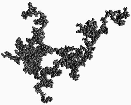
Figure 6: A 3-$d$ lattice animal with $16000$ sites on the bcc lattice.

Figure 7: Log-log plot of distributions of tour weights of $2d$ animals with $N=4000$, for $p=0.57$ and for $p=0.47$, together with a straight line representing the function $y=const/W$.

To check the reliability of our error bars we looked at distributions of tour weights as described in Grass99 . A tour is the set of all configurations generated by cloning from one common start and therefore possibly being strongly correlated. If the distribution $P$ of tour weights $W$ is very broad, we are back to the problem of the Rosenbluth method that averages might be dominated by a single tour. To check for this, we plot $P(\ln W)$ against $\ln W$, and compare its right hand tail to the function $1/W$. If the tail decays much faster, we are presumably on the safe side, because then the product $WP(\ln W)$ has its maximum where the distribution is well sampled. If not, then the results can still be correct, but we have no guarantee for it.

In Fig. 7, we show these tour weight distributions for two-dimensional animals with 4000 sites, for $p=0.57$ and for $p=0.47$ footnote1 . We see that the simulation with $p=0.57$ is on the safe side, but not that for $p=0.47$. Similar plots for other simulations described in this paper showed that all results reported below are converged and reliable.

Error bars quoted in the following on raw data (partition sums, gyration radii, and average numbers of perimeter sites or bonds) are straightforwardy obtained single standard deviations. Their estimate is easy since clusters generated in different tours are independent, and therefore errors can be obtained from the fluctuations of the contributions of entire tours (notice that clusters within one tour are not independent, and estimating errors from their individual values would be wrong).

On the other hand, errors on critical exponents and on growth constants are obtained by extrapolation. This is an ill-posed problem, and therefore any error obtained this way is to some degree subjective. All such errors quoted in the following are based on plotting the data in different ways, plotting effective exponents against different powers of $1/N$, trying different ansatzes for higher order correction to scaling terms, etc. They are not based on simply making least square fits over fixed intervals of $N$, as this could lead to very large underestimations of corrections to scaling. All quoted numbers are such that we believe, to the best of our knowledge, that the true value is most likely within one quoted error bar.

The total CPU time spent on the simulations reported in this paper is $\approx 25,000$ hours on fast PCs and work stations.

III Site Animals in 2 to 9 Dimensions

III.1 $d=2$

Figure 8: Deviations of the logarithm of the number of 2-$d$ site animals from exact enumerations of I. Jensen Jensen01 .

Figure 9: Relative deviations of the squared radii of gyration from exact values of Jensen01 .

Before we report our final results, we show one more test where we compare our raw data for $d=2$ with the exact enumerations of Jensen03 . In Fig. 8 we show the true relative errors of our estimates of the partition sum. Although there is some systematic trend visible, this is still within two standard deviations and thus not significant (notice that our values for different $N$ are not independent). Relative errors of the squared gyration radii are shown in Fig. 9. These data show that our estimates are basically correct, including the error bars.

Figure 10: Plot of $\ln Z_{N}-aN+\theta\ln N$ against $\ln N$ for $d=2$, with $a=1.401812,1.4018155$, and 1.401819 (top to bottom). Error bars are plotted only for the central curve.

Figure 11: Plot of $R_{N}^{2}/N^{2\nu}$ against $\ln N$ for $\nu=0.6406,0.6412$, and 0.6418. Again, error bars are plotted only for the central curve.

Plotting directly our values of $Z_{N}$ would not be very informative, neither would be a plot of $\ln Z_{N}-aN$, where $a=\ln\mu$. Both ways of plotting would hide any statistical errors. A more meaningful way of plotting our full data for $Z_{N}$ is used in Fig. 10, where we plot $\ln Z_{N}-aN+\ln N$ against $N$ for three values of $a$. Error bars are shown only for the central curve, although all three curves have of course the same errors. In view of Eq. (1), and accepting the prediction that $\theta=1$, we would expect a curve which becomes horizontal for large $N$. This is indeed seen for the central curve, but the obvious corrections to scaling make a precise estimate of $\mu$ difficult. The same is true for the gyration radii. In Fig. 11 we show $R_{N}^{2}/N^{2\nu}$ against $N$ for three candidate values of $\nu$. Again strong corrections to scaling are seen.

Figure 12: Same data as in Fig. 10, but plotted against $1/N^{0.9}$.

Figure 13: Same data as in Fig. 11, but plotted against $1/N^{0.9}$.

For these corrections one expects

$$Z_{N}\sim\mu^{N}N^{-\theta}(1+b_{Z}N^{-\Delta}+\cdots)$$ (9)

and

$$R^{2}_{N}\sim N^{2\nu}(1+b_{R}N^{-\Delta}+\cdots)\;,$$ (10)

where $\Delta$ is the correction exponent Adler , $b_{Z}$ and $b_{R}$ are non-universal amplitudes, and the dots stand for higher order terms in $1/N$. Notice that $\Delta$ is universal, and is the same in both equations. There are several methods discussed in the literature for estimating $\Delta$. We estimated it by plotting $\ln Z_{N}-aN+\ln N$ and $R^{2}_{N}/N^{2\nu}$ against $x\equiv 1/N^{\delta}$. Straight lines are expected near $x=0$ if and only if $\delta=\Delta$. We could not find a value of $\delta$ where these lines were absolutely straight for all $x$, but the straightest behaviour near $x\approx 0$ was obtained with $\delta\approx 0.9$, see Figs. 12 and 13.

Table 1: Main results for site animals. For convenience we also give in the second column the critical $p$-values for site percolation.

$d$	$p_{c}$	$a=\ln\mu$	$\theta$	$\nu$	$\frac{\theta}{(d-2)\nu+1}$	$\Delta$	Method
2	0.5927	1.4018155(30)	1a),c)	0.6412(5)	–	0.9(1)	present work
		1.401815696(5)		0.64115(5)	–	1.0	Series Jensen03 ; Jensen00
				0.642(10)	–	0.65(20)	MC You98
3	0.3116	2.1218588(25)	3/2a),c)	1/2a),c)	1a),c)	0.75(8)	present work (partially constr.)
		2.1218592(20)	3/2a),c)	1/2a),c)	1a),c)	1a),c)	present work (constrained)
		2.120(2)					Series Guttmann78
			1.502(3)			1a),c)	Series  Fisher
				0.498(10)		0.54(12)	MC You98
4	0.1968	2.587858(6)	1.835(6)	0.4163(30)	1.001(7)	0.57(8)	present work (unrestricted)
		2.5878583(40)	1.833(5)	0.4181(25)	0.998(4)	5/6a),c)	present work (partially constr.)
		2.5878583(30)	1.834(4)	0.417(2)	1a),c)	5/6a),c)	present work (partially constr.)
		2.5878483(30)	11/6a),c)	5/12a),c)	1a),c)	5/6a),c)	present work (constrained)
			1.839(8)			5/6a),c)	Series Fisher
		2.6012(15)					MC Lam
				0.415(11)		0.46(11)	MC You98
5	0.1407	2.9223194(60)	2.080(7)	0.359(4)	1.001(9)	0.47(7)	present work (unrestricted)
		2.9223205(30)	2.0815(60)	0.3605(20)	1a),c)	0.622b),c)	present work (constrained)
			2.0877(25)			0.622(12)	Series Fisher
			2.0807				$\epsilon$-expansion Fisher
			2.10(3)	0.367(11)	1a),c)	0.65(15)	Series Adler
		2.899(9)					expansion in $1/(2d-1)$ Peard95
		2.940(15)					MC Lam
				0.359(11)		0.40(14)	MC You98
6	0.1090	3.1785245(40)	2.261(12)	0.315(4)	1.000(12)	0.39(6)	present work (unrestricted)
		3.178521(3)	2.256(8)	0.314(2)	1a),c)	0.412b),c)	present work (constrained)
			2.2648(15)			0.412(8)	Series Fisher
			2.2649				$\epsilon$-expansion Fisher
			2.30(4)	0.325(10)	1a),c)	0.5(2)	Series Adler
		3.172(3)					expansion in $1/(2d-1)$ Peard95
		3.20(2)					MC Lam
				0.321(19)		0.34(13)	MC You98
7	0.0889	3.384080(5)	2.40(2)	0.282(5)	0.996(20)	0.26(6)	present work (unrestricted)
		3.384079(3)	2.390(9)	0.278(2)	1a),c)	0.205b),c)	present work (constrained)
			2.402(5)			0.205(5)	Series Fisher
			2.4999				$\epsilon$-expansion Fisher
			2.41(3)	0.282(6)	1a),c)	0.4(2)	Series Adler
		3.382(1)					expansion in $1/(2d-1)$ Peard95
		3.41(1)					MC Lam
				0.291(11)		0.35(7)	MC You98
8	0.0752	3.554827(4)	5/2a),c)	1/4a),c)	1a),c)	0 (+logs)	present work
		3.5544(7)					expansion in $1/(2d-1)$ Peard95
9	0.0652	3.700523(10)	5/2a),c)	1/4a),c)	1a),c)	0.25(5)	present work

We thus conclude that $\Delta=0.9\pm 0.1$ which suggests that the leading corrections to scaling are analytic ($\Delta=1$ exactly). This is in agreement with the exact enumerations of Jensen00 ; Jensen01 ; Jensen03 and with the exactly known correction exponent for the Lee-Yang problem Adler ; Fisher , but disagrees with the Monte Carlo estimate $0.65\pm 0.20$ of You98 . Notice that originally Parisi the connection between the Lee-Yang and animal problems was established only for the leading terms, and therefore the authors of Adler suggested not to use the Lee-Yang correction to scaling exponents for animals. But the recent proof of Imbrie gives an exact mapping between two models in the respective universality classes, and therefore we should use the mapping also for the corrections to scaling.

The critical exponent $\nu$ and the growth constant $\mu$ can be read off Figs. 12, 13, and are reported in Table 1. The latter contains also our main results for all other dimensions. We see that our estimates for $\mu$ and $\nu$ are still much worse than the results obtained by the extremely long exact enumerations of Jensen, but they are more precise than all other previous estimates.

We have also made “unbiased” fits where we did not assume the theoretical values $\theta=1$. We do not show details, we just mention that our data would seem to exclude $|\theta-1|>0.002$.

Figure 14: Average number of boundary sites per cluster site for 2-$d$ animals, plotted against $1/N^{2}$. To reduce finite size effects we actually subtracted 4.445 units from $\langle b\rangle$, before dividing it by $N$. Statistical errors are much smaller than symbol sizes.

Finally, we show in Fig. 14 the average numbers of boundary sites. More precisely, with $\langle b\rangle$ being this average, we plot $(\langle b\rangle-4.445)/N$ against $1/N^{2}$. Subtracting 4.445 units was done in order to reduce finite size effects. Without the very large correction $4.445/N$, this term would dominate any other correction term, and would mask in particular any possible non-analytic correction. The linear shape of the curve suggests that there are no non-analytic corrections, and that the next to leading term is $\sim 1/N^{2}$, but the data are too poor to allow a firm conclusion.

III.2 $d>2$

For $d=3$ we show the data for $Z_{N}$ and $R_{N}^{2}$ in Figs. 15 and 16, plotted in the same way as in Figs. 12 and 13. Now the straightest line is clearly obtained for $\delta<1$, i.e. there definitely seem non-analytic corrections to scaling. The best fit was obtained with $\Delta=0.75\pm 0.08$ (upper panels in Figs. 15 and 16). But from the Lee-Yang problem we know Fisher that we have $\Delta=1$ also in $d=3$. As seen from the lower panels in Figs. 15 and 16, where these data are plotted against $1/N$, this is clearly not supported by our data. But we cannot, of course, exclude the possibility that this is due to very large higher order corrections to scaling. In view of this we show in Table 1 two fits, one unrestricted where $\Delta$ is fitted from the present data and one constrained fit where $\Delta=1$ is imposed. In both fits the Parisi-Sourlas condition $\theta=1+(d-2)\nu$ and the exact values $\nu=1/2$ and $\theta=3/2$ were also used as constraints. Fits without imposing $\nu=1/2$ and $\theta=3/2$, and without assuming the Parisi-Sourlas relation, gave bigger errors for the growth constant, but gave exponents in full agreement with the predictions: $\nu=0.500\pm 0.002$ and $\theta=1.500\pm 0.001$.

Figure 15: Similar to Fig. 12, but for $d=3$. The straightest curve was now obtained by plotting the data against $1/N^{0.75}$ (upper panel). In the lower panel, the same data are plotted against $1/N$.

Figure 16: Similar to Fig. 13, but for $d=3$. In the upper panel, $R^{2}_{N}/N^{2\nu}$ is plotted against $1/N^{0.75}$, in the lower panel it is plotted against $1/N$.

Figure 17: $\ln Z_{N}-aN+2.5\ln N$ for $d=8$, plotted against $\ln N$, with three different values of $a$: 3.554822, 3.5548327, and 3.554832 (top to bottom). Error bars are again plotted only for the central curve.

Figure 18: Plot of $R_{N}^{2}/\sqrt{N}$ against $\ln N$ for animals in $d=8$.

Figure 19: $(\langle b\rangle-6.5)/N$, where $\langle b\rangle$ is the average number of boundary sites per cluster site for 3-$d$ animals, plotted against $1/N^{2}$. Statistical errors are much smaller than symbol sizes.

Figure 20: The critical exponents $\nu$ and $(\theta-1)/(d-2)$ against $d$.

The problem with the correction to scaling exponent is obviously due to large sub-leading corrections. It persists also in higher dimensions. For $d=4$, e.g., we estimated $\Delta=0.57\pm 0.08$, while the exact value obtained from the Lee-Yang problem is $\Delta=5/6$. We present therefore in Table 1 four different fits with various constraints: One completely unrestricted, another with $\Delta=5/6$ imposed, a third with the Parisi-Sourlas relation imposed in addition, and a final one with even the values $\theta=11/6$ and $\nu=5/12$ fixed. Notice that the growth constant can be obtained without knowing $\theta$, if the Parisi-Sourlas relation is assumed: In this case $NZ_{N}R_{N}^{d-2}\sim\mu^{N}(1+const/N^{\Delta}+\ldots)$. From the values listed in Table 1 we see that all four fits are mutually consistent.

Similar fits were also made for $d=5,6$ and 7, but we list in Table 1 only the results of the unrestricted and of the completely restricted fits. In all cases the agreement between the fits is very good, showing the consistency of the data.

For $d=8$ we show in Figs. 17 and 18 the data for free energies and for gyration radii, plotted against $\ln N$. From these plots one sees clearly that the data agree with the predicted exponents $\theta=5/2$ and $\nu=1/4$. But there are very large (presumably logarithmic) corrections, compatible with the fact that $d=8$ is the upper critical dimension. We have not tried to make a detailed fit to these corrections, since we are not aware of any theoretical prediction beyond the leading order Adler , and because verifying logarithmic corrections is notoriously difficult.

Table 2: Asymptotic ratios between boundary and cluster sites, $\lim_{N\to\infty}\langle b\rangle/N$ (column #2); ratios between partition sums of bulk and wall grafted animals (column #3); and average number of contact of wall-grafted animals with that wall (column #4).

dimension	$\lim_{N\to\infty}\langle b\rangle/N$	$\lim_{N\to\infty}Z_{N}^{\prime}/Z_{N}$	$\langle m\rangle$
2	1.1951(1)	1.987(8)	2.892(2)
3	2.7877(1)	2.97(3)	5.07(1)
4	4.5859(2)	3.98(5)	7.50(5)
5	6.4909(2)	4.91(4)	10.12(6)
6	8.4503(1)	–	–
7	10.4363(2)	–	–
8	12.4346(1)	–	–
9	14.4378(2)	–	–

In Fig. 19, the average number of boundary sites are plotted in a way similar to Fig. 14. This time an even bigger term $6.5/N$ had to be subtracted, in order to see any possible non-analytic term. The fact that the curve is reasonably straight when plotted against $1/N^{2}$ suggests again (as for $d=2$) that there is no non-analytic correction term. Our estimates for the critical exponents and for the growth constant are given in Table 1.

The estimates for $\nu$ and for $(\theta-1)/(d-2)$ obtained by the unrestricted fits are also shown in Fig. 20. According to Parisi and Sourlas, they should coincide. The agreement is practically perfect. Moreover, both estimates have roughly the same errors, and estimating $\nu$ indirectly, using Eq. (3), seems to give slightly smaller errors for $d\geq 5$ than the direct measurement. For $d=6$ and $d=7$ our results are in very good agreement with the $\epsilon(=8-d)$-expansion results of Alcantara . Our results are also in very good agreement ($\leq 1\sigma$) with the series expansion of the binary Gaussian molecule mixture of Fisher , which gives for high dimensions the most precise previous exponents for the Lee-Yang problem.

The growth constants seem to grow linearly with dimension,

$$\mu(d)\approx 5.49d-8.94$$ (11)

for large $d$, although there are small but statistically significant deviations. More precise expressions for the large-$d$ behaviour are obtained from an expansion of $\ln\mu$ in powers of $1/\sigma$ with $\sigma=2d-1$ Peard95 :

$$\ln\mu(d) = \ln\sigma+1-{2\over\sigma}$$

$$- \!{79\over 24\sigma^{2}}-{317\over 24\sigma^{3}}-{18321\over 320\sigma^{4}}-{123307\over 240\sigma^{5}}+O(\sigma^{-6}).$$

A comparison of our data with different truncations of this expansion is shown in Fig. 21. This comparison suggests strongly that the expansion is only asymptotic: For any fixed $d$, there is an order beyond which the expansion gives values smaller than the true value, and continues to decrease with increasing order.

Figure 21: Difference between the measured values of $\ln\mu(d)$ and successive truncations of the expansion Eq. (III.2), plotted against $d$. Error bars are smaller than the sizes of the symbols.

Our estimates for the asymptotic number of boundary sites per cluster site are given in Table 2. The latter were all obtained by assuming no non-analytic corrections to scaling, since our data can be fitted for all $d$ to $\langle b\rangle/N=\beta+\beta_{1}/N+\beta_{2}/N^{\Delta^{\prime}}$ with $\Delta^{\prime}\approx 2$. For large $d$, our data seem to scale as

$$\beta(d)=\lim_{N\to\infty}\langle b\rangle/N\sim 2d-const.$$ (13)

IV Animals Attached to a Wall

IV.1 Athermal Walls

In this section we will consider $d$-dimensional animals grafted with one monomer to an impenetrable planar wall modeled by a hyperplane $x_{d}=0$. For this case, it was shown in DeBell that the partition sum, written now $Z^{\prime}_{N}$ instead of $Z_{N}$, scales as

$$Z^{\prime}_{N}\sim\mu^{N}N^{-\theta^{\prime}}$$ (14)

with the same $\mu$ as in the bulk, and with footnoteDeBell

$$\theta^{\prime}=\theta.$$ (15)

The last equation has a very simple heuristic explanation. Let us first map lattice points ${\bf x}=(x_{1}\ldots x_{d})$ on a lattice of size $L^{d}$ onto integers

$$i_{\bf x}=x_{1}+x_{2}L\ldots x_{d}L^{d-1}$$ (16)

(we actually used this in our codes to index points by a single integer, as this simplifies programming and makes memory access faster). Consider now the problem of counting all animals restricted to the half space $I_{+}=\{{\bf x}:i_{\bf x}\geq i_{0}\equiv i_{{\bf x}_{0}}\}$ and positioned such that the site ${\bf x}_{0}$ belongs to the animal. On the one hand, this means just that we consider animals with fixed positions: for each shape we consider only that animal whose “smallest” point is ${\bf x}_{0}$. Since we had counted only once all cluster shapes related by translations, this means that the partition sum obtained now is exactly equal to $Z_{N}$. On the other hand this model is equivalent to the animal being grafted to an impenetrable wall located at $x_{d}\approx x_{d,0}$ which is however not quite flat: $x_{d}$ jumps from $x_{d,0}+1$ to $x_{d,0}$ when any one of the other coordinates $x_{j}$ ($j=1,\ldots d-1$) goes through $x_{j,0}$. The proof of DeBell then just shows that the scaling behaviour is independent of these steps, and is the same as for a flat surface. In addition, this argument shows that $Z^{\prime}_{N}>Z_{N}$ for all $N$ DeBell . Indeed, one easily sees that the ratio $\langle m_{N}\rangle_{0}=Z^{\prime}_{N}/Z_{N}$ is just the average number of contacts a free animal in the bulk would have with a flat imaginary wall placed just below it. This is not equal to the average number of contacts $\langle m_{N}\rangle$ of a grafted animal with its wall, because the latter animals are counted $m$ times if they have $m$ contacts: If we denote by $Z_{M,m}$ the number of configurations with $m$ sites in the bottom hyperplane and $N$ sites total (so that $Z_{N}=\sum_{m}Z_{M,m}$), and by $Z^{\prime}_{M,m}$ the analogous quantity for grafted animals, then $Z^{\prime}_{M,m}=mZ_{M,m}$. Therefore, the average number of contacts of a grafted animal is given by the second moment of $m$ in the bulk ensemble divided by the first moment, $\langle m_{N}\rangle\equiv\sum_{m}mZ^{\prime}_{M,m}/\sum_{m}Z^{\prime}_{M,m}=\sum_{m}m^{2}Z_{M,m}/\sum_{m}mZ_{M,m}\equiv\langle m^{2}_{N}\rangle_{0}/\langle m_{N}\rangle_{0}$.

In Fig. 22 we show the ratio $Z^{\prime}_{N}/Z_{N}$ against $1/N^{0.9}$, together with the average number of contacts $\langle m_{N}\rangle$ of grafted animals, for $d=2$. We see again straight lines, showing that

$$Z^{\prime}_{N}/Z_{N}\;,\quad\langle m_{N}\rangle\;\sim\;const-{const\over N^{\Delta^{\prime}}}$$ (17)

with $\Delta^{\prime}=0.9\pm 0.05$. Similar results were found for larger dimensions. The values of $\Delta^{\prime}$ are close to those of $\Delta$ but somewhat larger, and we see no theoretical reason why they should be the same. We do not quote numbers since they are rather poorly determined. The asymptotic values of $Z^{\prime}_{N}/Z_{N}$ and $\langle m_{N}\rangle$ are given in Table 2.

Figure 22: Ratio $Z^{\prime}_{N}/Z_{N}$ for 2-$d$ site animals, plotted against $1/N^{0.9}$ (lower curve) and average number of contacts of grafted 2-$d$ animals (upper curve). Statistical errors are smaller than the sizes of the points.

IV.2 Animals attached to an attractive surface

The partition sum now is written as

$$Z_{N}^{(1)}(q)=\sum_{m=1}^{N}A_{N}(m)q^{m}$$ (18)

where $A_{N}(m)$ is the number of configurations of lattice animals with $N$ site having $m$ sites on the walls, and $q=e^{\epsilon/KT}$ is the Boltzmann factor, $\epsilon>0$ is the attractive energy between the monomer and the wall.

As $q\rightarrow 1$, there is no attraction between the monomer and the wall, i.e. $Z_{N}^{(1)}(1)=Z_{N}^{\prime}$. On the other hand it becomes clear that any cluster will collapse onto the wall, if $q$ becomes sufficiently large. Therefore we expect a phase transition from a grafted but otherwise detached to an adsorbed phase, similar to the transition observed also for linear polymers.

Exactly at the transition point $q=q_{c}$ we expect the usual scaling laws

$$Z_{N}^{(1)}(q_{c})\sim\mu^{N}N^{-\theta_{s}}$$ (19)

and

$$R_{N}\sim N^{\nu}.$$ (20)

In analogy to critical surface phenomena where this transition would correspond to the “special” point Diehl , we expect $\nu$ to be the same Flory exponent as in the bulk, while $\theta_{s}$ should be a new and independent exponent. The growth constant $\mu$, although being not universal, should be the same as in the bulk.

Away from the critical point we expect a scaling ansatz

$$Z_{N}^{(1)}(q)\sim\mu^{N}N^{-\theta_{s}}\Psi[(q-q_{c})N^{\phi}],$$ (21)

with the crossover exponent $\phi$ being a second new exponent. Taking the derivative of $\ln Z_{N}^{(1)}(q)$ with respect to $q$ and setting $q=q_{c}$ thereafter, we obtain for the average energy

$$E_{N}(q_{c})=\langle\epsilon m\rangle\sim N^{\phi}.$$ (22)

Taking two derivatives we obtain for the specific heat per monomer near (but not exactly at) the critical point

$$C_{N}(q)=\frac{1}{NKT^{2}}(\langle(\epsilon m)^{2}\rangle-\langle\epsilon m\rangle^{2})\sim(q-q_{c})^{-\alpha}$$ (23)

with

$$\alpha=2-1/\phi,$$ (24)

while

$$C_{N}(q_{c})\sim N^{2\phi-1}.$$ (25)

In principle, all four scaling laws can be used to locate the critical value $q_{c}$. With conventional (Metropolis type) Monte Carlo simulations one cannot use easily Eq. (19), since precise estimates of the partition sum are difficult to obtain. In this case it is usually Eq. (23) which is used. With PERM we do have very precise estimates of $Z_{N}^{(1)}(q)$, and therefore we can use Eq. (19), but we shall see that it is indeed Eq. (22) which gives – together with the two others – the most precise estimate. This is very similar as for adsorption of linear polymers Hegger .

In the following we shall assume $\epsilon=1$ without loss of generality. In order to compare with previous analyses we want to have specific heats for discrete values of $N$, but for a continuous range of $q$. They are most easily obtained from histograms

$$P(m;q)=\sum_{\rm Config.}q^{m^{\prime}}\delta_{m,m^{\prime}}\;$$ (26)

which are normalized such that $Z_{N}^{(1)}(q)=\sum_{m}P(m;q)$. Notice that we obtain from the simulations not only the shape of the histogram, but also its absolute normalization, which makes it easy to combine two histograms obtained in runs with different nominal values of $q$. All we have to know are rough values of their relative statistical errors. These we can estimate from the number of tours which contribute to a particular value of $m$, $\Delta P(m;q)\propto 1/\sqrt{\#tours}$. Although this estimate is not very precise, it is fully sufficient to obtain smooth global histograms by joining histograms which cover narrow regions in $m$.

Specific heats for 2-$d$ animals with lengths up to $N=1200$ are shown in Fig. 23. These data are very similar to the results of You01 , although the latter are for trees. According to Janssen and Lyssy Janssen92 ; Janssen94 ; Janssen95 we expect $\alpha=0$, i.e. the specific heat curves for different $N$ should intersect exactly at the critical point. This gives roughly $q_{c}=2.27$. But a close look at the insert in Fig. 23 reveals that these intersections slightly shift to larger $q$ as $N$ increases. Thus we have considerable corrections to scaling, preventing us from attributing error bars to this estimate.

Figure 23: Specific heats $C_{N}(q)$ per monomer for 2-$d$ site animals, plotted against $q$ for various values of $N$. Smooth curves show results obtained by histogram reweighing, points indicate results of single runs. The insert shows the region around $q\approx 2.27$ where the curves intersect.

Alternatively, we turn towards the partition sum itself. In Fig. 24 we show log-log plots of $Z_{N}^{(1)}(q)/\mu^{N}$, for various values of $q$ close to $q_{c}$. We see the expected power law, but determining the critical point from this figure is difficult because of the substantial corrections to scaling. We thus multiply with an estimated power $N^{\theta_{s}}$ and plot the data against $1/N^{0.8}$. The result is shown in Fig. 25 (where we actually plot the logarithm on the $y$-axis). Notice that we did not have to make a new estimate of $\mu$; rather, we could take the old and very precise estimate. The value $\theta_{s}=0.87$ was chosen so as to give the best straight line for a suitably chosen $q_{c}$. Indeed, from this plot we would conclude that $q_{c}\approx 2.278$.

Figure 24: $Z_{N}^{(1)}(q)/\mu^{N}$ against $N$ for various values of $q$, for site animals on the square lattice grafted to a wall. Error bars here and in the following figures are comparable to the thickness of the lines.

Figure 25: Part of the data shown in Fig. 24, after interpolating them to a finer set of $q$-values, multiplying them with $N^{0.87}$, and taking their logarithm, plotted against $1/N^{0.8}$.

We now turn towards Eq. (22). In Fig. 26 we plotted $E/N^{0.48}$ instead of $E/\sqrt{N}$. This was chosen because it suggests that $q_{c}\approx 2.278$, in agreement with the value obtained above from $Z_{N}$. Assuming $\phi=1/2$, in contrast, would have given $q_{c}\approx 2.283$ which would be incompatible with the data for $Z_{N}$.

Figure 26: $E/N^{0.48}$ against $1/N^{0.8}$ for various values of $q$, for site animals on the square lattice grafted to a wall.

Finally, we plot $N^{1-2\phi}C_{N}(q)$ against $1/N^{0.8}$, in order to compare with Eq.(25). As seen from Fig. 27 this is fully consistent with $q_{c}\approx 2.278$. If we had taken $\phi=1/2$, we would again get a too large estimate $q_{c}\approx 2.285$.

Figure 27: Part of the data shown in Fig. 23, but multiplied by $N^{1-2\phi}$ and plotted as curves with fixed $q$ against $1/N^{0.8}$.

Summarizing, we obtain as our best estimates:

$$q_{c}=2.2778\pm 0.0008\;,\quad\phi=0.480\pm 0.004$$ (27)

together with

$$\theta_{s}=0.870\pm 0.009\;,\quad\Delta_{s}=0.8\pm 0.2.$$ (28)

The large error of $\Delta_{s}$ reflects the fact that the best estimates obtained from the different observables would be quite different, suggesting again large non-leading corrections. But this seems to have little effect on the estimates of the other quantities. Since we believe that we have taken into account all systematic errors, we claim that the Janssen-Lyssy conjecture $\phi=1/2$ is slightly but significantly violated in $d=2$. The previous estimates $\phi=0.505(15)$ Queiroz and $\phi=0.503(3)$ Vujic most likely suffer from such systematic errors. On the other hand, our result is in agreement with the MC estimate $\phi=0.50(3)$ of You01 . Surprisingly, our estimate for $\phi$ agrees within the error bars with the most recent estimate of the cross-over exponent for unbranched polymers attached to an attractive wall in 3 dimensions, $\phi_{\rm SAW}=0.484(2)$ Grassberger04 , while $\phi_{\rm SAW}=0.5$ for unbranched 2-d SAWs Burkhardt89 .

Before leaving this problem, we should discuss the gyration radii. Their behaviour near the critical adsorption point is somewhat more complicated. For $q>q_{c}$ the gyration radius scales as $R_{N}\sim N$. At $q\leq q_{c}$ we expect it to scale as $R_{N}\sim N^{\nu}$ with the same value of $\nu$ as in the bulk, as in other surface critical phenomena Diehl . The effect of the wall is only seen then in the amplitude $A=\lim_{N\to\infty}\langle R_{N}^{2}\rangle/N^{2\nu}$. For $q<q_{c}$ it should be larger than for free animals, and for $q=q_{c}$ we should expect it to be even larger, $A_{\rm bulk}<A_{\rm wall}<A_{c}$. The reason is that the main effect of the wall is to squeeze the animal in the direction perpendicular to the wall, which by the excluded volume effect makes it more extended in the direction parallel to the wall.

This is a bit analogous to the case of an unbranched polymer between two athermal walls vliet : If the distance $D$ between the walls is decreased, at first the shrinking of the perpendicular extension dominates any increase parallel to the plates. However, if $D$ is much smaller than the Flory radius, the stretching parallel to the walls dominates, and $R_{N}$ increases in comparison to a free polymer vliet .

Our data (Fig.28) indicate that $R_{N}/N^{\nu}$ is larger than for animals in the bulk (where $A_{\rm bulk}\approx 0.189$), and that it increases with $q$. But at $q\approx q_{c}$ it is not monotonic in $N$: It increases with $N$ until $N\approx 300$, and then decreases sharply. This strange behaviour might have been expected from the analogy with unbranched self avoiding walks between two athermal walls. For small $N$ and $q=q_{c}$ the effect of the wall is strong, and the increase of the size parallel to the wall dominates. But for $N\to\infty$ the effect of the wall becomes increasingly weaker, and the stretching along the wall becomes less important. We verified that it is indeed the slower increase of the parallel component which lets $R_{N}/N^{\nu}$ decrease for large $N$, but we found no similar effect in simulations (unpublished) of unbranched polymers at the critical adsorption point. Thus we have at the moment no good explanation for this effect.

Table 3: Critical Boltzmann factors, crossover exponents, and critical exponents $\theta_{s}$ at the adsorption transition for site animals on simple (hyper-)cubic lattices grafted to a flat attractive wall.

dimension	$q_{c}$	$\phi$	$\theta_{s}$
2	2.2778(8)	0.480(4)	0.870(9)
3	1.4747(6)	0.50(1)	1.476(7)
4	1.2674(6)	0.50(2)	1.91(1)
5	1.1786(5)	0.51(3)	2.18(4)

Figure 28: Ratios $\langle R_{N}^{2}\rangle/N^{2\nu}$, where $R_{N}$ is the gyration radius of grafted 2-d animals, plotted against $1/N^{0.8}$.

For higher dimensions, the same kind of analysis as in $d=2$ gave the estimates given in Table 3. The main problem in these analyses is again that the best estimate for the leading correction to scaling exponents for the different observables did not quite agree with each other. This hints at the presence of more than one important term in the scaling corrections, and it dominates the error estimates. The most remarkable result seen in Table 3 is the perfect agreement with the Janssen-Lyssy prediction $\phi=1/2$ in all dimensions $\geq 3$. In particular, it seems that the strong violation seen in Lam-Binder for $d=3$ was due to an underestimation of finite size effects. Actually, Janssen and Lyssy had derived $\phi=1/2$ only for $d=3,4$, and $\geq 8$, but not for $d=2$.

Finally, we show in Fig. 29 the monomer density profile $\rho(z)$ for 3-$d$ animals, where $z$ is the distance from the wall. Animal sizes for this figure were $N=4000$. All curves must of course go to zero for $z\to\infty$. At temperatures far above $T_{c}$, i.e. at $q\ll q_{c}$, the entropic repulsion from the wall dominates and $\rho(z)$ has a maximum at a finite value of $z$. In the adsorbed phase $\rho(z)$has its maximum at $z=0$ and decreases monotonically with $z$. Notice that the transition from non-monotonic to monotonic behaviour does not happen exactly at $q_{c}$, but for $q$ slightly smaller than $q_{c}$. Presumably this is a finite size effect, and the transition would happen at $q_{c}$ for much larger animals.

Figure 29: Monomer density profiles $\rho(z)$ (with $z$ being the distance from the wall) for a 3-$d$ animal grafted to an attracting wall.

V Trees and Bond Animals

V.1 Site Trees

The simplest modification of the codes presented so far is needed for simulating site trees. As we pointed out in the introduction, site trees are site animals without loops. Thus the number of nearest neighbour pairs is just $N-1$ for a tree of $N$ sites. It is easy to count the number of occupied nearest neighbour pairs as the cluster grows. We have just to prune the growth as soon as this number is equal or larger than $N$. Apart from that, pruning and branching is done exactly as before, and all comments made in Sec. 2 about the efficiency of the algorithm apply also to site trees.

We made simulations only for 2-$d$ site trees, and only with rather modest statistics. Our results were fully in agreement with those of Jensen Jensen01 . In particular we obtained $\mu=3.79527(4)$ after three days of CPU time on a 3GHz Pentium, to be compared to the estimate 3.795254(8) obtained in Jensen01 .

V.2 Bond Animals and Bond Trees

In order to simulate bond animals and bond trees, one has to grow bond instead of site percolation clusters. Cluster growth algorithms for bond percolation are very similar to those for site percolation and about as easy. One just has to remember that in bond percolation one often does not distinguish between clusters with the same configurations of sites, but with different bond configurations. However, for animals it is essential to make this distinction.

Let us denote by $k$ the number of non-bonded nearest neighbour pairs (often called ‘contacts’ in this context), by $b$ the number of surface bonds, and by $m$ the number of established bonds between nearest neighbours. In the bond percolation ensemble, a cluster with these ‘quantum numbers’ has a weight (cf. Eq.( 4))

$$P_{Nkbm}=p^{m}(1-p)^{b+k}\;.$$ (29)

This is slightly more complicated than in the site percolation case, but one can follow the same strategy when using this to simulate (bond) animals. We just have to replace the number of perimeter sites in the weight factor by $b+k$, and if we want to simulate trees, we have of course to prune all configurations which are not tree-like. Growth sites have to be replaced by growth bonds. Moreover, it is a bit more natural to consider ensembles with fixed $m$, i.e. with fixed number of established bonds, rather than sites Rensburg97 .

The heuristics worked out in Sec. 2 remain valid: one obtains much better results when the trees are grown breadth first instead of depth first; one should use a fitness function $f({\cal C})=(1-p)^{-g}W({\cal C})$, where $g$ is now the number of growth bonds; and one should simulate at a slightly subcritical value of $p$ which approaches $p_{c}$ as the trees to be simulated become larger and larger. For the same values of $N$, the optimal values of $p/p_{c}$ were however somewhat smaller. For $d=2$ and $N=1000$, e.g., best results were obtained with $p\approx 0.45$ (with $p_{c}=1/2$).

Figure 30: Plot of $\ln Z_{N}-aN+3/2\ln N$ against $1/N^{0.75}$, for bond trees on the simple cubic lattice.

Let us first discuss trees. In two dimensions, we obtained $\mu=5.14276\pm 0.00002$. This is compatible with the best previous estimate, $\mu=5.14339\pm 0.00072$ Rensburg03 , but more than an order of magnitude more precise. Our estimate is based on rather small clusters ($N_{\rm max}=500$), but very high statistics: The error of $\ln Z_{N}$ is $\Delta\ln Z_{N=500}=0.000451$. These simulations confirmed also that the leading correction to scaling exponent is between 0.9 and 1.0. In three dimensions we obtained $\mu=10.54646\pm 0.00010$. This case is a bit special, since it has strange looking corrections to scaling, as seen from Fig. 30. Apart from Fig. 28, this is our clearest and most striking example showing that the corrections cannot be described by a single power, and illustrates the pitfalls in estimating correction to scaling exponents from poor data. In other cases, the existence of more than one power in corrections to scaling have often to be inferred less directly, e.g. by comparing different observables (see Sec. 4B) or by invoking universality backbone .

General animals were simulated only with somewhat lower statistics, since we are not aware of any other recent high statistics simulations. On the square lattice we obtained $\mu=5.20789\pm 0.00004$, to be compared with the previous series expansions estimate $5.208\pm 0.004$ of Guttmann78 . On the simple cubic lattice we got $\mu=10.61539\pm 0.00006$, to be compared with $10.63\pm 0.05$ Alcantara and $10.62\pm 0.08$ Gaunt78 . Mean-square gyration radii were e.g. $R_{N=499}^{2}=347.974\pm 0.036$ in $d=2$ and $R_{N=999}^{2}=165.669\pm 0.022$ in $d=3$, to be compared to the best previous MC estimates, $348.32\pm 0.88$ and $166.03\pm 0.34$ Rensburg97 (the quantity $n$ displayed in the first lines of Tables A1 to A7 of Rensburg97 is not the number of bonds, as stated there, but one plus this number).

Finally we point out that we can also use bond percolation as a starting point for the simulation of site animals. We just have to use the fact that site animals are isomorphic to the subset of bond animals with maximal number of bonds for a given configuration of occupied sites. Using this we obtained for $d=2$ results in agreement with those of Sec. 3, but the algorithm was somewhat less efficient than that based on site percolation.

VI Animal Collapse

VI.1 Collapse of Site Animals

In order to describe collapsing animals and/or trees, one has to introduce attractive monomer-monomer interactions. Historically the first model of this type Dickman ; Derrida-H starts from site animals and introduces a contact energy for each ‘contact’, where a contact is a pair of occupied nearest neighbour sites (notice that the definition of contacts used here differs slightly from that used for bond animals). Let us denote this energy as $-\epsilon$, and the corresponding Boltzmann factor as $q=\exp(\beta\epsilon)>1$. Let us furthermore denote by $m$ the number of contacts. The partition sum is then written as

$$Z_{N}(q)=\sum_{m}C_{N,m}q^{m}$$ (30)

where $C_{N,m}$ is the number of different clusters with $N$ sites and $m$ contacts. If the clusters are embedded in some solvent, repulsive monomer-solvent interactions need not be included explicitly, since the number $s$ of solvent contacts satisfies ${\cal N}N=s+2m$, where ${\cal N}$ is the coordination number of the lattice (${\cal N}=2d$ on a simple hypercubic lattice).

Simulations with PERM are straight forward. We just have to modify the weight factors $W_{N}$ to $W_{N,m}=W_{N}e^{\beta m}$. We found that again, as for the previous case $q=1$, it was better to simulate clusters breadth first than depth first. We also verified that it was advantageous to include a factor $\approx(1-p)^{-g}$ in the fitness functions, just as for athermal clusters. But the results were rather disappointing, at least for low dimensions. This might seem at first surprising, given the fact that PERM works extremely well at the collapse transition of linear polymers in 3 dimensions g97 . But it is easy to see the reason for this difference. For linear polymers, $d=3$ is the upper critical dimension, and $\theta$ polymers form essentially random walks with very small logarithmic corrections. Thus starting off with random walks, PERM can do with very few resampling steps. There is only one pruning or cloning needed for every 2000 simple forward steps g97 . Collapsing site trees, at least in low dimensions, are however very different from site percolation clusters. A convenient observable to see this difference is the average number $\langle m\rangle$ of contacts. For both models, $\langle m\rangle$ is roughly proportional to $N$. But for site percolation on the simple cubic lattice one finds $\langle m\rangle/N\approx 0.15$, while the same number for collapsing animals (at $q\approx 3.22$ Lam88 ) is $\approx 0.40$. Thus there is still a huge amount of re-sampling needed, even more than for athermal animals where $\langle m\rangle/N\approx 0.065$.

Figure 31: Squared gyration radii of collapsing site animals in four dimensions divided by $N^{2\nu}$, where $\nu=5/12$ is the exact Flory exponent for non-collapsing animals.

For this reason we do not even show any data for the collapse in $d=2$ and $d=3$. The situation improves when $d$ is increased. Results for $d=4$ are shown in Fig. 31. We see a rather sharp collapse transition at $q=q_{c}=2.98\pm 0.02$. It is hard to give precise estimates of any critical exponents from these data. But the Flory exponent $\nu$ seems to be the same as for athermal animals, within rather small errors. This would not be easy to understand, if it were exactly true. Anyhow, we are not aware of any theoretical prediction to compare this with. We are not even aware of any prediction of the upper critical dimension for this collapse transition.

VI.2 Collapse of Bond Animals and Bond Trees

Let us now switch attention to collapse models based on bond animals. We have now two different possible interactions. Instead of the single parameter $\epsilon$ for the interaction strength in site animals, we can now introduce different parameters $\epsilon_{1}$ for bonded and $\epsilon_{2}$ for non-bonded neighbour contacts, and define $y=e^{\epsilon_{1}}\;,\tau=e^{\epsilon_{2}}$. Notice that as before we do not have to introduce also an additional interaction with the solvent, because the number $b$ of surface bonds is not independent of $m,k$, and $N$:

$$2m+2k+b={\cal N}N.$$ (31)

We then define

$$Z_{N}(y,\tau)=\sum_{m,k}C_{N,m,k}y^{m}\tau^{k}\;.$$ (32)

The model discussed in the last subsection is obtained by taking the limit $\tau=0$ Henkel96 . In this limit only bond configurations with the maximal number of bonds (for a given configuration of sites) contribute to the partition sum. On the other hand, bond percolation without reweighing corresponds, due to Eqs. (29) and (31), to the curve

$$y=p/(1-p)^{2}\;,\quad\tau=1/(1-p)\;,\qquad 0\leq p\leq 1\;.$$ (33)

or, explicitly,

$$y=\tau(\tau-1)\;,\qquad\tau\geq 1\;.$$ (34)

Critical bond percolation ($p_{c}=1/2$) corresponds to $y=\tau=2$. Simulations should be very easy in the neighbourhood of this point, but they also should be not too difficult in the neighbourhood of the entire bond percolation line. The reason is simply that along the entire line one should not need much resampling. This should be enough to obtain precise estimates for large parts of the phase diagram, and in particular to clarify the existence of two different collapsed phases. Results will be given in a forthcoming paper.

VII Conclusion

We have shown that the basic idea of PERM, namely the recursive implementation of biased sequential sampling with re-sampling, can be applied also to lattice animals and lattice trees. These are two models for randomly branched polymers. Our algorithm is extremely efficient (except for the collapse of site animals), obviously much more efficient than previous Monte Carlo algorithms. We applied it to simple (hyper-)cubic lattices in up to nine dimensions, but made also less complete simulations on bcc and fcc lattices. Our algorithm works indeed better in higher dimensions, nevertheless we obtained high statistics results also for large animals in two dimensions.

We verified a number of theoretical predictions. In particular, we verified the Parisi-Sourlas connection between entropic and Flory exponents, and we verified the values of these exponents whenever they are exactly known. We also verified that the cross-over exponents for branched polymer adsorption on plane walls is super-universal for $d>2$, as predicted some time ago (but not for $d=2$!), and we gave precise estimates of the other critical exponents at this adsorption transition.

There are a number of problems we did not yet study, although our algorithm seems ideally suited for them, and which we plan to address in forthcoming papers. One is that of collapsing animals where we hope to be able to verify or disprove the existence of two different collapsed phases. Another is the dependence on the wedge angle, of the entropic exponent of a 2-$d$ animal grafted at the tip of this wedge. In conformally invariant 2-$d$ theories this angle dependence can be predicted, but lattice animals are not conformally invariant.

Apart from these specific problems we believe that the present simulations have demonstrated again the power of sophisticated sequential sampling methods, and of PERM in particular. Although there are certainly many problems where other MC strategies are more efficient, there are by now many examples where PERM seems unchallenged by any other known method. Unfortunately (or, rather, fortunately for the livelyhood of the subject) it is hard to predict when PERM or a similar strategy will be the method of choice. But we are confident that lattice animals will not be the last such problem.

Acknowledgements: We thank Michael Fisher for bringing Ref. Fisher to our attention, and him and Buks van Rensburg for very useful correspondence.

References

- (1) S. Golomb, Polyominoes: Puzzles, Patterns, Problems and Packings (Princeton Univ. Press, Princeton, N.J. 1994).
- (2) D. Stauffer and A. Aharony, Introduction to Percolation Theory, 2nd ed. (Taylor and Francis, London, 1992).
- (3) C.M. Fortuin and P.W. Kasteleyn, Physica 57, 536 (1972).
- (4) R.H. Swendsen and J.-S.Wang, Phys. Rev. Lett. 57, 2607 (1986).
- (5) J. M. Drouffe, G. Parisi, and N. Sourlas, Nucl. Phys. B161, 397 (1979).
- (6) I. Jensen, “Counting Polyominoes: A Parallel Implementation for Cluster Counting, in P.M.A. Sloot et al. (Eds.), ICCS 2003, pp. 203-212 (Springer, Berlin 2003).
- (7) T. C. Lubensky and J. Isaacson, Phys. Rev. Lett. 41, 829 (1978); 42, 410(E) (1979); Phys. Rev. A 20, 2130 (1979).
- (8) E J Janse van Rensburg and N Madras, J. Phys. A: Math. Gen. 30 8035 (1997).
- (9) J. Adler, Y. Meir, A. B. Harris, and A. Aharony, Phys. Rev. B 38, 4941 (1988).
- (10) J.D. Miller and K. De’Bell, J. Physique I 3, 1717 (1993).
- (11) G. Parisi and N. Sourlas, Phys. Rev. Lett. 46, 871 (1981).
- (12) J.Z. Imbrie, preprint arXiv.org/abs/math-ph/0303015 (2003).
- (13) R.J. Baxter, I.G. Enting, and S.K. Tsang, J. Stat. Phys. 22, 465 (1980).
- (14) D. Dhar, Phys. Rev. Lett. 51, 853 (1983).
- (15) H. K. Jassen and A. Lyssy, J. Phys. A: Math Gen. 25 L679 (1992).
- (16) H. K. Janssen and A. Lyssy, Phys. Rev. E 50, 3784 (1994).
- (17) H. K. Janssen and A. Lyssy, Europhys. Lett. 29, 25 (1995).
- (18) K. De’Bell, T. Lookman, and D. Zhao, Phys. Rev. A 44, 1390 (1991); T. Lookman, D. Zhao, and K. De’Bell, ibid. 44, 4814 (1991).
- (19) K. De’Bell and T. Lookman, Rev. Mod. Phys. 65, 87 (1992).
- (20) DeBell et al. write , since they obviously counted shifted animals in the bulk as different, while we consider the ensemble of ‘fixed animals’ where translated shapes are identified.
- (21) P. Grassberger, Phys. Rev. E 56, 3682 (1997).
- (22) N. Madras, C.E. Soteros, S.G. Whittington, J.L. Martin, M.F. Sykes, S. Flesia, and D.S. Gaunt, J. Phys. A: Math. Gen. 23, 5327 (1990).
- (23) S. Flesia, D.S. Gaunt, C.E. Soteros, and S.G. Whittington, J. Phys. A: Math. Gen. 25, L1169 (1992).
- (24) S. Flesia, D.S. Gaunt, C.E. Soteros, and S.G. Whittington, J. Phys. A: Math. Gen. 27, 5831 (1994).
- (25) F. Seno and C. Vanderzande, J. Phys. A: Math. Gen. 27, 5813 (1994).
- (26) M. Henkel and F. Seno, Phys. Rev. E 53, 3662 (1996).
- (27) L.M. Stratychuk and C.E. Soteros, J. Phys. A: Math. Gen. 29, 7067 (1996).
- (28) N. Madras and E.J. Janse van Rensburg, J. Stat. Phys. 86, 1 (1997).
- (29) E.J. Janse van Rensburg, E. Orlandini, and M.C. Tesi, J. Phys. A: Math. Gen. 32, 1567 (1999).
- (30) E.J. Janse van Rensburg, J. Phys. A: Math. Gen. 33, 3653 (2000).
- (31) B. Derrida and H.J. Herrmann, J. Physique 44, 1365 (1983).
- (32) R. Dickman and W.C. Schieve, J. Physique 45, 1727 (1984).
- (33) P.M. Lam, Phys. Rev. B 36, 6988 (1987).
- (34) P.M. Lam, Phys. Rev. B 38, 2813 (1988).
- (35) D.F. de Alcantara Bonfim, J.E. Kirkham, and A.J. McKane, J. Phys. A: Math. Gen. 14, 2391 (1981).
- (36) J.L. Martin, Computer Enumerations, in C. Domb and M.S. Green, eds.: Phase Transitions and Critical Phenomena, Vol. 3 (Academic Press, London 1974).
- (37) S. Redner, J. Statist. Phys. 29, 309 (1982).
- (38) D.H. Redelmeier, Discrete Math. 36, 191 (1981).
- (39) S. Mertens, J. Stat. Phys. 58, 1095 (1990).
- (40) I. Jensen and A. J. Guttmann, J. Phys. A: Math. Gen. 33 L257 (2000).
- (41) I. Jensen, J. Stat. Phys. 102, 865 (2001).
- (42) B. Derrida and L. De Seze, J. Physique 43, 475 (1981);
- (43) H.P. Peters, D. Stauffer, H. P. Hölters, and K. Loewenich, Z. Phys. B: Condens Matter 34, 399 (1979).
- (44) M.F. Sykes and M. Glen, J. Phys. A: Math. Gen. 9, 87 (1976).
- (45) D.S. Gaunt, M.F. Sykes, G.M. Torrie, and S.G. Whittington, J. Phys. A: Math. Gen. 15, 3209 (1982).
- (46) S.G. Whittington, G.M. Torrie, and D.S. Gaunt, J. Phys. A: Math. Gen. 16, 1695 (1983).
- (47) P.M. Lam, Phys. Rev. A 34, 2339 (1986).
- (48) B. F. Edwards, M. F. Gyure, and M. Ferer, Phys. Rev. A 46, 6252 (1992).
- (49) D. P. Foster and F. Seno, J. Phys. A: Math. Gen. 26, 1299 (1993).
- (50) D. Stauffer, Phys. Rev. Lett. 41, 1333 (1978).
- (51) W.A. Seitz and D.J. Klein, J. Chem. Phys. 75, 5190 (1981).
- (52) U. Glaus, J. Phys. A: Math. Gen. 18, L609 (1985).
- (53) E J Janse van Rensburg and N Madras, J. Phys. A: Math. Gen. 25 303 (1992).
- (54) S. You and E. J. Janse van Rensburg, Phys. Rev. E 64, 046101 (2001).
- (55) E. J. Janse van Rensburg and A. Rechnitzer, Phys. Rev. E 67, 036116 (2003).
- (56) S. You and E. J. Janse van Rensburg, Phys. Rev. E 58, 3971 (1998).
- (57) S L A de Queiroz, J. Phys. A: Math. Gen. 28, 6515 (1995).
- (58) D. Vujić, J. Stat. Phys. 95, 767 (1999).
- (59) P. M. Lam and K. Binder, J. Phys. A: Math. Gen. 21, L405 (1988).
- (60) N. Madras and A.D. Sokal, J. Stat. Phys. 50, 109 (1988).
- (61) P. Grassberger, Phys. Rev. E 67, 036101 (2003).
- (62) S. Redner, J. Phys. A: Math. Gen. 12, L239 (1979).
- (63) H. Meirovitch, J. Phys. A: Math. Gen. 20, 6059 (1987).
- (64) P. Leath, Phys. Rev. B 14, 5046 (1976).
- (65) C.M. Care, Phys. Rev. E 56, 1181 (1997); C.M. Care and R. Ettelaie, Phys. Rev. E 62, 1397 (2000).
- (66) P. Grassberger, Math. Biosci. 62, 157 (1983).
- (67) R.H. Swendsen and J.-S.Wang, Physica A 167, 565 (1990).
- (68) M.N. Rosenbluth and A.W. Rosenbluth, J. Chem. Phys. 23, 356 (1955).
- (69) P. Grassberger, Computer Physics Commun. 147, 64 (2002).
- (70) H.-P. Hsu, W. Nadler, and P. Grassberger, Macromolecules 37, 4658 (2004).
- (71) H.-P. Hsu and P. Grassberger, Europhys Lett. 66, 874 (2004).
- (72) The only previous exception was in ground state predictions for the HP protein model, where it was found useful to include a bias against H-P contacts in the population control HP-PRE ; nicsympos .
- (73) H.-P. Hsu, V. Mehra, W. Nadler, and P. Grassberger, Phys. Rev. E 68, 021113 (2003).
- (74) P. Grassberger, e-print cond-mat/0408571 (2004).
- (75) P. Grassberger, J. Chem. Phys. 111, 440 (1999).
- (76) Notice the very large values of . Much effort was spent to write the codes such that overflows were avoided.
- (77) S.-N. Lai and M. E. Fisher, J. Chem. Phys. 103, 8144 (1995).
- (78) A.J. Guttmann and D.S. Gaunt, J. Phys. A: Math. Gen. 11, 949 (1978).
- (79) P.J. Peard and D.S. Gaunt, J. Phys. A: Math. Gen. 28, 6109 (1995).
- (80) H.-W. Diehl, Phase Transitions and Critical Phenomena Vol. 10, C. Comb and J.L. Lebowitz (Eds.) (Academic Press, New York 1986).
- (81) R. Hegger and P. Grassberger, J. Phys. A: Math. Gen. 27, 4069 (1994).
- (82) P. Grassberger, e-print cond-mat/0410055 (2004).
- (83) T.W. Burkhardt, E. Eisenriegler, and I. Guim, Nucl. Phys. B 316, 559 (1989).
- (84) J.H. van Vliet and G. Brinke, J. Chem. Phys. 93, 1436 (1990); J.H. van Vliet, M.C. Luiken, and G. Brinke, Macromolecules 25, 3802 (1992).
- (85) P. Grassberger, Physica A 262, 251 (1999).
- (86) D.S. Gaunt and H. Ruskin, J. Phys. A: Math. Gen. 11, 1369 (1978).