Impact of disorder on unconventional superconductors with competing ground states

Abstract

Non-magnetic impurities are known as strong pair breakers in superconductors with pure $d$-wave pairing symmetry. Here we discuss $d$-wave states under the combined influence of impurities and competing instabilities, such as pairing in a secondary channel as well as lattice symmetry breaking. Using the self-consistent T-matrix formalism, we show that disorder can strongly modify the competition between different pairing states. For a $d$-wave superconductor in the presence of a subdominant local attraction, Anderson’s theorem implies that disorder always generates an $s$-wave component in the gap at sufficiently low temperature, even if a pure $d_{x^{2}-y^{2}}$ order parameter characterizes the clean system. In contrast, disorder is always detrimental to an additional $d_{xy}$ component. This qualitative difference suggests that disorder can be used to discriminate among different mixed-gap structures in high-temperature superconductors. We also investigate superconducting phases with lattice symmetry breaking in the form of bond order, and show that the addition of impurities quickly leads to the restoration of translation invariance. Our results highlight the importance of controlling disorder for the observation of competing order parameters in cuprates.

I Introduction

Although a consensus on the basic $d_{x^{2}-y^{2}}$ symmetry of the superconducting order parameter in most cuprate materials is now established Tsuei and Kirtley (2000), the possibility of further symmetry breaking due to the presence of competing ground states has been widely discussed, both on theoretical and experimental grounds.

One of the possible additional order parameters is a secondary superconducting gap of different symmetry. In the resulting mixed-gap state, the minimum free energy is usually taken for complex order parameters like $s+id_{x^{2}-y^{2}}$ and $d_{xy}+id_{x^{2}-y^{2}}$, which implies the violation of time-reversal invariance (that we will call ${\mathcal{T}}$-breaking), in addition to the broken U(1) symmetry of the superconducting state. Experimentally, the observed splitting of the zero-bias conductance peak Hu (1994) of tunneling experiments in the overdoped regime of YBa₂Cu₃O_7-δ Dagan and Deutscher (2001) has been interpreted as evidence for a ${\mathcal{T}}$-breaking mixed-gap state. However, the precise nature of this mixed gap is not entirely clear, as a number of studies reduce to tentative fits of the tunneling spectra using the different gap structures allowed by symmetry Sharoni et al. (2002); Wei et al. (1998). We also point out that the signature of such a mixed gap has remained elusive in other physical probes. Surface effects may play a role, as a small secondary gap can be induced by the proximity to interfaces Matsumoto and Shiba (1995); Sigrist (1998), although other mechanisms based on competing pairing attractions Sachdev and Read (1991); Sangiovanni et al. (2003), magnetic fields effects Laughlin (1998) and presence of magnetic impurities Balatsky (1998) have been proposed. It is worthwile mentioning that a quantum phase transition, associated with the passage from the pure $d_{x^{2}-y^{2}}$-wave phase to the mixed superconducting state, would provide a source of anomalous scattering of the nodal quasiparticles in the quantum critical regime Vojta et al. (2000a, b). Photoemission measurements in optimally doped Bi₂Sr₂CaCu₂O_8+δ Valla et al. (1999) have indicated the presence of such critical scattering, however, experimental details have not been fully sorted out.

In electron-doped cuprates the situation appears to be different, as several experiments on Pr_2-xCe_xCuO₄ indicated a rather sharp transition from a $d_{x^{2}-y^{2}}$-wave to a $s$-wave state as a function of doping Biswas et al. (2002); Skinta et al. (2002). Therefore a mixed-gap phase could at best be present in a narrow region of the phase diagram.

Of course, in addition other symmetries could be broken in those materials, such as the lattice symmetry (denoted ${\mathcal{C}}$-breaking in the following). Indeed, theoretical studies of models for doped Mott insulators have demonstrated the possibility of several different ordering patterns, such as bond (or spin-Peierls) order Sachdev and Read (1991), stripes Zaanen and Gunnarsson (1989); Vojta et al. (2000c), and staggered flux states Affleck and Marston (1988). On the experimental side, neutron scattering measurements revealed stripe formation in La_2-xSr_xCuO₄ Tranquada et al. (1995). More recently, signatures of charge order were observed by tunneling experiments in the superconducting phase of Bi₂Sr₂CaCu₂O_8+δ McElroy et al. (2004); Vershinin et al. (2004); Howald et al. (2003), giving further evidence that competing orders may be generic to these materials.

In this paper, we argue that disorder plays a significant role for competing instabilities in unconventional superconductors, by possibly suppressing or enhancing the tendency for the system to form complex symmetry breaking patterns. A basic remark is that non-magnetic impurities are known to strongly suppress the pure $d_{x^{2}-y^{2}}$-wave state, while usual $s$-wave superconductors are extremely robust to the addition of static disorder, according to the famous Anderson’s theorem Anderson (1959). This has immediate consequences for the competition of pairing states with different symmetry. First, a putative phase transition such as $d_{x^{2}-y^{2}}\rightarrow s+id_{x^{2}-y^{2}}$ could be tuned by varying the disorder strength (e.g. using irradiation or addition of impurities). Second, we can expect that order parameters of $s+id_{x^{2}-y^{2}}$ and $d_{xy}+id_{x^{2}-y^{2}}$ types should behave quite differently to the addition of non-magnetic impurities, and this effect (which is discussed in more detail below) could be used to experimentally discriminate among the several gap structures discussed for cuprate and other unconventional superconductors.

To gain some physical understanding, the first part of this paper is devoted to the simplest theory of disorder in superconductors with a two-component gap. We argue that the BCS formalism together with a self-consistent T-matrix approximation Hirschfeld et al. (1988) is enough to capture the essential features of the problem, although quantum critical dynamics Vojta et al. (2000a), localization phenomena Hirschfeld and Atkinson (2002) and non-uniform pairing patterns Ghosal et al. (1988) are not described by our calculation. In particular, some of our results obtained in the strong disorder regime should be taken with some caution due to the development of strongly inhomogeneous regions Ghosal et al. (1988). Nevertheless, we will be able to determine the phase diagram as a function of the impurity concentration and of the ratio of two competing pairing attractions, which can be expected to be qualitatively correct. Previous studies of this problem Xu et al. (1996); Golubov and Mazin (1997) were devoted to the calculation of the critical temperature in the Ginzburg-Landau formalism, and to our knowledge the solution of the BCS problem with disorder for $s+id_{x^{2}-y^{2}}$ and $d_{xy}+id_{x^{2}-y^{2}}$ superconductors was not investigated in detail. We shall demonstrate that disorder generates and stabilizes an $s$-wave part in the $s+id_{x^{2}-y^{2}}$ situation. This result is due to the combination of two remarkable properties of superconductors: the insensitivity of the $s$-wave gap to disorder (Anderson’s theorem) and the presence of a finite density of states in a disordered $d_{x^{2}-y^{2}}$-wave state, leading inevitably to a secondary BCS instability in the $s$-channel at low temperature (a similar result was discussed in Meyer et al. (2003), but here we are able to provide a more transparent physical picture). Because Anderson’s theorem does not hold for a $d_{xy}+id_{x^{2}-y^{2}}$ superconductor, the effect of disorder in this case is quite similar to the pure $d_{x^{2}-y^{2}}$-wave case: superconductivity is rapidly destroyed, and no emergent order parameter can follow from impurity addition. Because of these two different situations, we propose that disorder can be used in practice to distinguish the two debated scenarios in overdoped YBa₂Cu₃O_7-δ, and hope to stimulate new experimental studies.

The second part of the paper concerns the sensitivity to disorder of superconductors with spontaneous lattice symmetry breaking, motivated both by stripes physics and possible charge ordering in cuprates. For simplicity, and because of the local nature of the T-matrix approximation, we restrict our attention to superconductors with additional bond order, and demonstrate that the non-magnetic impurities have a general tendency to restore in an extremely fast manner the global translation symmetry.

The remainder of the paper is organized as follows: In Sec. II we concentrate on translation-invariant dirty superconductors with mixed gap symmetry, and develop the basic formalism, referring the reader to Appendix A for technical details. We investigate in turn the $s+id_{x^{2}-y^{2}}$ and $d_{xy}+id_{x^{2}-y^{2}}$ cases, discussing the evolution of the superconducting gap as a function of the impurity concentration and of the ratio of attractive interactions in the two channels. In Sec. III, we study the more general problem of the influence of disorder on superconductors that combine U(1) and lattice symmetry breaking. The complete derivation of the T-matrix formalism is given in Appendix B. A general discussion of disorder effects in cuprates is given in Sec. IV, together with a summary which will close the paper. Most of the numerical calculations are performed assuming strong impurities, i.e., unitary-limit scatterers. However, we expect the qualitative results to be insensitive to details of the disorder potential.

II ${\mathcal{T}}$-breaking in disordered superconductors

II.1 General formalism

In this Section we will investigate the instabilities of a two-component superconductor using the weak-coupling BCS theory, owing to the fact that strong-coupling effects would only modify quantitatively the results, according to previous results in the Eliashberg framework Musaelian et al. (1996). However, the quantum-critical dynamics near the phase transition between states of different pairing symmetry Vojta et al. (2000a, b) cannot be accounted for in our formalism, as fluctuations of the order parameter are discarded in the mean-field approximation.

Introducing a general pairing attaction $V_{kk^{\prime}}<0$ in the singlet channel, which corresponds to the Hamiltonian

$$H=\sum_{k\sigma}\epsilon_{k}\psi_{k\sigma}^{\dagger}\psi_{k\sigma}^{\phantom{\dagger}}+\sum_{kk^{\prime}}V_{kk^{\prime}}\psi_{k\uparrow}^{\dagger}\psi_{-k\downarrow}^{\dagger}\psi_{-k^{\prime}\downarrow}^{\phantom{\dagger}}\psi_{k^{\prime}\uparrow}^{\phantom{\dagger}}\,,$$ (1)

the complex superconducting gap $\Delta_{k}^{\prime}+i\Delta_{k}^{\prime\prime}$ obeys the BCS equation,

$$\Delta_{k}^{\prime}+i\Delta_{k}^{\prime\prime}=-\sum_{k^{\prime}}V_{kk^{\prime}}\frac{1}{\beta}\sum_{n}\frac{1}{2}{{\mathrm{Tr}}}\big{[}(\tau^{1}+i\tau^{2})\widehat{g}(k^{\prime},i\omega_{n})\big{]},$$ (2)

where $\beta$ is the inverse temperature and $\omega_{n}=(2n+1)\pi/\beta$ the Matsubara frequency. In the following, we will assign the two real gap functions $\Delta_{k}^{\prime}$, $\Delta_{k}^{\prime\prime}$ to two different representations of the lattice symmetry group, keeping the global phase of the order parameter fixed. Further, $\widehat{g}(k,i\omega_{n})$ is the single-particle Green’s function of the Nambu spinor $\Psi_{k}=(\psi_{k\uparrow},\psi_{-k\downarrow}^{\dagger})$. It can be decomposed as $\widehat{g}\equiv\sum_{{\mathrm{i}}}g_{{\mathrm{i}}}\tau^{{\mathrm{i}}}$, with $\tau^{{\mathrm{i}}}$, ${{\mathrm{i}}}=1,2,3$ being the Pauli matrices, and $\tau^{0}$ is the identity matrix. The Green’s function is determined by Dyson’s equation:

$$\widehat{g}(k,i\omega_{n}) = \frac{\tau^{0}}{i\omega_{n}\tau^{0}-\Delta_{k}^{\prime}\tau^{1}-\Delta_{k}^{\prime\prime}\tau^{2}-\epsilon_{k}\tau^{3}-\widehat{\Sigma}(k,i\omega_{n})}$$ (3)

$$= -\frac{\;\;i\widetilde{\omega}\tau^{0}+\widetilde{\Delta}_{k}^{\prime}\tau^{1}+\widetilde{\Delta}_{k}^{\prime\prime}\tau^{2}+\widetilde{\epsilon}_{k}\tau^{3}}{\widetilde{\omega}^{2}+\widetilde{\Delta}_{k}^{\prime 2}+\widetilde{\Delta}_{k}^{\prime\prime 2}+\widetilde{\epsilon}_{k}^{2}}$$

where $\epsilon_{k}$ is the quasiparticle dispersion and the contribution of impurity scattering to the electronic self-energy is $\widehat{\Sigma}(k,i\omega_{n})\equiv\sum_{{\mathrm{i}}}\Sigma_{{\mathrm{i}}}(k,i\omega_{n})\tau^{{\mathrm{i}}}$. We have precedently introduced the frequency-dependent renormalized quantities:

$$i\widetilde{\omega} = i\omega_{n}-\Sigma_{0}(i\omega_{n})\,,$$ (4)

$$\widetilde{\Delta}_{k}^{\prime} = \Delta_{k}^{\prime}+\Sigma_{1}(i\omega_{n})\,,$$ (5)

$$\widetilde{\Delta}_{k}^{\prime\prime} = \Delta_{k}^{\prime\prime}+\Sigma_{2}(i\omega_{n})\,,$$ (6)

$$\widetilde{\epsilon}_{k} = \epsilon_{k}+\Sigma_{3}(i\omega_{n})\,.$$ (7)

We will determine $\widehat{\Sigma}$ in the self-consistent T-matrix approximation, which employs the exact solution of the single impurity problem. If we note by $v_{kk^{\prime}}$ the static potential generated by a given impurity, the T-matrix obeys the Lippmann-Schwinger equation Hirschfeld et al. (1988):

$$\widehat{T}(k,k^{\prime},i\omega_{n})=v_{kk^{\prime}}\tau^{3}+\sum_{k^{\prime\prime}}v_{kk^{\prime\prime}}\tau^{3}\widehat{g}(k^{\prime\prime},i\omega_{n})\widehat{T}(k^{\prime\prime},k^{\prime},i\omega_{n}).$$ (8)

In the case of a finite impurity concentration, $n_{{{\mathrm{imp}}}}$, the T-matrix approximation amounts to the neglect of interference effects between different impurities. The main limitation is that localization effects Lee (1993) are ignored, which may be important in low-dimensional systems (see Hirschfeld and Atkinson (2002) and references therein); also, the occurence of inhomogeneous states due to disorder cannot be accounted for Ghosal et al. (1988). Within the T-matrix approach, disorder averaging effectively restores translation invariance, and the disorder-induced self-energy is given by the relation:

$$\widehat{\Sigma}(k,i\omega_{n})=n_{{{\mathrm{imp}}}}\widehat{T}(k,k,i\omega_{n}).$$ (9)

For simplicity, we will assume a local potential, $v_{kk^{\prime}}=v$, so that the solution is easily found:

$$\widehat{\Sigma}(k,i\omega_{n})=n_{{{\mathrm{imp}}}}\frac{G_{0}\tau^{0}-G_{1}\tau^{1}-G_{2}\tau^{2}+(v^{-1}-G_{3})\tau^{3}}{-(G_{0})^{2}+(G_{1})^{2}+(G_{2})^{2}+(G_{3}-v^{-1})^{2}}$$ (10)

where we have introduced the local Green’s function:

$$G_{{\mathrm{i}}}(i\omega_{n})\equiv\sum_{k}g_{{\mathrm{i}}}(k,i\omega_{n}).$$ (11)

Equations (2),(3),(10),(11) constitute the starting point of our analysis and must be solved in a fully self-consistent manner. In the following two paragraphs, we will specialize to the $s+id_{x^{2}-y^{2}}$ and $d_{xy}+id_{x^{2}-y^{2}}$ cases respectively, which will allow to carry out further the analysis.

II.2 Disorder in a $s+id_{x^{2}-y^{2}}$ superconductor

We consider here an attractive pairing potential in both $s$ and $d_{x^{2}-y^{2}}$-wave channels

$$V_{kk^{\prime}} = V_{s}+V_{d}\frac{k_{x}^{2}-k_{y}^{2}}{k_{x}^{2}+k_{y}^{2}}\;\frac{k_{x}^{\prime 2}-k_{y}^{\prime 2}}{k_{x}^{\prime 2}+k_{y}^{\prime 2}}$$

$$= V_{s}+V_{d}\cos(2\phi)\cos(2\phi^{\prime})$$

where $\phi$ is the angle specifying the direction of $k$ in polar coordinates. This results in $s+id_{x^{2}-y^{2}}$ superconducting order:

$$\Delta_{k}=\Delta_{s}+i\Delta_{d}\cos(2\phi).$$ (13)

Ordered states with a relative phase between the two components different from $\pi/2$, such as $s+d_{x^{2}-y^{2}}$, are easily shown to have a higher free energy Musaelian et al. (1996), and will not be considered here. Here and in the following, we employ the continuum limit, which also corresponds to the infinite bandwidth limit for the electronic dispersion. Particle-hole symmetry then implies $G_{3}=0$, whereas the fact that the $d$-wave part of the gap averages to zero on the Fermi surface gives $G_{2}=0$. Performing the $k$ summation in (11) we find the Green’s functions:

$$G_{0}(i\omega_{n}) = -\frac{i\widetilde{\omega}\;2N_{0}}{\sqrt{\Delta_{d}^{2}+\widetilde{\omega}^{2}+\widetilde{\Delta}_{s}^{2}}}F(x)\,,$$ (14)

$$G_{1}(i\omega_{n}) = -\frac{\widetilde{\Delta}_{s}\;2N_{0}}{\sqrt{\Delta_{d}^{2}+\widetilde{\omega}^{2}+\widetilde{\Delta}_{s}^{2}}}F(x)$$ (15)

where $N_{0}$ is the fermionic density of states, $F(x)$ is the complete elliptic integral of the first kind Press et al. (1988), and we defined $x\equiv\big{[}\Delta_{d}^{2}/(\Delta_{d}^{2}+\widetilde{\omega}^{2}+\widetilde{\Delta}_{s}^{2})\big{]}^{1/2}$. Using the self-energy (10), we find that the renormalized frequency (4) is determined by the relation:

$$\widetilde{\omega}=\omega_{n}+\frac{\widetilde{\omega}\;n_{{{\mathrm{imp}}}}\;2N_{0}v^{2}\;\frac{F(x)}{\sqrt{\Delta_{d}^{2}+\widetilde{\omega}^{2}+\widetilde{\Delta}_{s}^{2}}}}{1+(2N_{0}v)^{2}(\widetilde{\omega}^{2}+\widetilde{\Delta}_{s}^{2})\frac{F(x)^{2}}{\Delta_{d}^{2}+\widetilde{\omega}^{2}+\widetilde{\Delta}_{s}^{2}}}.$$ (16)

The renormalized $s$-wave gap $\widetilde{\Delta}_{s}=\Delta_{s}+\Sigma_{1}(i\omega_{n})$ is given by an equation similar to (16), which we can write in the following way:

$$\widetilde{\Delta}_{s}=\Delta_{s}\frac{\widetilde{\omega}}{\omega_{n}}.$$ (17)

This important relation will be central to the later physical discussion. Finally, we note that $G_{2}=0$ implies $\Sigma_{2}=0$, so that the $d$-wave gap does not acquire a self-energy correction in Eq. (6).

The momentum summation in the gap equation (2) can be performed similarly, and leads to

$$\Delta_{s}=-\frac{1}{\beta}\sum_{n}^{\;\;\;\;\;\;\;\prime}\frac{2N_{0}\;V_{s}\;\widetilde{\Delta}_{s}}{\sqrt{\Delta_{d}^{2}+\widetilde{\omega}^{2}+\widetilde{\Delta}_{s}^{2}}}F(x)$$ (18)

in the $s$-wave channel, while the $d_{x^{2}-y^{2}}$ gap is determined by:

$$\Delta_{d} = -\frac{1}{\beta}\sum_{n}^{\;\;\;\;\;\;\;\prime}2N_{0}\;V_{d}\;\Delta_{d}\frac{\sqrt{\Delta_{d}^{2}+\widetilde{\omega}^{2}+\widetilde{\Delta}_{s}^{2}}}{\Delta_{d}^{2}}\bigg{[}E(x)$$ (19)

$$-\frac{\widetilde{\omega}^{2}+\widetilde{\Delta}_{s}^{2}}{\Delta_{d}^{2}+\widetilde{\omega}^{2}+\widetilde{\Delta}_{s}^{2}}F(x)\bigg{]}$$

where $E(x)$ is complete elliptic integral of the second kind Press et al. (1988).

The primed summation indicates that a frequency cutoff $\omega_{c}$ needs to be introduced (see Appendix A). We emphasize that this procedure is crucial in order to preserve Anderson’s theorem in a superconductor with non-retarded interaction such as (II.2). Indeed, the use of a finite energy bandwidth together with an unbounded frequency sum would violate this basic result Kim and Overhauser (1993); Fay and Appel (1995). Alternatively, one could employ a retarded pairing interaction from the outset, without restricting the frequency summation, however, this procedure would significantly complicate the analysis without modifying the results.

II.3 Disorder in a $d_{xy}+id_{x^{2}-y^{2}}$ superconductor

We now consider an attractive pairing potential in both $d_{xy}$ and $d_{x^{2}-y^{2}}$-wave channels:

$$V_{kk^{\prime}} = V_{xy}\frac{2k_{x}k_{y}}{2k_{x}k_{y}}\;\frac{2k_{x}^{\prime}k_{y}^{\prime}}{2k_{x}^{\prime}k_{y}^{\prime}}+V_{d}\frac{k_{x}^{2}-k_{y}^{2}}{k_{x}^{2}+k_{y}^{2}}\;\frac{k_{x}^{\prime 2}-k_{y}^{\prime 2}}{k_{x}^{\prime 2}+k_{y}^{\prime 2}}$$

$$= V_{xy}\sin(2\phi)\sin(2\phi^{\prime})+V_{d}\cos(2\phi)\cos(2\phi^{\prime}).$$

This leads to a $d_{xy}+id_{x^{2}-y^{2}}$ superconducting order:

$$\Delta_{k}=\Delta_{xy}\sin(2\phi)+i\Delta_{d}\cos(2\phi).$$ (21)

Arguments discussed previously give $G_{1}=G_{2}=G_{3}=0$, so that both $\Delta_{xy}$ and $\Delta_{d}$ are not renormalized. The only non-zero local propagator is:

$$G_{0}(i\omega_{n})=-\frac{i\widetilde{\omega}\;2N_{0}}{\sqrt{\Delta_{M}^{2}+\widetilde{\omega}^{2}}}F(y)$$ (22)

where $y\equiv\big{[}(\Delta_{M}^{2}-\Delta_{m}^{2})/(\Delta_{M}^{2}+\widetilde{\omega}^{2})\big{]}^{-1/2}$, with the definitions $\Delta_{M}\equiv{{\mathrm{Max}}}(\Delta_{xy},\Delta_{d})$ and $\Delta_{m}\equiv{{\mathrm{Min}}}(\Delta_{xy},\Delta_{d})$. There is therefore a single equation to solve for the renormalized frequency:

$$\widetilde{\omega}=\omega_{n}+\frac{\widetilde{\omega}\;n_{{{\mathrm{imp}}}}\;2N_{0}v^{2}\;\frac{F(y)}{\sqrt{\Delta_{M}+\widetilde{\omega}^{2}}}}{1+(2N_{0}v)^{2}\widetilde{\omega}^{2}\frac{F(y)^{2}}{\Delta_{M}^{2}+\widetilde{\omega}^{2}}}.$$ (23)

Setting $V_{M}\equiv{{\mathrm{Max}}}(V_{xy},V_{d})$ and $V_{m}\equiv{{\mathrm{Min}}}(V_{xy},V_{d})$, we finally express the two gap equations:

$$\Delta_{m} = -\frac{1}{\beta}\sum_{n}^{\;\;\;\;\;\;\;\prime}2N_{0}\;V_{m}\;\Delta_{m}\frac{\sqrt{\Delta_{M}^{2}+\widetilde{\omega}^{2}}}{\Delta_{M}^{2}-\Delta_{m}^{2}}\bigg{[}F(y)-E(y)\bigg{]}$$

$$\Delta_{M} = -\frac{1}{\beta}\sum_{n}^{\;\;\;\;\;\;\;\prime}2N_{0}\;V_{M}\;\Delta_{M}\frac{\sqrt{\Delta_{M}^{2}+\widetilde{\omega}^{2}}}{\Delta_{M}^{2}-\Delta_{m}^{2}}\bigg{[}E(y)$$ (25)

$$-\frac{\widetilde{\omega}^{2}+\Delta_{m}^{2}}{\Delta_{M}^{2}+\widetilde{\omega}^{2}}F(y)\bigg{]}$$

We now perform the analytical and numerical analysis of the previous BCS+T-matrix equations, considering in turn the $s+id_{x^{2}-y^{2}}$ and $d_{xy}+id_{x^{2}-y^{2}}$ cases.

II.4 Results for the $s+id_{x^{2}-y^{2}}$ case

We start by reviewing the occurence of the quantum phase transition in a clean superconductor with two competing pairing channels. Then we study the fate of the critical point in the presence of disorder. Finally we present the phase diagram obtained from the numerical solution.

II.4.1 Clean limit

It is useful to recall the nature of the ground state in a superconductor with competing $s$ and $d$-wave instabilities. Let us first consider the possible occurence of an $s$-wave instability in a clean well-formed $d_{x^{2}-y^{2}}$-wave superconductor. Basically, the BCS singularity is cut off by the presence of the $d_{x^{2}-y^{2}}$-wave gap, as shown by the fact that the propagator behaves as $(\Delta_{d}^{2}+\omega^{2})^{-1/2}$ in the gap equation (18). Putting $\Delta_{s}$ to zero in this equation, one sees that a finite critical interaction $V_{s}$ is necessary to trigger the $s$-wave instability, in contrary to the situation in a normal metal. From the same argument, the $s$-wave state is stable at small $V_{d}$ up to a critical value of $V_{d}$ where the additional $d$-wave order parameter develops. It is straightforward to establish that there exists a finite range domain in which both orders coexist at zero temperature (see Musaelian et al. (1996) and Appendix A):

$$\frac{|V_{d}|}{2+N_{0}|V_{d}|/2}<|V_{s}|<\frac{|V_{d}|}{2}.$$ (26)

For instance, the quantum critical point associated to the transition $d_{x^{2}-y^{2}}\rightarrow s+id_{x^{2}-y^{2}}$ occurs when couplings obey $|V_{d}|/(2+N_{0}|V_{d}|/2)=|V_{s}|$ and can be described by a field theory involving the coupling of nodal quasiparticles to Ising fluctuations associated to the additional $s$-wave order Vojta et al. (2000a, b). – Clearly, this description lies beyond the scope of the present mean-field analysis.

II.4.2 $s$-wave instability in a dirty $d_{x^{2}-y^{2}}$-wave background

Let us start with an important remark on the effect of disorder in $s$-wave superconductor ($V_{d}=0$). The local propagator (14) reads

$$G_{0}(i\omega_{n})=-\frac{i\widetilde{\omega}\;\pi N_{0}}{\sqrt{\widetilde{\omega}^{2}+\widetilde{\Delta}_{s}^{2}}}=-\frac{i\omega\;\pi N_{0}}{\sqrt{\omega^{2}+\Delta_{s}^{2}}}\,,$$ (27)

where we have used the relation (17) to get the r.h.s. expression. All renormalization factors in $G_{0}$ drop out, and therefore the gap equation (18) of the pure $s$-wave superconductor is unchanged by the presence of disorder, in accordance with Anderson’s statement. For the pure $d$-wave case, no such cancellation occurs, and the gap is rapidly suppressed when a few percent of impurities are added. We note that, in reality, Anderson’s theorem holds to order $n_{{{\mathrm{imp}}}}$ Kim and Overhauser (1993), so that the strict insensitivity of $\Delta_{s}$ to disorder here is actually an artefact of the T-matrix approximation.

We now consider a $d$-wave superconductor ($V_{s}=0$) containing a small amount of disorder (such that the gap $\Delta_{d}$ is not completely driven to zero). From (16), assuming unitary scattering ($v\!=\!\infty$) but small impurity concentration ($n_{{{\mathrm{imp}}}}\ll 1$), we find the renormalized frequency $\widetilde{\omega}=\sqrt{n_{{{\mathrm{imp}}}}\Delta_{d}/(2N_{0})}$ at $\omega=0^{+}$ (up to logarithmic corrections coming from the elliptic function). This leads to the density of states at the Fermi level:

$$\rho_{0}\equiv-\frac{1}{\pi}{{\mathrm{Im}}}G_{0}(i0^{+})=\sqrt{\frac{n_{{{\mathrm{imp}}}}\;2N_{0}}{\pi^{2}\Delta_{d}}}$$ (28)

i.e. a finite density of states is generated at low energy due to the pair breaking effect of the non-magnetic impurities Gorkov and Kalugin (1985); Lee (1993). This result is also valid in the Born limit of small scattering potential $v$, although $\rho_{0}$ is exponentially small in $n_{{{\mathrm{imp}}}}$ in this case Lee (1993). Experimentally, scatterers in high-$T_{c}$ materials appear to be closer to the unitary limit.

Now, we focus on the $s$-wave attraction and study the related BCS equation (18) in the presence of this disorder-induced density of states $\rho_{0}$. By similarity to the BCS instability in a normal metal, we would naively say that any infinitesimal $V_{s}$ would lead to a finite $s$-wave gap $\Delta_{s}$. As we will see in the later case of the $d_{xy}+id_{x^{2}-y^{2}}$ superconductor, this argument is true provided Anderson’s theorem is fulfilled, which is the case for $s+id_{x^{2}-y^{2}}$ superconductors only. Indeed the BCS equation (18) can be re-expressed using again relation (17):

$$\Delta_{s} = -\frac{1}{\beta}\sum_{n}^{\;\;\;\;\;\;\;\prime}\frac{2N_{0}\;V_{s}\;\Delta_{s}\widetilde{\omega}/\omega}{\sqrt{\Delta_{d}^{2}+\widetilde{\omega}^{2}+\Delta_{s}^{2}\widetilde{\omega}^{2}/\omega^{2}}}\,F(x)$$ (29)

$$= -\frac{1}{\beta}\sum_{n}^{\;\;\;\;\;\;\;\prime}\frac{2N_{0}\;V_{s}\;\Delta_{s}\widetilde{\omega}}{\sqrt{\omega^{2}(\Delta_{d}^{2}+\widetilde{\omega}^{2})+\Delta_{s}^{2}\widetilde{\omega}^{2}}}\,F(x).$$

Because $\widetilde{\omega}$ is finite at zero frequency in a dirty $d$-wave superconductor, a $1/\omega$ singularity is generated at vanishing $\Delta_{s}$ and the weak-coupling BCS instability to the $s+id_{x^{2}-y^{2}}$ state occurs, in accordance with our intuitive argument. Let us summarize this interesting result: due to Anderson’s theorem, an arbitrarily small $s$-wave component of the pairing potential will always generate an $s$-wave contribution to the order parameter in a disordered $d$-wave superconductor. Of course the critical temperature for the onset of the $s$-wave gap is exponentially small in the disorder-induced density of states (up to multiplicative factors):

$$T_{c}^{s-{{\mathrm{wave}}}} = \frac{2N_{0}\omega_{c}}{\pi\rho_{0}}\exp\left(-\frac{1}{\rho_{0}|V_{s}|}\right)$$

$$= \sqrt{\frac{2\Delta_{d}N_{0}}{n_{{{\mathrm{imp}}}}}}\omega_{c}\exp\left(-\sqrt{\frac{\pi^{2}\Delta_{d}}{2N_{0}|V_{s}|n_{{{\mathrm{imp}}}}}}\;\right).$$

In conclusion, this disorder-induced $s$-wave instability could be observed in practice by increasing the impurity concentration $n_{{{\mathrm{imp}}}}$. Note that, while the exponential term in (II.4.2) raises from zero by introducing disorder in the system, the global prefactor is suppressed by the $\sqrt{\Delta_{d}}$ term, and $T_{c}^{s-{{\mathrm{wave}}}}$ will be maximal for an intermediate value of $n_{{{\mathrm{imp}}}}$.

II.4.3 Phase diagram

We present now the numerical solution of the self-consistent BCS+T-matrix equations. In all following calculations, $N_{0}=1$ is chosen as basic unit, and the frequency cutoff in the Matsubara sums is $\omega_{c}=0.1$ (such a low value of $\omega_{c}$ allows to obtain realistic gap estimates Sangiovanni et al. (2003)). The unitary limit ($v=\infty$) is also considered here. Importantly, the physics discussed below will be qualitatively insensitive to specific values of these parameters. Considering the mean-field nature of our model we will not try to make quantitative contact to experimental data.

Fig. 1 illustrates our main result by plotting the evolution of $\Delta_{d}$ and $\Delta_{s}$ as a function of impurity concentration $n_{{{\mathrm{imp}}}}$. We notice that $\Delta_{d}$ is generically suppressed by the addition of disorder, whereas $\Delta_{s}$ is generated even if not initially present in the clean system (assuming $V_{s}\neq 0$). Because these curves are computed at finite temperature, a critical interaction $V_{s}$ is necessary to enter the $s+id_{x^{2}-y^{2}}$ state, as shown in the related phase diagram, Fig. 2. However, when temperature is lowered, the pure $d_{x^{2}-y^{2}}$-wave phase is gradually suppressed due to the unavoidable $s$-wave instability discussed previously, leading to the interesting zero-temperature phase diagram shown in Fig. 3.

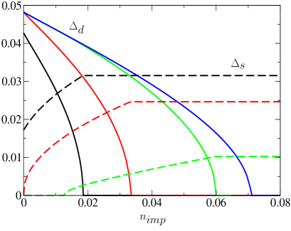
Figure 1: (color online). Superconducting gaps $\Delta_{d}$ (continous lines) and $\Delta_{s}$ (broken lines) as a function of $n_{{{\mathrm{imp}}}}$ for various values, from left to right, of the $s$-wave pairing $V_{s}=-0.45$ (mixed region), $V_{s}=-0.40$ ($s\rightarrow s+id$ critical point), $V_{s}=-0.3$ (clean $d$ phase with $s$ component induced by disorder) and $V_{s}=-0.1$ (pure $d$ phase). Here $V_{d}=-1.0$ is fixed and the inverse temperature is taken as $\beta=1000$.

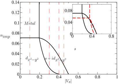
Figure 2: (color online). Phase diagram ($|V_{s}|$,$n_{{{\mathrm{imp}}}}$) of the dirty $s+id_{x^{2}-y^{2}}$ superconductor for $\beta=1000$. Thin dashed lines refer to the gaps plotted in Fig. 1. The inset illustrates the evolution of the phase boudaries with temperature, here shown for $\beta=100$ (broken lines) and $\beta=1000$ (continuous lines).

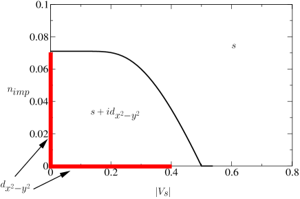
Figure 3: (color online). Zero-temperature phase diagram ($|V_{s}|$,$n_{{{\mathrm{imp}}}}$) in the dirty $s+id_{x^{2}-y^{2}}$ case. The thick line stands for the limited pure $d_{x^{2}-y^{2}}$ region. Compare with the finite temperature plot displayed in the inset of Fig. 2.

II.5 Results for the $d_{xy}+id_{x^{2}-y^{2}}$ case

II.5.1 Clean limit

In the absence of disorder, $d_{xy}$ and $d_{x^{2}-y^{2}}$ order parameters compete as in the previous case, leading to a pure $d_{x^{2}-y^{2}}$-wave state at small $V_{xy}$, a pure $d_{xy}$-wave state at large $V_{xy}$ and a mixed region of $d_{xy}+id_{x^{2}-y^{2}}$ symmetry in between (the $d_{xy}+d_{x^{2}-y^{2}}$ state being unfavorable energetically). This region is found to be given by the condition (see Appendix A):

$$\frac{|V_{d}|}{1+N_{0}|V_{d}|/2}<|V_{xy}|<\frac{|V_{d}|}{1-N_{0}|V_{d}|/2}.$$ (31)

Of course, neither the pure $d_{xy}$ phase nor the pure $d_{x^{2}-y^{2}}$ phase obey Anderson’s theorem. This will have important consequences for the following analysis.

II.5.2 $d_{xy}$-wave instability in a dirty $d_{x^{2}-y^{2}}$-wave background

We now consider the effect of a small pairing amplitude in the $d_{xy}$ channel, supposing that the $d_{x^{2}-y^{2}}$ order is present despite the finite amount of disorder. Although a finite density of states $\rho_{0}$ is present, we easily see that the naive argument predicting a weak-coupling BCS instability for the $\Delta_{xy}$ gap does not hold. Indeed the gap equation (LABEL:gap1_did) in the $d_{xy}$ channel reads:

$$\Delta_{xy}=-\frac{1}{\beta}\sum_{n}^{\;\;\;\;\;\;\;\prime}2N_{0}\;V_{xy}\;\Delta_{xy}\frac{\sqrt{\Delta_{d}^{2}+\widetilde{\omega}^{2}}}{\Delta_{d}^{2}-\Delta_{xy}^{2}}\bigg{[}F(y)-E(y)\bigg{]}.$$ (32)

The integral is completely regular at low frequency, and $\Delta_{xy}$ can be put to zero, leading to a critical interaction $V_{xy}$ to generate the $d_{xy}$-wave gap, similarly to the clean case. The physics is therefore very different from the $s+id_{x^{2}-y^{2}}$ situation, and is due to the absence of Anderson’s theorem in $d_{xy}$-wave superconductors.

II.5.3 Phase diagram

The previous discussion implies that the results for the $d_{xy}+id_{x^{2}-y^{2}}$ case are markedly different from the one obtained in the $s+id_{x^{2}-y^{2}}$ case. Indeed, the numerical solution of the mean-field equations show that, if the $d_{xy}$-wave gap is not formed in the clean limit, it cannot be generated by adding impurities. By the same token, in the mixed region, both order parameters $\Delta_{d}$ and $\Delta_{xy}$ are gradually suppressed. This is shown in Fig. 4.

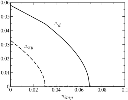
Figure 4: Superconducting gaps $\Delta_{d}$ (continous line) and $\Delta_{xy}$ (broken line) as a function of $n_{{{\mathrm{imp}}}}$ for the $d_{xy}$-wave pairing $V_{xy}=-0.47$ (mixed phase in the clean limit), with $V_{d}=-0.5$ and $\beta=100$.

The phase diagram illustrates this behavior, see Fig. 5. We stress that the zero-temperature phase diagram is quite similar to this picture, i.e., the pure $d_{x^{2}-y^{2}}$-wave region remains extended, in contrast to the $s+id_{x^{2}-y^{2}}$ case.

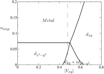
Figure 5: Phase diagram ($|V_{xy}|$,$n_{{{\mathrm{imp}}}}$) of the dirty $d_{xy}+id_{x^{2}-y^{2}}$ superconductor, with $V_{d}=-0.5$ and $\beta=100$. The thin dashed line refers to the gaps drawn in Fig. 4.

III ${\mathcal{C}}$-breaking in disordered superconductors

In contrast to conventional superconductors, cuprates derive from their Mott insulating parent compounds, and the strong-correlation physics of doped Mott insulators is responsible for many of the intriguing phenomena observed in these high-$T_{c}$ materials. Theoretical studies of microscopic models, such as the $t-J$ and Hubbard models on a two-dimensional square lattice, have shown that a variety of ordering tendencies compete, and that the actual ground state may depend sensitively on microscopic details. Experimentally, some compounds shown evidence for lattice symmetry breaking in form of charge and/or spin order, possibly coexisting with superconductivity at low temperatures.

In this section, we shall consider the competition between superconductivity and additional order associated with broken translation symmetry under the influence of disorder. Many candidates for the additional order could be chosen Vojta et al. (2000c), but we will concentrate here on the simplest case of additional bond (or spin-Peierls) order, where bond strengths are modulated as shown in Fig. 6. Such a state obeys a two-site unit cell, but up to a rotation all sites are equivalent. This justifies the application of the T-matrix approximation, based on the exact solution of a single defect, where the use of a single self energy is sufficient. In contrast, for more complicated forms of order, such as stripe states with varying site charge density, the T-matrix approach would clearly be inappropriate, and this is one of the reasons to restrict our attention to bond order.

III.1 Formalism

We start by developing the necessary formalism in the absence of disorder, then compute the T-matrix in such a non-translation-invariant superconducting background, which will finally lead us to study how disorder affects the chosen ordered state.

Figure 6: Gap structure of a bond-ordered superconductor (dubbed spin Peierls in the following). In general, gaps take complex values, so that time reversal symmetry is also broken.

III.1.1 Clean case

Contrarily to Sec. II, we cannot directly simplify the analysis in the continuum limit as the lattice symmetry is now explicitely broken. The simplest discrete model that exhibits the physics we are interested in is given by the $t-J$ Hamiltonian:

$$H_{tJ}=\sum_{{\bf R}{\bf R}^{\prime}\sigma}\left[-t_{{\bf R}{\bf R}^{\prime}}c_{{\bf R}\sigma}^{\dagger}c_{{\bf R}^{\prime}\sigma}^{\phantom{\dagger}}+J_{{\bf R}{\bf R}^{\prime}}\left({\bf S}_{{\bf R}}\cdot{\bf S}_{{\bf R}^{\prime}}-\frac{{n}_{{\bf R}}{n}_{{\bf R}^{\prime}}}{4}\right)\right]$$ (33)

where the ${c}_{{\bf R}\sigma}^{\dagger}$ operators prohibit from double occupancies, the rest of the notation being standard. Restricting both hopping $t$ and exchange interaction $J$ to nearest-neighbor sites, and introducing a slave boson $b_{{\bf R}}^{\dagger}$ to implement the non-double occupancy restriction, with the representation $c_{{\bf R}\sigma}^{\dagger}=f_{{\bf R}\sigma}^{\dagger}b_{{\bf R}}^{\phantom{\dagger}}$ and the constraint $\sum_{\sigma}f_{{\bf R}\sigma}^{\dagger}f_{{\bf R}\sigma}^{\phantom{\dagger}}+b_{{\bf R}}^{\dagger}b_{{\bf R}}^{\phantom{\dagger}}=1$, we arrive at

$$H = -t\sum_{\left<{\bf R}{\bf R}^{\prime}\right>\sigma}b_{{\bf R}}^{\phantom{\dagger}}b_{{\bf R}^{\prime}}^{\dagger}f_{{\bf R}\sigma}^{\dagger}f_{{\bf R}^{\prime}\sigma}^{\phantom{\dagger}}-\mu\sum_{{\bf R}\sigma}f_{{\bf R}\sigma}^{\dagger}f_{{\bf R}\sigma}^{\phantom{\dagger}}$$

$$- J\sum_{\left<{\bf R}{\bf R}^{\prime}\right>\sigma s}(-1)^{\sigma}f_{{\bf R}\sigma}^{\dagger}f_{{\bf R}^{\prime}-\sigma}^{\dagger}(-1)^{s}f_{{\bf R}^{\prime}-s}^{\phantom{\dagger}}f_{{\bf R}s}^{\phantom{\dagger}}$$

where $\left<{\bf R}{\bf R}^{\prime}\right>$ denotes nearest neighbor pairs of lattice sites, and $\mu$ is the chemical potential enforcing the constraint. We have organized the interaction term in such a way that the mean-field treatment in the particle-particle sector (controlled by a large-$N$ limit in the Sp($N$) formulation Sachdev and Read (1991); Vojta et al. (2000c)) is quite straightforward:

$$H_{MF} = -t_{{\mathrm{eff}}}\sum_{\left<{\bf R}{\bf R}^{\prime}\right>\sigma}f_{{\bf R}\sigma}^{\dagger}f_{{\bf R}^{\prime}\sigma}^{\phantom{\dagger}}-\mu\sum_{{\bf R}\sigma}f_{{\bf R}\sigma}^{\dagger}f_{{\bf R}\sigma}^{\phantom{\dagger}}$$

$$+ \sum_{\left<{\bf R}{\bf R}^{\prime}\right>\sigma}(-1)^{\sigma}\Delta_{{\bf R}{\bf R}^{\prime}}f_{{\bf R}\sigma}^{\dagger}f_{{\bf R}^{\prime}-\sigma}^{\dagger}+h.c.$$

with

$$\Delta_{{\bf R}{\bf R}^{\prime}} = -J\sum_{s}(-1)^{s}\big{<}f_{{\bf R}^{\prime}-s}^{\phantom{\dagger}}f_{{\bf R}s}^{\phantom{\dagger}}\big{>}$$ (36)

This mean-field is equivalent to the pairing part within the BCS formalism (which can be argued Kudo and Yamada (2004) to be enough even when pairing is induced by the presence of strong correlations). The slave bosons $b_{{\bf R}}$ in (III.1.1) condense at low temperatures, and at the mean-field level the $b_{{\bf R}}$ operators are simply replaced by their condensation amplitude $b_{{\bf R}}^{\dagger}=\big{<}b_{{\bf R}}^{\dagger}\big{>}=\sqrt{\delta}$, where $\delta$ is the hole doping, $\sum_{R\sigma}f_{{\bf R}\sigma}^{\dagger}f_{{\bf R}\sigma}^{\phantom{\dagger}}=1-\delta$. Thus, the strong Coulomb repulsion in the model (33) is accounted for by a renormalized hopping $t_{{\mathrm{eff}}}=t\delta$ in (III.1.1).

If we assume the symmetry breaking pattern shown in Fig. 6, we have two sites per unit cell. On these two sublattices, we can define the fermions $f_{{\bf R}\sigma}^{\dagger}\equiv c_{Ij\sigma}^{\dagger}$ for ${\bf R}=2I{\bf e}_{x}+j{\bf e}_{y}$ and $f_{{\bf R}\sigma}^{\dagger}\equiv d_{Ij\sigma}^{\dagger}$ for ${\bf R}=(2I+1){\bf e}_{x}+j{\bf e}_{y}$, where $I$ and $j$ are integers. Generalizing the Nambu formalism, we introduce a four-component spinor:

$$\Psi^{\dagger}\equiv(c_{K_{x}k_{y}\uparrow}^{\dagger}\;\;c_{-K_{x}-k_{y}\downarrow}^{\phantom{\dagger}}\;\;d_{K_{x}k_{y}\uparrow}^{\dagger}\;\;d_{-K_{x}-k_{y}\downarrow}^{\phantom{\dagger}})$$ (37)

with $K_{x}=2k_{x}$ the supermomentum associated to $I$ and $k_{y}$ the usual momentum associated to $j$. After some manipulations (see Appendix B), we find the mean-field Hamiltonian in matrix form $H_{MF}=\sum_{K_{x}k_{y}}\Psi^{\dagger}\hat{h}_{k}\Psi$, where:

$$\hat{h}_{k}=\left[\begin{array}[]{cccc}-2t_{{\mathrm{eff}}}\cos k_{y}-\mu&2\Delta_{3}\cos k_{y}&-t_{{\mathrm{eff}}}-t_{{\mathrm{eff}}}e^{-iK_{x}}&\Delta_{1}+\Delta_{2}e^{-iK_{x}}\\ 2\Delta_{3}^{\star}\cos k_{y}&2t_{{\mathrm{eff}}}\cos k_{y}+\mu&\Delta_{1}^{\star}+\Delta_{2}^{\star}e^{-iK_{x}}&t_{{\mathrm{eff}}}+t_{{\mathrm{eff}}}e^{-iK_{x}}\\ -t_{{\mathrm{eff}}}-t_{{\mathrm{eff}}}e^{iK_{x}}&\Delta_{1}+\Delta_{2}e^{iK_{x}}&-2t_{{\mathrm{eff}}}\cos k_{y}-\mu&2\Delta_{3}\cos k_{y}\\ \Delta_{1}^{\star}+\Delta_{2}^{\star}e^{iK_{x}}&t_{{\mathrm{eff}}}+t_{{\mathrm{eff}}}e^{iK_{x}}&2\Delta_{3}^{\star}\cos k_{y}&2t_{{\mathrm{eff}}}\cos k_{y}+\mu\end{array}\right]$$ (42)

The gap equation (36) can similarly expressed (see Appendix B) in terms of Green’s functions of the $\Psi$ spinor:

$$\hat{g}^{-1}=i\omega_{n}-\hat{h}_{k}-\hat{\Sigma}$$ (43)

where $\hat{\Sigma}$ contains effects due to the disorder distribution, that we will evaluate now. In principle, $\hat{\Sigma}$ has also contributions due to fluctuation effects beyond mean-field, which we will not take into account here.

III.1.2 Calculation of the T-matrix

The calculation of the T-matrix corresponds to solving the problem of a single localized impurity at ${\bf R=0}$ in the superconducting background state. It is obtained from the solution of the problem $H_{MF}+v\sum_{\sigma}f_{{\bf 0}\sigma}^{\dagger}f_{{\bf 0}\sigma}^{\phantom{\dagger}}$, and after some manipulations, we find (see Appendix B):

$$\hat{T}(i\omega_{n})=\frac{1}{G_{11}G_{22}-G_{12}G_{21}}\left[\begin{array}[]{cccc}-G_{22}&G_{21}&0&0\\ G_{12}&G_{11}&0&0\\ 0&0&-G_{44}&G_{43}\\ 0&0&G_{34}&G_{33}\end{array}\right]\\$$ (44)

where $G_{mn}(i\omega_{n})=\sum_{K_{x}k_{y}}g_{mn}(i\omega_{n},K_{x},k_{y})$ is the local propagator. For simplicity, we have assumed the unitary limit $v=+\infty$.

III.1.3 Self-consistency cycle

In the presence of a finite but small concentration $n_{{{\mathrm{imp}}}}$ of impurities, we can approximate the self-energy by $\hat{\Sigma}=n_{{{\mathrm{imp}}}}\hat{T}$. Self-consistency must be reached at two levels: first because the T-matrix is expressed through the propagator by the result (44) and Dyson’s equation (43), second because the gaps $\Delta_{1},\Delta_{2},\Delta_{3}$ should obey the BCS equations (53-55). This whole procedure is performed numerically, with a discrete momentum mesh and at small finite temperature.

III.2 Numerical results

III.2.1 Clean case

In the absence of disorder, the Hamiltonian (III.1.1) shows several phases as a function of the pairing attraction $J$ and doping $\delta$ Sachdev and Read (1991); Vojta et al. (2000c). The ${\mathcal{C}}$-broken bond-order phase, which coexists with superconductivity, occurs typically at low doping, and is characterized by the $\Delta_{1},\Delta_{2},\Delta_{3}$ all being different. Because the effective hopping $t_{{\mathrm{eff}}}=t\delta$ can become much smaller than $J$ in this regime, this corresponds to a strong-coupling superconductor. The bond-ordered state also breaks ${\mathcal{T}}$, as the three bond variables cannot be made all real by a global gauge transformation. At intermediate doping, the ground state is uniform, but continues to break time-reversal symmetry, as the $s^{\star}+id_{x^{2}-y^{2}}$ phase happens to be more stable (if $J$ is large enough only, otherwise the pure $d_{x^{2}-y^{2}}$-wave state with $\Delta_{1}=\Delta_{2}=-\Delta_{3}$ is found). Finally, an extended $s$-wave phase, denoted $s^{\star}$ and characterized by $\Delta_{1}=\Delta_{2}=\Delta_{3}$, is encountered at larger doping. We have checked numerically these known results for the clean case, as shown in Fig. 7.

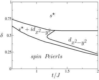
Figure 7: Superconducting phase diagram of the clean $t-J$ model for $\beta=100$ (in units of $J=1$), with a two-site unit cell. The transition from $s^{\star}$ to $d_{x^{2}-y^{2}}$ is discontinuous, whereas all other phase boundaries are second order. These results are consistent with Sachdev and Read (1991).

III.2.2 Dirty case

We investigate now how these phases evolve with the addition of non-magnetic impurities. For this model calculation, we stress that Anderson’s theorem does not hold, as a finite energy bandwidth is used (see the discussion at the end of Sec. II.2). For this reason, and in contrast to the results obtained in the first part of the paper, we do not see transitions from $d_{x^{2}-y^{2}}$ to $s^{\star}+id_{x^{2}-y^{2}}$ by increasing the disorder, and rather all superconducting phases are destroyed in a similar fashion.

Let us discuss the effect of adding impurities to the bond-ordered phase. The numerical solution of the problem demonstrates that the translation symmetry is restored during this process, i.e. the ${\mathcal{C}}$-broken phase is generically unstable to the addition of disorder, as displayed in Fig. 8.

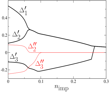
Figure 8: (color online). Superconducting gaps as a function of impurity concentration, for $t/J=1$, $\beta=100$ and $\delta=0.375$. Single (double) primed quantities denote real (imaginary) parts, respectively. Here we chose a gauge where $\Delta_{1}^{\prime}=0$. The initial state at $n_{{{\mathrm{imp}}}}=0$ is the bond-ordered superconductor described in the text.

This result can be expected on the basis that impurities disrupt the perfect arrangement of superconducting dimers, suppressing their long-range order. (In principle, it is possible that dimers locally arrange around impurities, resulting in enhanced local dimer correlations Ghosal et al. (1988), but this is not related to bond long-range order, and is certainly beyond the scope of our mean-field approach.) Discussing in more detail the evolution of the bond parameters shown in this figure, we see that the strongly dimerized superconductor persists for $0<n_{{{\mathrm{imp}}}}<0.07$, while being progressively suppressed. We then have a narrow $s^{\star}+id_{x^{2}-y^{2}}$ phase with restored lattice symmetry for $0.07<n_{{{\mathrm{imp}}}}<0.10$ (in which $\Delta_{1}^{\prime\prime}=\Delta_{2}^{\prime\prime}=0$ and $\Delta_{1}^{\prime}=\Delta_{2}^{\prime}=|\Delta_{3}^{\prime}+i\Delta_{3}^{\prime\prime}|$). Finally, a $d_{x^{2}-y^{2}}$-wave state (gaps are real, with $\Delta_{1}=\Delta_{2}=-\Delta_{3}$) is found at larger impurity concentration, ultimately unstable towards the $s^{\star}$ phase (with $\Delta_{1}=\Delta_{2}=\Delta_{3}$) for $n_{{{\mathrm{imp}}}}>0.25$ in a discontinuous manner.

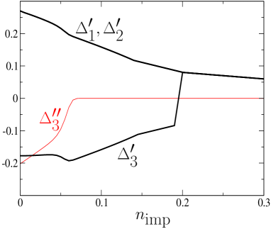
Figure 9: (color online). Superconducting gaps as a function of impurity concentration, same conditions as in Fig. 8, with $\delta=0.45$ here. The initial state at $n_{{{\mathrm{imp}}}}=0$ is $s^{\star}+id_{x^{2}-y^{2}}$.

Similarly, starting at larger doping from the clean $s^{\star}+id_{x^{2}-y^{2}}$ phase, Fig. 9 shows an initial suppression with $n_{{{\mathrm{imp}}}}$ of the ${\mathcal{T}}$-breaking towards the $d_{x^{2}-y^{2}}$-wave phase, which finally displays a first-order transition into the extended $s^{\star}$-wave phase. In all these calculations, we note that the unrealistic value for the critical concentration, where all superconductivity ultimately vanishes, is an artifact of the mean-field approximation: to stabilize the bond-ordered phase, a very small $t_{\rm eff}$ is required, placing the superconductor effectively into the strong-coupling limit which is rather robust against impurities. Nevertheless, we expect our results to correctly capture the qualitative aspects of impurity doping.

The described sequence of phases as a function of impurity concentration can roughly be guessed from the knowledge of the phase diagram in the clean case. We summarize our results for the dirty ${\mathcal{C}}$-breaking superconductor in Fig. 10. We have not mapped out the full set of phase boundaries for all possible parameter combinations, thus for different values of $t/J$, the various phases might organize themselves in a different way.

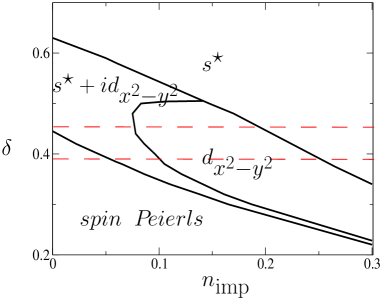
Figure 10: Superconducting phase diagram of the dirty $t-J$ model as a function of impurity concentration $n_{{{\mathrm{imp}}}}$ and doping $\delta$, for $t/J=1$ and $\beta=100$. The two dashed lines refer to the cuts in Figs. 8 and 9, respectively.

IV Discussion and conclusions

In this paper, we have investigated the influence of static disorder on superconductors with competing instabilities. Regarding the possibility of ${\mathcal{T}}$-breaking states with a mixed gap of $s+id_{x^{2}-y^{2}}$ and $d_{xy}+id_{x^{2}-y^{2}}$ structure, we found important qualitative differences between those two cases in the process of adding non magnetic impurities. In studying next a superconductor with bond long-range order (doped spin-Peierls state), we found that the lattice symmetry is very quickly recovered by addition of disorder, and we would expect this effect to be generic.

IV.1 Application to high-temperature superconductors

The finite-temperature phase diagrams displayed in Fig. 2 for the $s+id_{x^{2}-y^{2}}$ superconductor and Fig. 5 for the $d_{xy}+id_{x^{2}-y^{2}}$ superconductor show clear qualitative differences to the effect of impurity addition. Indeed, the minor $s$-component is enhanced with respect to the dominant $d_{x^{2}-y^{2}}$-wave background in the first case, whereas the small $d_{xy}$ part of the gap is very rapidly suppressed in the second case. This implies that typical tunelling spectra would evolve in a very different manner with impurity concentration, depending of the underlying structure of the superconducting gap: in the $s+id_{x^{2}-y^{2}}$ case, we expect that the zero-bias conductance peak splitting should increase, while the opposite behavior could be seen in the $d_{xy}+id_{x^{2}-y^{2}}$ case. It would thus be very interesting to see such an experimental study in overdoped YBa₂Cu₃O_7-δ, which could lead to a definite statement on the nature of the mixed superconducting gap in this compound. We recognize, however, that the practical situation might be complicated by the fact that magnetic moments can be induced by non-magnetic scatterers such as Zn Bobroff et al. (1999), which then would strongly affect the $s$-wave component as well.

A second point we would like to emphasize is that the typical coexistence windows given in equations (26) and (31) are extremely narrow in the weak-coupling regime $N_{0}V_{d}\ll 1$. Because of their smaller critical temperature, we believe that electron-doped superconductors as Pr_2-xCe_xCuO₄ fall into this condition, explaining the absence of clear observation of a mixed phase in tunneling experiments Biswas et al. (2002).

Let us turn to states with additional breaking of translation symmetry, i.e., charge order. Our calculation nicely shows that the global symmetry is restored very quickly upon adding impurities. Clearly, physics beyond mean-field can lead to the nucleation of local symmetry-breaking patterns around impurities due to pinning effects. Then, in the presence of a sufficient amount of impurity disorder, signatures of charge ordering will only be visible in local probes, such as STM, but no sharp superlattice Bragg peaks will be seen, and no thermodynamic phase transition will occur. This scenario definitely has similarities with what is seen in certain cuprate compounds McElroy et al. (2004); Vershinin et al. (2004); Howald et al. (2003).

Competing orders are ubiquitous to many exotic superconductors. Thus we think the theory developed in this paper would likely find applications in some other context. Candidate examples are Na_xCoO₂ Takada et al. (2003), a possible realization of a doped Mott insulator on the triangular lattice, and organic superconductors of the BEDT-TTF family McKenzie (1997), where both spin and charge fluctuations seems to play a crucial role for the pairing mechanism.

Appendix A Derivation of the gap equation for ${\mathcal{T}}$-breaking superconductors

A.1 $s+id_{x^{2}-y^{2}}$ superconductor

In order to set up clearly the notation, we present how the gap equations (18)-(19) can be obtained from (2). We first transform the k sums into an integral over angle and energy in the infinite bandwidth limit, allowing Anderson’s theorem to be preserved Kim and Overhauser (1993); Fay and Appel (1995):

$$\Delta_{s} = -\frac{1}{\beta}\sum_{n}^{\;\;\;\;\;\;\;\prime}\int_{0}^{2\pi}\!\!\!\frac{{{\mathrm{d}}}\phi}{2\pi}\int_{-\infty}^{+\infty}\!\!\!\!\!\!\!{{\mathrm{d}}}\epsilon\frac{N_{0}V_{s}\widetilde{\Delta}_{s}}{\widetilde{\omega}^{2}+\widetilde{\Delta}_{s}^{2}+\Delta_{d}^{2}\cos^{2}(2\phi)+\epsilon^{2}}$$

$$\Delta_{d} = -\frac{1}{\beta}\sum_{n}^{\;\;\;\;\;\;\;\prime}\int_{0}^{2\pi}\!\!\!\frac{{{\mathrm{d}}}\phi}{2\pi}\int_{-\infty}^{+\infty}\!\!\!\!\!\!\!{{\mathrm{d}}}\epsilon\frac{N_{0}V_{d}\Delta_{d}\cos^{2}(2\phi)}{\widetilde{\omega}^{2}+\widetilde{\Delta}_{s}^{2}+\Delta_{d}^{2}\cos^{2}(2\phi)+\epsilon^{2}}.$$

Because of the self-consistency, $\widetilde{\omega}$ and $\widetilde{\Delta}_{s}$ are unknown functions of the frequency $\omega_{n}$, and the Matsubara sum cannot be performed analytically. However, the integral over $\epsilon$ is straightforward to do:

$$\!\!\!\!\!\!\!\Delta_{s} = -\frac{1}{\beta}\sum_{n}^{\;\;\;\;\;\;\;\prime}\int_{0}^{\pi/2}\!\!\!\!\!\!\!{{\mathrm{d}}}\phi\frac{2N_{0}V_{s}\widetilde{\Delta}_{s}}{\sqrt{\widetilde{\omega}^{2}+\widetilde{\Delta}_{s}^{2}+\Delta_{d}^{2}\cos^{2}\phi}}\,,$$ (45)

$$\!\!\!\!\!\!\!\Delta_{d} = -\frac{1}{\beta}\sum_{n}^{\;\;\;\;\;\;\;\prime}\int_{0}^{\pi/2}\!\!\!\!\!\!\!{{\mathrm{d}}}\phi\frac{2N_{0}V_{d}\Delta_{d}\cos^{2}\phi}{\sqrt{\widetilde{\omega}^{2}+\widetilde{\Delta}_{s}^{2}+\Delta_{d}^{2}\cos^{2}\phi}}$$ (46)

which leads indeed to expressions (18)-(19).

The $1/\omega$ large frequency behavior in the Matsubara sum is due to taking the infinite bandwidth limit, and a frequency cutoff $\omega_{c}$ must be introduced. In practice we have not employed a hard cutoff, as this leads to a first-order jump of the order parameter at the critical temperature, but rather a smooth cutoff function, $\sum_{n}^{\;\;\prime}\rightarrow\sum_{n}f(\omega_{n})$, with:

$$f(\omega)=\left\{\begin{array}[]{ll}1&\mbox{if $\omega<\omega_{c}$}\\ e^{-2(\omega-\omega_{c})/\omega_{c}}&\mbox{if $\omega>\omega_{c}$}\\ \end{array}\right.\,.$$

Finally, let us determine the location of the critical points in the clean limit Musaelian et al. (1996). Subtracting twice (46) from (45) at zero temperature gives:

$$V_{s}^{-1}-2V_{d}^{-1}=2N_{0}\int_{0}^{\pi/2}\!\!\!\!\!\!\!{{\mathrm{d}}}\phi\int_{-\omega_{c}}^{\omega_{c}}\frac{{{\mathrm{d}}}\omega}{2\pi}\frac{\cos(2\phi)}{\sqrt{\omega^{2}+\Delta_{s}^{2}+\Delta_{d}^{2}\cos^{2}\phi}}$$

Performing the $\omega$-integral in the large $\omega_{c}$ limit, we find:

$$V_{s}^{-1}-2V_{d}^{-1} = -2N_{0}\int_{0}^{\pi/2}\!\!\!\!\!\!\!{{\mathrm{d}}}\phi\;\cos(2\phi)\;\log\left(\alpha^{2}+\cos^{2}\phi\right)$$ (47)

$$= \frac{N_{0}}{2}\left(-1-2\alpha^{2}+2\alpha\sqrt{\alpha^{2}+1}\right)$$

where $\alpha\equiv\Delta_{s}/\Delta_{d}$. The instability criterion for the $s$-wave phase (resp. $d_{x^{2}-y^{2}}$-wave) is given by $\alpha=0$ (resp. $\alpha=\infty$), leading to the mixed region (26).

A.2 $d_{xy}+id_{x^{2}-y^{2}}$ superconductor

The derivation of the gap equation is very similar to the previous case, and we only quote the intermediate result:

$$\Delta_{xy} = -\frac{1}{\beta}\sum_{n}^{\;\;\;\;\;\;\;\prime}\int_{0}^{\pi/2}\!\!\!\!\!\!\!{{\mathrm{d}}}\phi\frac{2N_{0}V_{xy}\Delta_{xy}\sin^{2}\phi}{\sqrt{\widetilde{\omega}^{2}+\Delta_{xy}^{2}\sin^{2}\phi+\Delta_{d}^{2}\cos^{2}\phi}}\,,$$

$$\Delta_{d} = -\frac{1}{\beta}\sum_{n}^{\;\;\;\;\;\;\;\prime}\int_{0}^{\pi/2}\!\!\!\!\!\!\!{{\mathrm{d}}}\phi\frac{2N_{0}V_{d}\Delta_{d}\cos^{2}\phi}{\sqrt{\widetilde{\omega}^{2}+\Delta_{xy}^{2}\sin^{2}\phi+\Delta_{d}^{2}\cos^{2}\phi}}$$

which gives expressions (LABEL:gap1_did)-(25) after some manipulations.

We also find the location of the critical points in the clean limit. Subtracting (LABEL:GAP2_did) from (LABEL:GAP1_did) at zero temperature and performing the $\omega$-integral at large $\omega_{c}$ leads to:

$$V_{xy}^{-1}-V_{d}^{-1}\!\!\! = \!\!\!-2N_{0}\!\!\int_{0}^{\pi/2}\!\!\!\!\!\!\!{{\mathrm{d}}}\phi\cos(2\phi)\log\left(\frac{\alpha^{2}}{1-\alpha^{2}}+\cos^{2}\phi\right)$$ (50)

$$= \frac{N_{0}}{2}\frac{\alpha-1}{\alpha+1}$$

where $\alpha\equiv\Delta_{xy}/\Delta_{d}$ now. The instability criterion for the $d_{xy}$-wave phase (resp. $d_{x^{2}-y^{2}}$-wave) is given by $\alpha=0$ (resp. $\alpha=\infty$), leading to the mixed region (31).

Appendix B Dirty superconductor with bond order

B.1 Gap equation

We give here some details on the derivation of the gap equation for the bond-ordered superconductor. Due to the broken lattice symmetry, the resulting $2\times 1$ unit cell leads us to introduce two fermion species on each sublattice, $c_{Ij\sigma}^{\dagger}$ and $d_{Ij\sigma}^{\dagger}$, and we can directly express the Hamiltonian (III.1.1) in real space in those variables. It is then convenient to go to Fourier space, and we set

$$c_{Ij\sigma}^{\dagger} = \sum_{K_{x}}\sum_{k_{y}}c_{Kxk_{y}\sigma}^{\dagger}\;e^{i(K_{x}I+k_{y}j)}\,,$$ (51)

$$d_{Ij\sigma}^{\dagger} = \sum_{K_{x}}\sum_{k_{y}}d_{Kxk_{y}\sigma}^{\dagger}\;e^{i(K_{x}I+k_{y}j)}\,,$$ (52)

where $K_{x}=2\pi/(L/2),\ldots,2\pi$ and $k_{y}=2\pi/L,\ldots,2\pi$ take respectively $L/2$ and $L$ values ($L\times L$ is the total number of sites). Inserting these expression in the mean-field Hamiltonian gives readily the final matrix expression (42).

We can also write the gap equation (36) in terms of these degrees of freedom:

$$\Delta_{1} = -\frac{J}{\beta}\sum_{\omega_{n}K_{x}k_{y}}\sum_{\sigma}(-1)^{\sigma}\big{<}d_{-K_{x}-k_{y}-\sigma}^{\phantom{\dagger}}c_{K_{x}k_{y}\sigma}^{\phantom{\dagger}}\big{>}$$

$$\Delta_{2} = -\frac{J}{\beta}\sum_{\omega_{n}K_{x}k_{y}}\sum_{\sigma}(-1)^{\sigma}e^{iK_{x}}\big{<}d_{-K_{x}-k_{y}-\sigma}^{\phantom{\dagger}}c_{K_{x}k_{y}\sigma}^{\phantom{\dagger}}\big{>}$$

$$\Delta_{3} = -\frac{J}{\beta}\sum_{\omega_{n}K_{x}k_{y}}\sum_{\sigma}(-1)^{\sigma}e^{ik_{y}}\big{<}c_{-K_{x}-k_{y}-\sigma}^{\phantom{\dagger}}c_{K_{x}k_{y}\sigma}^{\phantom{\dagger}}\big{>}$$

Introducing the propagators $g_{mn}\equiv\big{<}\Psi_{n}^{\dagger}\Psi_{m}^{\phantom{\dagger}}\big{>}$, we can write the gap equations as:

$$\Delta_{1} = -\frac{J}{\beta}\sum_{\omega_{n}K_{x}k_{y}}\big{[}g_{14}+g_{32}\big{]}$$ (53)

$$\Delta_{2} = -\frac{J}{\beta}\sum_{\omega_{n}K_{x}k_{y}}\big{[}e^{iK_{x}}g_{14}+e^{-iK_{x}}g_{32}\big{]}$$ (54)

$$\Delta_{3} = -\frac{J}{\beta}\sum_{\omega_{n}K_{x}k_{y}}2\cos k_{y}\;g_{12}$$ (55)

B.2 T-matrix

We prove here the formula (44) for the T-matrix of a bond-ordered superconductor. We consider a single impurity at site ${\bf R=0}$, and start with the exact Dyson’s equation $\big{[}i\omega-H_{MF}-v\sum_{\sigma}f_{{\bf 0}\sigma}^{\dagger}f_{{\bf 0}\sigma}^{\phantom{\dagger}}\big{]}g=1$, which we want to sandwich between two Bloch states $\big{|}k,n\big{>}$, where $k=(K_{x},k_{y})$ and $n=1,\ldots,4$ is the Nambu index. Introducing the propagator $g_{mn}(k,k^{\prime})=\big{<}k,m\big{|}g\big{|}k^{\prime},n\big{>}$, we find in matrix (Nambu) notation:

$$\big{[}i\omega-\hat{h}_{k}\big{]}\hat{g}(k,k^{\prime}) = \delta_{kk^{\prime}}+v\sum_{k^{\prime\prime}}\hat{D}\hat{g}(k^{\prime\prime},k^{\prime})$$ (56)

$$\hat{D} \equiv \left[\begin{array}[]{cccc}1&0&0&0\\ 0&-1&0&0\\ 0&0&0&0\\ 0&0&0&0\end{array}\right]$$ (61)

Performing the matrix algebra, we can solve the previous equation, and we find the local propagator:

$$\hat{G}(k,k^{\prime}) = \frac{\delta_{kk^{\prime}}}{i\omega-\hat{h}_{k}}+\frac{1}{i\omega-\hat{h}_{k}}\hat{T}(i\omega)\frac{1}{i\omega-\hat{h}_{k^{\prime}}}$$ (62)

$$\hat{T}(i\omega) = v\hat{D}\left(1-v\sum_{k}\frac{1}{i\omega-\hat{h}_{k}}\hat{D}\right)^{-1}$$ (63)

$$= \frac{1}{{{\mathrm{Det}}}}\left[\begin{array}[]{cccc}-v^{-1}-G_{22}&G_{21}&0&0\\ G_{12}&v^{-1}+G_{11}&0&0\\ 0&0&0&0\\ 0&0&0&0\end{array}\right]$$ (68)

where we have defined:

$${{\mathrm{Det}}} \equiv G_{11}G_{22}-G_{12}G_{21}-v^{-1}\big{(}G_{11}+G_{22}\big{)}-v^{-2}$$

Taking into account the contribution from site ${\bf R}={\bf e}_{x}$, and in the unitary limit $v=\infty$, we find the final expression (44).

References

• Tsuei and Kirtley (2000) C. Tsuei and J. Kirtley, Rev. Mod. Phys.  72, 174507 (2000).
• Hu (1994) C. R. Hu, Phys. Rev. Lett.  72, 1526 (1994).
• Dagan and Deutscher (2001) Y. Dagan and G. Deutscher, Phys. Rev. Lett.  87, 177004 (2001).
• Sharoni et al. (2002) A. Sharoni, O. Millo, A. Kohen, Y. Dagan, R. Beck, G. Deutscher, and G. Koren, Phys. Rev. B 65, 134526 (2002).
• Wei et al. (1998) J. Y. T. Wei, N. C. Yeh, D. F. Garrigus, and M. Strasik, Phys. Rev. Lett.  81, 2542 (1998).
• Matsumoto and Shiba (1995) M. Matsumoto and H. Shiba, J. Phys. Soc. Jp. 64, 3384 (1995).
• Sigrist (1998) M. Sigrist, Prog. Theo. Phys. 99, 899 (1998).
• Sachdev and Read (1991) S. Sachdev and N. Read, Int. J. Mod. Phys. 5, 219 (1991).
• Sangiovanni et al. (2003) G. Sangiovanni, M. Capone, S. Caprara, C. Castellani, C. DiCastro, and M. Grilli, Phys. Rev. B 67, 174507 (2003).
• Laughlin (1998) R. B. Laughlin, Phys. Rev. Lett.  80, 5188 (1998).
• Balatsky (1998) A. V. Balatsky, Phys. Rev. Lett.  80, 1972 (1998).
• Vojta et al. (2000a) M. Vojta, Y. Zhang, and S. Sachdev, Phys. Rev. Lett.  85, 4940 (2000a).
• Vojta et al. (2000b) M. Vojta, Y. Zhang, and S. Sachdev, Int. J. Mod. Phys, 14, 3719 (2000b).
• Valla et al. (1999) T. Valla, A. V. Fedorov, P. D. Johnson, B. O. Wells, S. L. Hulbert, Q. Li, G. D. Gu, and N. Koshizuka, Science 285, 2110 (1999).
• Biswas et al. (2002) A. Biswas, P. Fournier, M. M. Qazilbash, V. N. Smolyaninova, H. Balci, and R. L. Greene, Phys. Rev. Lett.  88, 207004 (2002).
• Skinta et al. (2002) J. A. Skinta, M.-S. Kim, T. R. Lemberger, T. Greibe, and M. Naito, Phys. Rev. Lett.  88, 207005 (2002).
• Zaanen and Gunnarsson (1989) J. Zaanen and O. Gunnarsson, Phys. Rev. B 40, 7391 (1989).
• Vojta et al. (2000c) M. Vojta, Y. Zhang, and S. Sachdev, Phys. Rev. B 62, 6721 (2000c).
• Affleck and Marston (1988) I. Affleck and J. B. Marston, Phys. Rev. B 37, 3774 (1988).
• Tranquada et al. (1995) J. M. Tranquada, B. J. Sternlieb, J. D. Axe, Y. nakamura, and S. Uchida, Nature 375, 561 (1995).
• McElroy et al. (2004) K. McElroy, D.-H. Lee, J. E. Hoffman, K. M. Lang, E. W. Hudson, H. Eisaki, S. Uchida, J. Lee, and J. Davis (2004), eprint cond-mat/0404005.
• Vershinin et al. (2004) M. Vershinin, S. Misra, S. Ono, Y. Abe, Y. Ando, and A. Yazdani, Science 303, 1995 (2004).
• Howald et al. (2003) C. Howald, H. Eisaki, N. Kaneko, M. Greven, and A. Kapitulnik, Phys. Rev. B 67, 014533 (2003).
• Anderson (1959) P. W. Anderson, J. Chem. Phys. Solids 11, 46 (1959).
• Hirschfeld et al. (1988) P. J. Hirschfeld, P. Wölfle, and D. Einzel, Phys. Rev. B 37, 83 (1988).
• Hirschfeld and Atkinson (2002) P. J. Hirschfeld and W. A. Atkinson, J. Low. Temp. Phys 126, 881 (2002).
• Ghosal et al. (1988) A. Ghosal, M. Randeria, and N. Trivedi, Phys. Rev. Lett.  81, 3940 (1988).
• Xu et al. (1996) W. Xu, W. Kim, Y. Ren, and C. S. Ting, Phys. Rev. B 54, 12693 (1996).
• Golubov and Mazin (1997) A. A. Golubov and I. I. Mazin, Phys. Rev. B 55, 15146 (1997).
• Meyer et al. (2003) J. S. Meyer, I. V. Gornyi, and A. Altland, Phys. Rev. Lett.  90, 107001 (2003).
• Musaelian et al. (1996) K. A. Musaelian, J. Betouras, A. V. Chubukov, and R. Joynt, Phys. Rev. B 53, 3598 (1996).
• Lee (1993) P. A. Lee, Phys. Rev. Lett.  71, 1887 (1993).
• Press et al. (1988) W. H. Press, S. A. Teukolsky, W. T. Vetterling, and B. P. Flannery, Numerical recipes (Cambridge University Press, 1988).
• Kim and Overhauser (1993) Y. J. Kim and A. W. Overhauser, Phys. Rev. B 47, 8025 (1993).
• Fay and Appel (1995) D. Fay and J. Appel, Phys. Rev. B 51, 15604 (1995).
• Gorkov and Kalugin (1985) L. P. Gorkov and P. A. Kalugin, JETP Lett. 41, 253 (1985).
• Kudo and Yamada (2004) K. Kudo and K. Yamada (2004), eprint cond-mat/0403354.
• Bobroff et al. (1999) J. Bobroff, W. A. MacFarlane, H. Alloul, P. Mendels, N. Blanchard, G. Collin, and J. F. Marucco, Phys. Rev. Lett.  83, 4381 (1999).
• Takada et al. (2003) K. Takada, H. Sakurai, E. Takayama-Muromachi, F. Izumi, R. A. Dilanian, and T. Sasaki, Nature 422, 53 (2003).
• McKenzie (1997) R. H. McKenzie, Science 278, 820 (1997).