STOCHASTIC MODELS OF LAGRANGIAN ACCELERATION OF FLUID PARTICLE IN DEVELOPED TURBULENCE

Abstract

Modeling statistical properties of motion of a Lagrangian particle advected by a high-Reynolds-number flow is of much practical interest and complement traditional studies of turbulence made in Eulerian framework. The strong and nonlocal character of Lagrangian particle coupling due to pressure effects makes the main obstacle to derive turbulence statistics from the three-dimensional Navier-Stokes equation; motion of a single fluid-particle is strongly correlated to that of the other particles. Recent breakthrough Lagrangian experiments with high resolution of Kolmogorov scale have motivated growing interest to acceleration of a fluid particle. Experimental stationary statistics of Lagrangian acceleration conditioned on Lagrangian velocity reveals essential dependence of the acceleration variance upon the velocity. This is confirmed by direct numerical simulations. Lagrangian intermittency is considerably stronger than the Eulerian one. Statistics of Lagrangian acceleration depends on Reynolds number. In this review we present description of new simple models of Lagrangian acceleration that enable data analysis and some advance in phenomenological study of the Lagrangian single-particle dynamics. Simple Lagrangian stochastic modeling by Langevin-type dynamical equations is one the widely used tools. The models are aimed particularly to describe the observed highly non-Gaussian conditional and unconditional acceleration distributions. Stochastic one-dimensional toy models capture main features of the observed stationary statistics of acceleration. We review various models and focus in a more detail on the model which has some deductive support from the Navier-Stokes equation. Comparative analysis on the basis of the experimental data and direct numerical simulations is made.

1 Introduction

In fluid mechanics, acceleration can be defined as the substantive derivative of the velocity,

$$a_{i}=\frac{dv_{i}}{dt}\equiv\partial_{t}v_{i}+v_{k}\partial_{k}v_{i}.$$ (1)

When treated in Eulerian framework, acceleration incorporates the Eulerian local acceleration $\partial_{t}v_{i}$ and the nonlinear advection term $v_{k}\partial_{k}v_{i}$ which require measurements of the velocity $v_{i}$ and temporal and spatial velocity derivatives $\partial_{t}v_{i}$ and $\partial_{k}v_{i}$ at fixed point of a flow. Here, $\partial_{k}=\partial/\partial x^{k}$ denotes spatial derivative in the laboratory Cartesian frame of reference, $\partial_{t}=\partial/\partial t$ is time derivative, $i,k=1,2,3$, and summation over repeated indices is assumed.

Using Eq. (1) the three-dimensional (3D) Navier-Stokes equation for an incompressible flow can be written as

$$a_{i}=-\rho^{-1}\partial_{i}p+\nu\partial^{2}_{k}v_{i}+f_{i},$$ (2)

where $\rho$ is the constant fluid density, $p$ is the pressure, $\nu$ is the kinematic viscosity, $v_{i}$ is the velocity field, and $f_{i}$ is the forcing, which usually occurs at large characteristic spatial scale.

Measurement of time series $x_{i}(t)$ of the position of individual tracer particle and using a finite-difference scheme allows one to evaluate its Lagrangian velocity $u_{i}(t)$ and acceleration $a_{i}(t)$ as functions of time due to the Lagrangian relations

$$u_{i}(t)=\partial_{t}x_{i}(t),\quad a_{i}(t)=\partial^{2}_{t}x_{i}(t).$$ (3)

Here, $x_{i}=X_{i}(x_{0k},t)$ is the coordinate of an infinitesimal fluid particle viewed as a function of the initial position $x_{0i}\equiv x_{i}(0)$ of the particle and time $t\in[0,\infty)$. With the initial data points $x_{0i}$ (Lagrangian coordinates) running over all the fluid particles one gets a Lagrangian description of fluid flow.

In the Eulerian framework, contributions of the viscous term and the forcing are known to be small as compared to that of the pressure gradient term for a certain range of scales in a locally isotropic turbulence. Direct analytical evaluation of the Lagrangian acceleration $a_{i}(x_{0k},t)$ by using the 3D Navier-Stokes equation for high-Reynolds-number (high-Re) turbulent flows is out of reach at present. Thus one is led to estimate it theoretically in some fashion.

Accurate evaluation of the Lagrangian velocity and acceleration in laboratory turbulence experiments requires measurement of positions of neutrally buoyant tracer particle by using some tracking system to a very high accuracy. One can also use direct measurement of the Lagrangian velocity when knowing a precise position of tracer particle is not important. In any case, to get Lagrangian acceleration one should have experimental access to time scales smaller than the Kolmogorov time scale $\tau_{\eta}$ of the flow. One expects that such experimental data give information on the pressure gradient term, which is difficult to measure experimentally.

Growing interest in studying Lagrangian turbulence is motivated by the recent breakthrough Lagrangian experiment by La Porta, Voth, Crawford, Alexander, and Bodenschatz[1] (2001), the new data by Crawford, Mordant, Bodenschatz, and Reynolds[2] (2002), Mordant, Crawford, and Bodenschatz[3] (2003) (optical tracking system, $R_{\lambda}=690$, the measured acceleration range is $|a|/\langle a^{2}\rangle^{1/2}\leq 60$, and $\tau_{\eta}$ is resolved), Mordant, Delour, Leveque, Arneodo, and Pinton[4] (2002) (acoustic tracking system, $R_{\lambda}=740$, $|a|/\langle a^{2}\rangle^{1/2}\leq 20$, and $\tau_{\eta}$ is not resolved), and direct numerical simulations (DNS) of the 3D Navier-Stokes equation by Gotoh, Fukayama, and Nakano[5] (2002), Kraichnan and Gotoh[6] (2003) ($R_{\lambda}=380$, $|a|/\langle a^{2}\rangle^{1/2}\leq 150$) and Biferale, Boffetta, Celani, Lanotte, and Toschi[7] (2004) ($R_{\lambda}=280$, $|a|/\langle a^{2}\rangle^{1/2}\leq 80$, $\tau_{\eta}$ is resolved). Experimental results on the 3D Lagrangian acceleration have been reported by Mordant, Crawford, and Bodenschatz.[8] The classical Reynolds number Re is related to the Taylor microscale Reynolds number due to $\mathrm{Re}=R_{\lambda}^{2}/15$. These experiments and DNS give an important information on single-particle dynamics and statistics, and new look to the intermittency in high-Re fluid turbulence.

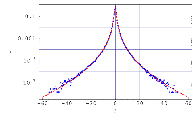
Figure 1: Lin-log plot of the Lagrangian acceleration probability density function $P(a)$ for the transverse component of acceleration. Dots: experimental data for the $R_{\lambda}=690$ flow by Crawford, Mordant, Bodenschatz, and Reynolds.² Dashed line: the stretched exponential fit (4). The acceleration component $a$ is normalized to unit variance.

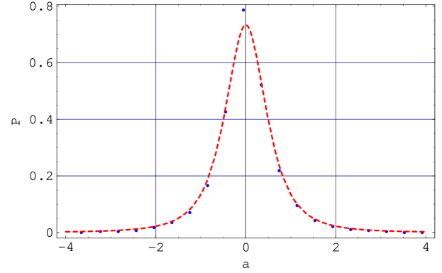
Figure 2: Lin-lin plot of the central part of the Lagrangian acceleration probability density function $P(a)$ for the transverse component of acceleration. Same notation as in Fig. 1.

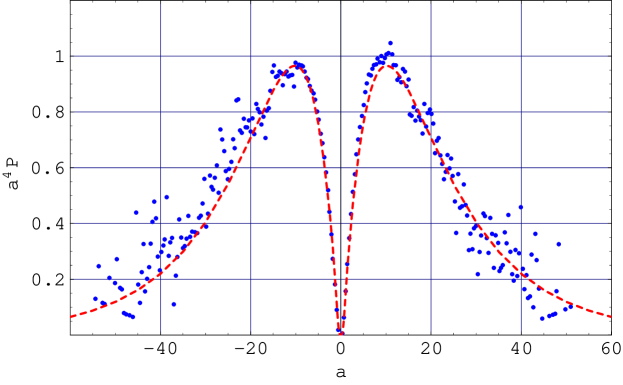
Figure 3: The contribution to fourth-order moment of Lagrangian acceleration, $a^{4}P(a)$. Same notation as in Fig. 1.

The experimental data on a component of Lagrangian acceleration $a$ of polystyrene tracer particle in the $R_{\lambda}=690$ water flow generated between two counter-rotating disks reveal that the acceleration varies with time in a wild way. Statistical description of the acceleration is then used and a huge amount of collected data have been fitted to a good accuracy by the probability density function of a stretched exponential form[1, 2, 3]

$$P(a)=C\exp\left[-\frac{a^{2}}{(1+\left|{b_{1}a}/{b_{2}}\right|^{b_{3}})b_{2}^{2}}\right].$$ (4)

Here, $b_{1}=0.513\pm 0.003$, $b_{2}=0.563\pm 0.02$, and $b_{3}=1.600\pm 0.003$ are fit parameters, and $C=0.733$ is the normalization constant.

Two coordinates $z$ and $x$, one along the large-scale symmetry axis and the other transverse to it, were measured, while the third coordinate $y$ was taken statistically equivalent to the measured transverse component. Lagrangian particles are tracked in a small central part of the flow where, in general, high degree of statistical isotropy of small scales is expected due to Kolmogorov 1941 (K41) local isotropy hypothesis.[9] The studied statistically stationary flow is highly anisotropic at large scales due to the used specific stirring mechanism. This appears to affect very small scales. Namely, one can observe small skewness of the acceleration distribution and anisotropy of the acceleration variance, as well as difference in distributions of components of Lagrangian velocity.

At large acceleration magnitudes, tails of the fitted model distribution (4) decay very slowly, asymptotically as $\exp[-|a|^{0.4}]$, which implies finitness of the acceleration fourth-order moment $\langle a^{4}\rangle=\int_{-\infty}^{\infty}a^{4}P(a)da$, as confirmed by the experiment.[2] The flatness factor of the distribution (4) which characterizes widening of its tails (when compared to a Gaussian) is $F\simeq 55.1$, which is in agreement with the experimental value

$$F\equiv{\langle a^{4}\rangle}/{\langle a^{2}\rangle^{2}}=55\pm 8.$$ (5)

Gaussian distribution is characterized by much smaller value $F=3$.

The Kolmogorov time scale of the $R_{\lambda}=690$ flow is $\tau_{\eta}=0.93$ ms. Experimental resolution of the scale is very accurate, about 1/65 of $\tau_{\eta}$. Low-pass filtering with the 0.23$\tau_{\eta}$ width of the collected $1.7\times 10^{8}$ data points was used, and the response time of optically tracked 46 $\mu$m diameter tracer particle is 0.12$\tau_{\eta}$. Note that certain nonzero time scale less than the Kolmogorov time scale is used to derive Lagrangian velocity and acceleration values. The width of filter has a limited impact on the resulting value of $F$, e.g. the use of 0.31$\tau_{\eta}$ width results in about 15% decrease of the experimental value of flatness $F$. Notice that non-ideal response characteristics of tracer particle may result in an increase of the effective integral time scale, from the Lagrangian integral time scale $T_{L}$ to the Eulerian integral time scale $T_{E}$ (calculated in the comoving frame), as one can show by using Corrsin hypothesis.[10]

The experimental data and stretched exponential fits are shown in Figs. 1, 2 and 3. One can observe almost symmetric distributions with respect to zero acceleration and very intermittent character of the Lagrangian acceleration. Namely, the pronounced central peak (low accelerations) and long tails (high accelerations) make a highly non-Gaussian shape of the acceleration distribution shown in Fig. 1. One concludes that the observed fluid-particle dynamics is featured by relatively frequent acceleration bursts, up to the measured 60 standard deviations. Such extreme events occur when the tracer particle is captured by intense small-scale vortical structures which are thought to be present in the turbulent flow. These structures seem to be distributed randomly in space and time, with large intervals between them which are characterized by low-intensity events. As shown by Farge, Pellegrino, and Schneider[11] the most of the turbulent kinetic energy is carried by vortex tubes, which are surrounded by a background incoherent flow.

The long-standing Heisenberg-Yaglom scaling of a component of Lagrangian acceleration,[12, 13]

$$\langle a^{2}\rangle=a_{0}{\bar{u}}^{9/2}\nu^{-1/2}L^{-3/2},$$ (6)

was confirmed experimentally[1] to a high accuracy, for about seven orders of magnitude in the acceleration variance, or two orders of the root-mean-square (rms) velocity $\bar{u}=\langle u^{2}\rangle^{1/2}$ ($500\leq R_{\lambda}\leq 980$). Here, the Lagrangian velocity $u$ is such that the average $\langle u\rangle=0$, $a_{0}$ is the Kolmogorov constant, $\nu$ is the kinematic viscosity, and $L$ is the Lagrangian integral length scale. For $R_{\lambda}<500$ the Heisenberg-Yaglom scaling was found to be broken. This signals increasing coupling of the acceleration to large scales of the flow, and may be related specifically to the large-scale anisotropy effect or to “insufficient” developing of the turbulence, or to both of them.

Very recent experimental data[8] on the 3D Lagrangian acceleration in turbulent flows with $R_{\lambda}=285,485$, and 690 show that the three components $a_{x}$, $a_{y}$, and $a_{z}$ of the acceleration are statistically dependent. For example, the conditional variance $\langle a_{y}^{2}|a_{z}\rangle$ increases strongly with the magnitude of $a_{z}$. The acceleration magnitude $|\bm{a}|$ was found to be characterized by the probability density function, which is comparable to a log-normal distribution of variance 1 at small and medium values $|\bm{a}|/(\langle|{\bm a}|^{2}\rangle-\langle|{\bm a}|\rangle^{2})^{1/2}\leq 25$, and by the autocorrelation time of about the integral time scale. The autocorrelation time of the direction of the acceleration vector $\bm{a}$ is of the dissipation time scale. The observed two-time-scale character of the stochastic dynamics is consistent with previous experimental and DNS results.[4] Assuming the log-normal distribution of the magnitude $|\bm{a}|$ and statistical isotropy of the acceleration vector $\bm{a}$ one can straightforwardly derive distribution of each component[8]

$$P(a_{i})=\frac{\exp[s^{2}/2]}{4m}\left[1-\mbox{erf}\left(\frac{\ln[|a_{i}|/m]+s^{2}}{2s^{2}}\right)\right],$$ (7)

where erf$(x)$ is the error function, $m=\sqrt{3/e^{2s^{2}}}$ for a unit variance and $s$ is a free parameter. It was shown that the predicted distribution at $s=1$ follows experimental data points to a good accuracy at small and medium accelerations $|a_{i}|/\langle a_{i}^{2}\rangle^{1/2}\leq 25$, and overestimates them at higher values. The origin of this departure is not clear. However, it should be noted that for higher $R_{\lambda}$ tails of the observed distributions become wider, and approach the predicted curve.

It should be emphasized that the Lagrangian velocity components for the studied flow follow Gaussian distribution to a good accuracy. Theoretically, time derivative of a dynamical variable does not necessarily follow the same statistical distribution as that of the variable. The link between these two sharply distinct distributions —Lagrangian velocity and acceleration— can be seen from studying stationary statistics of the time increment of a component $u$ of the velocity of individual fluid particle,

$$\delta_{\tau}u(t)=u(t+\tau)-u(t).$$ (8)

For the time scale $\tau$ of the order of Lagrangian integral time scale $T_{L}$ (large characteristic time scale of the flow implied by simple dimensional analysis) the stationary distribution of $\delta_{\tau}u(t)$ is approximately of a Gaussian form while for $\tau$ decreasing down to the Kolmogorov time scale $\tau_{\eta}$ (small characteristic time scale of the flow implied by simple dimensional analysis) the distribution continuously develops long tails, and in a far dissipative subrange it reproduces the acceleration distribution shown in Fig. 1. For sufficiently small time scales $\tau<\tau_{\eta}$ turbulent fluctuations are smoothed, and the increment is proportional to the time scale, $\delta_{\tau}u(t)=\tau a(t)$, to a good accuracy. The ratio between the timescales, $T_{L}/\tau_{\eta}$, is very large for developed turbulent flows, and is characterized by Taylor microscale Reynolds number $R_{\lambda}$; for the studied flow it is of about two orders of magnitude.

High probability of extreme acceleration magnitudes, as compared to that implied by the corresponding Gaussian distribution, is associated with the Lagrangian turbulence intermittency, which was found to be considerably stronger than the Eulerian one. Equivalently, one can say that it is related to an increase of the probability to have larger velocity increments in time with decrease of time scale, down to the Kolmogorov one (a statistical viewpoint). This is due to the absence of the so called sweeping effect in the Lagrangian frame and the existence of relatively long-lived intense vortical structures (vortex tubes) with radii of the order of Kolmogorov length $\eta$ and total sizes extending up to the integral length scale $L$. Recent laboratory experiments by Mouri, Hori, and Kawashima[14] (see also references therein) for boundary layers with $R_{\lambda}=$ 295–1255 confirm this picture.

In the traditional Eulerian framework, the isotropic turbulence intermittency is understood differently, as an increase of the probability to have larger longitudinal velocity differences

$$\delta_{l}v(x)=v(x+l)-v(x)$$ (9)

on shorter spatial separation scales $l$, and studied through scaling exponents $\zeta^{E}(p)$ of the Eulerian velocity structure functions $\langle(\delta_{l}v)^{p}\rangle\sim\l^{\zeta^{E}(p)}$, $p=1,2,3,\ldots$ (a structural viewpoint).[15] The velocity difference is taken at the same time instance. For Lagrangian velocity structure functions one considers scaling with respect to the time scale $\tau$, $\langle(\delta_{\tau}u)^{p}\rangle\sim\tau^{\zeta(p)}$.

Scaling properties of the Eulerian and Lagrangian velocity structure functions (statistical moments of $\delta_{l}v$ and $\delta_{\tau}u$ which characterize their distributions) are traditionally used to quantify turbulence intermittency. Here, the intermittency exhibits itself as observed deviations from the “normal” scalings predicted by K41 theory. The deviations become stronger with increasing order $p$, with the exception being $\zeta^{E}(3)=1$ which corresponds to the four-fifth law by Kolmogorov ($\zeta(2)=1$ for the Lagrangian case).[9, 12]

Under the assumption of balance between the energy injected by driving forces, which occur presumably at large spatial scales, and the energy dissipated by viscous processes, which are concentrated at small scales, one can restrict consideration by a statistically steady state, and focus on intermediate scales, the inertial range, characteristics of which are universal to some extent for high-Re flows. In the inertial range the energy is transferred from large to small scales (the direct energy cascade) and viscosity effects are not noticeable. Due to the K41 hypotheses[9] certain properties of fully developed turbulence in the inertial range are independent on the details of initial conditions and forcing (boundary conditions), as well as on the details of the energy dissipation. This hypothesis is valid only statistically, in the sense that the velocity and acceleration (Heisenberg[13] and Yaglom[12]) are viewed as random variables. Hence, one is interested in probability density functions and correlators of the variables. Complete K41 scale invariance of the Eulerian velocity difference statistics is known to be broken, with the “anomaly” coming from sensitivity of the inertial range of scales to large scales of the flow. The breaking occurs also for the predicted K41 scalings of the Lagrangian velocity structure functions $\langle(\delta_{\tau}u)^{p}\rangle$ for the same reason. The observed scaling exponents behave as nonlinear functions of the order $p$ rather than linear (“normal”) ones. This is associated in general with the so called dissipative anomaly (mean turbulent kinetic energy dissipation rate remains finite when one puts the viscosity parameter to zero) corresponding to a strongly nonlinear and non-equilibrium character of a high-Re turbulent system. Possibility to describe high-Re turbulence on the basis of unified statistical principles, such as those successfully applied to (quasi-)equilibrium systems, is an open problem. The strong and nonlocal character of Lagrangian particle coupling due to pressure effects makes the main obstacle to derive turbulence statistics from the Navier-Stokes equation; motion of a single fluid-particle is strongly correlated to that of the other particles. Studying and accurate modeling Lagrangian dynamics of a many-particle configuration,[16] and particularly single-particle behavior, is currently under elaboration.

In the inertial range, which extends much for high-Re flows, contribution of the pressure gradient to the acceleration variance strongly dominates over that of the viscous force. The two contributions do not correlate and the acceleration field can be then approximated as the potential one. The DNS pressure gradient data meet that of the experimental Lagrangian acceleration.[1, 2, 6] The effects of viscosity and intermittency are known to reduce the effective inertial range characterized by the ascribed scaling.[17]

Statistical isotropy and homogeneity of a fully developed turbulent flow at small scales are assumed by K41 theory and greatly simplify statistical description of turbulence. Turbulence intermittency is related to a non-Gaussian statistical behavior and is a more subtle matter for theoretical study. Intermittency of the stochastic energy dissipation rate at scale $l$ is related to intermittency of dynamics of the system that makes a link between the Eulerian and Lagrangian aspects of intermittency. It should be emphasized that Eulerian and Lagrangian approaches in studying fluid flows are characterized by different theoretical technique and implications, and compliment each other.

Modeling statistical turbulence in the Lagrangian frame is important both for theoretical implications and applicational studies. Simple models focus on single-particle statistical properties and employ Langevin-type equations for one variable. Partial justification of the use of one-dimensional models comes from the K41 assumption on statistical isotropy of the flow at small scales. Away from boundaries one can also use the assumption on homogeneity of the flow and discard dependence of the Lagrangian tracer on initial position for a sufficiently long evolution. When comparing to the experimental or DNS data one usually peaks up one measured component of the variable, or uses averaging over all accessible components to get higher statistics. Experimentally, a three-dimensional picture is difficult to reach[8] while DNS naturally gives a full access to it. Some Lagrangian experiments allow very accurate resolution of the Kolmogorov time scale with relatively short integration time, the others allow to follow individual particle for long time but do not resolve the Kolmogorov time scale. DNS is characterized by a high resolution of the Kolmogorov time scale and long integration time but at lower $R_{\lambda}$ achieved because of current computational limitations.

As the experiments and performed DNS (on cubic lattices) do not provide perfect isotropy of large-scale forcing (boundary) one naturally expects anisotropy effects at all scales. However, these effects are usually small at small scales (even when strong large-scale anisotropy of a high-Re turbulent flow is present) and thus can be ignored in the first approximation. Influence of anisotropy effects is usually treated as a small correction. Local isotropy of a fully developed turbulent flow —rather strong but very fruitful condition— is one of the main assumptions of K41 phenomenological theory.[12] However, anisotropy effects at small scales are known to be persistent for high Reynolds numbers. For example, persistent anisotropy in the skewness of velocity derivatives in homogeneous shear flows, which represent one of the simplest anisotropic flow, is observed.[18] We remind that the forceless 3D Navier-Stokes equation is invariant under SO(3) rotational Lie group in coordinate space, and symmetry breaking may come only due to the forcing and/or boundary conditions. Recently developed SO(3) decomposition theory[19] can be used to treat anisotropic and isotopic sectors in a rigorous way, and to study how the isotropy recovery at small scales happens in Navier-Stokes turbulence. The isotropy recovery is partially justified owing to a subleading character of anisotropy found in some exactly solvable models.

Two-time-scale stochastic dynamics in describing the Lagrangian acceleration component jointly with the Lagrangian velocity and position of a fluid particle was proposed long time ago by Sawford.[20] The model equations are

$$\partial_{t}a=-(T_{L}^{-1}+\tau_{\eta}^{-1})a+T_{L}^{-1}\tau_{\eta}^{-1}u\\ +\sqrt{2\sigma_{u}^{2}(T_{L}^{-1}+\tau_{\eta}^{-1})T_{L}^{-1}\tau_{\eta}^{-1}}L(t),$$

$$\partial_{t}u=a,\quad\partial_{t}x=u,$$ (10)

where

$$T_{L}=\frac{2\sigma_{u}^{2}}{C_{0}{\bar{\epsilon}}},\quad\tau_{\eta}=\frac{C_{0}\nu^{1/2}}{2a_{0}{\bar{\epsilon}}^{1/2}}$$ (11)

are two time scales, $T_{L}\gg\tau_{\eta}$, $L(t)$ is zero-mean Gaussian-white noise, $C_{0}$ and $a_{0}$ are Lagrangian structure constants, $\sigma_{u}^{2}$ is the variance of velocity distribution, and $\bar{\epsilon}$ is the mean turbulent kinetic energy dissipation rate per unit mass.

K41 hypotheses of locally isotropic character of high-Re turbulence and similarity lead to the result that the acceleration field is spatially isotropic, $\langle a_{i}a_{j}\rangle\simeq\delta_{ij}$, and the stationary probability distribution of acceleration may depend only on the parameters $\bar{\epsilon}$ and $\nu$ (mean energy flux and viscosity). The second-order Lagrangian velocity structure function $\langle\delta_{\tau}u_{i}\delta_{\tau}u_{j}\rangle\simeq\delta_{ij}$ also should show spatial isotropy for the inertial range of time scales. Thus, a single-component consideration makes a sense; $u=u_{1},u_{2},$ or $u_{3}$ and $a=a_{1},a_{2},$ or $a_{3}$, in laboratory Cartesian frame of reference. The constant $C_{0}$ enters the linear scaling of the velocity structure function $\langle(\delta_{\tau}u)^{2}\rangle=C_{0}\bar{\epsilon}\tau$ implied by K41 theory for the inertial range of time scales $\tau_{\eta}\ll\tau\ll T_{L}$. Since the form of this two-time correlator is similar to that of the displacement of usual Brownian particle, the velocity of fluid particle in the inertial range can be thought of as a Brownian-like motion with the “diffusion” coefficient $C_{0}\bar{\epsilon}$. In other words, the velocity is a stationary stochastic process with independent increments. For time scales smaller than the Kolmogorov time scale $\tau_{\eta}$ the predicted scaling is quite different, $\langle(\delta_{\tau}u)^{2}\rangle=a_{0}\bar{\epsilon}^{3/2}\nu^{-1/2}\tau^{2}$, and directly corresponds to Heisenberg-Yaglom scaling law (6); $\bar{\epsilon}={\bar{u}}^{3}/L$, $\eta=(\nu^{3}/{\bar{\epsilon}})^{1/4}$, and $R_{\lambda}=(15/{\bar{\epsilon}}\nu)^{1/2}{\bar{u}}^{2}$. This theory also predicts ${\bar{\epsilon}}/\tau$ decay of the autocorrelation of acceleration component $\langle a(t)a(t+\tau)\rangle$, when one imposes its independence on $\nu$, for time scales $\tau$ much bigger than $\tau_{\eta}$. For the velocity autocorrelation $\langle u(t)u(t+\tau)\rangle$ the prediction is that it decays considerably only for $\tau$ of the order of Lagrangian integral time scale $T_{L}$. The uncorrelated character of Lagrangian acceleration then could be used to build a first approximation for time scales within the inertial range. Note however that the predicted decay of $\langle a(t)a(t+\tau)\rangle$ across this range is rather slow. Qualitatively K41 relations mean that the components of Lagrangian acceleration and velocity are associated mainly with small and large scales of a developed turbulent flow respectively.

Sawford model (1) predicts stationary Gaussian distributions for both the acceleration and velocity reflecting the used uncorrelated character of fluctuations and is consistent with K41 picture. One of the extensions of this model is due to replacement of $\bar{\epsilon}$ by stochastic energy dissipation rate $\epsilon$, and assuming that it is lognormally distributed in correspondence to the refined Kolmogorov 1962 (K62) approach.[21] Such extensions can be used to fit the observed highly non-Gaussian shape of the acceleration distribution shown in Fig. 1.

Recent Lagrangian experiments and DNS by Mordant, Delour, Leveque, Arneodo, and Pinton[4] and DNS by Chevillard, Roux, Leveque, Mordant, Pinton, and Arneodo[23] show that certain long-time correlations and the occurrence of very large fluctuations at small scales dominate the motion of a fluid particle, and this leads to a new dynamical picture of turbulence. This requires effective models on how to account for the specific long-time correlations along a particle trajectory which are viewed as a key to intermittency in turbulence.

While it is evident that the 3D Navier-Stokes equation with a Gaussian-white random forcing belongs to a class of non-linear stochastic dynamical equations for the velocity field with which one can associate some generalized Fokker-Planck equations or apply a path-integral method, it is a theoretical challenge to make a link between the Navier-Stokes equation (2) and phenomenological stochastic models of Lagrangian acceleration.

Recent approach by Friedrich[24] can be traced back to the so called probability density function method originated by Oboukhov[25] and developed by Pope[26] and Sawford[27] (see also references therein). Friedrich has shown that one can obtain infinite chain of evolution equations for joint Lagrangian $n$-point probability density functions and closed equation for the associated probability density functional which stem from the incompressible 3D Navier-Stokes equation in the Lagrangian frame; see also work by Heppe.[28] Evolution equation for the single-particle distribution function $f(\bm v,\bm r,\bm x_{0},t)=\langle\delta(\bm v-\bm u(\bm x_{0},t))\delta(\bm r-\bm x(\bm x_{0},t))\rangle$, where $\bm u(\bm x_{0},t)$ and $\bm x(\bm x_{0},t)$ are Lagrangian velocity and position respectively, includes integral of pressure gradient and dissipation operators acting on mixed Eulerian-Lagrangian equal-time two-particle distribution function, and so on. Particularly, he derived a generalized Fokker-Planck equation (with memory term) for a single-particle probability distribution of Lagrangian velocity increments by using certain closure scheme partially justified for high-Re homogeneous isotropic turbulence. The approach naturally leads to consideration of acceleration covariances conditional on Lagrangian velocity and position which correspond to a three-point distribution function. Such a conditional dependence was dropped in order to reduce the Fokker-Planck equation, which nevertheless accounts for time integrated effects. This approximation means particularly that the correlation between acceleration fields at space-time points $(\bm r,t)$ and $(\bm r-\bm l,t^{\prime})$ does not depend on the velocity of a fluid particle at $(\bm r-\bm l,t^{\prime})$, where $\bm l=\bm v(t-t^{\prime})$. K41 theory is used to derive general form of the two-point two-time acceleration autocorrelation function, which approximates diffusion term, for the inertial range, whereas the drift term vanishes identically because of the ignored conditional dependence. Power-law form for unknown function entering the diffusion term in the Fokker-Planck equation for modulus of velocity was used, with the exponent being treated as a free parameter. This leads to consideration of a class of continuous-time random walk of the velocity featured by non-Markovian behavior, which is contrasted to Markovian treatment (no memory effects) underlying Oboukhov model[25] with Gaussian distributed Lagrangian acceleration. The resulting equation is analytically tractable, and its solution is presented in the form of definite integral. Timescale dependence of the free parameter was used to fit the experimental data on statistics of Lagrangian velocity increments in a wide range of timescales.[29] The introduced timescale dependence requires a justification since this parameter was treated constant when solving the evolution equation. The closure scheme provides the following scaling behavior of the Lagrangian velocity distribution: $P(u,t)=t^{-3/2}P_{s}(ut^{-1/2})$. Importance of this approach is that it has deductive support from the Navier-Stokes turbulence and directly accounts for the memory effects.

Lagrangian acceleration statistics conditional on the same component of Lagrangian velocity was studied experimentally by Mordant, Crawford, and Bodenschatz.[3] These data add a very useful information on the Lagrangian intermittency as well as allow one to check implications of refined stochastic models, which describe distribution of the acceleration conditional on velocity.

The conditional acceleration probability density function $P(a|u)$ at a set of fixed velocities $u$ ranging from 0 to 3.1 (in rms units) was found to be of approximately the same stretched exponential shape as that of the unconditional acceleration $P(a)$ shown in Fig. 1. Theoretically, the distribution $P(a)$ can be calculated with the use of $P(a|u)$ by integrating out $u$ in $P(a|u)$ with some (independent) distribution of $u$. The experimental conditional acceleration variance $\langle a^{2}|u\rangle$ was found to increase in a nonlinear way with the increase of magnitude of velocity $u$. Dependence of the acceleration variance on the velocity magnitude breaks local homogeneity of the flow assumed by K41 theory, and is a prerequisite to describe turbulence intermittency. One therefore should admit influence of larger scales when describing the small-scale dynamics by supposing that the intense structures are characterized by both the large and small time scales in the Lagrangian framework. The conditional mean acceleration $\langle a|u\rangle$ was found to be nonzero and increases for higher velocity magnitudes that reflects the large-scale anisotropy effect of the studied flow. Recent DNS result by Biferale, Boffetta, Celani, Devenish, Lanotte, and Toschi[22] based on the analysis of $3.6\times 10^{9}$ data points also shows an essential dependence of the acceleration variance on magnitude of large velocities. These findings are consistent with the understanding that the long-time correlations along a particle trajectory dominate the motion since Lagrangian velocity is characterized by the “energy-containing” scales of a turbulent flow.

The aim of the present paper is to review simple Langevin-type single-particle modeling approach and make a comparative analysis of different recent models of Lagrangian acceleration, on the basis of recent Lagrangian experimental data and direct numerical simulations of high-Re isotropic turbulence. We restrict consideration by steady-state Lagrangian single-particle statistics. Most of the reviewed models are one-dimensional. Such models can shed some light to a more realistic three-dimensional modeling. We also briefly review some recent results of alternative approaches, —multifractal description and multifractal random walk model of homogeneous and isotropic turbulence— to provide the reader with a current view on the problem.

The layout of the paper is as follows.

In Sec. 2 we briefly review recent multifractal approaches to the Lagrangian and Eulerian intermittency. The formalism by Chevillard, Roux, Leveque, Mordant, Pinton, and Arneodo[23] is a Lagrangian version of Eulerian multifractal approach and describes statistics of Lagrangian velocity increments in a wide range of time scales, from the integral to dissipative one. Fine structure of the range of spatial scales smaller than the inertial range has been considered by Chevillard, Castaing, and Leveque.[30] Arimitsu and Arimitsu[31] have constructed multifractal cascade model to derive Lagrangian acceleration distribution by making a link between cascade picture of isotropic turbulence and Tsallis nonextensive statistics formalism.[32]

In Sec. 3 we review some recent one-dimensional Langevin-type models of the Lagrangian acceleration in developed turbulence. In Sec. 3.1, we outline implications of the models by Beck[33, 34] with the underlying $\chi$-square (Sec. 3.1.1) and log-normal (Sec. 3.1.2) distributions of the model parameter $\beta$, and the $\chi$-square Gaussian model.[35] We review results of the so called Random Intensity of Noise (RIN) approach[36] to specify the probability density function $f(\beta)$ which is based upon relating $\beta$ to normally distributed velocity $u$ (Sec. 3.1.3). This formalism enables to reproduce $\chi$-square and log-normal distributions of $\beta$ as particular cases.

A nonlinear Langevin and the associated Fokker-Planck equations obtained by a direct requirement that the probability distribution satisfies some model-independent scaling relation have been recently proposed by Hnat, Chapman, and Rowlands[37] to describe the measured time series of the solar wind bulk plasma parameters. We find this result relevant to fluid turbulence since it is based on a stochastic dynamical framework and leads to the stationary distribution with exponentially truncated power law tails, similar to that obtained in the above mentioned RIN models. This model is reviewed in Sec. 3.2.

Recent second-order and third-order Langevin stochastic models of Lagrangian acceleration developed by Reynolds[38, 39, 40, 41] are reviewed in Sec. 3.3. The second-order model generalizes Sawford stochastic model (1) while the third-order model introduces hyper-acceleration (substantive derivative of the acceleration) and the associated time scale. When neglecting third-order processes one recovers a second-order model. Reynolds-number effects are incorporated into the second-order model, which is applicable at large time scale. Such a modeling of accelerations in homogeneous anisotropic turbulence has been recently made by Reynolds, Yeo and Lee.[42] Reynolds and Veneziani[43] have shown importance of trajectory-rotations and that non-zero mean rotations are associated with suppressed rates of turbulent dispersion and oscillatory Lagrangian velocity autocorrelation functions. Particularly, due to the developed extended second-order model, non-zero conditional mean acceleration endows trajectories with a preferred sense of rotation.

The Navier-Stokes equation based approach to describe statistical properties of small-scale velocity increments, both in the Eulerian and Lagrangian frames, was developed in much detail by Laval, Dubrulle, and Nazarenko;[44] see also recent work by Laval, Dubrulle, and McWilliams.[45] This approach introduces nonlocal interactions between well separated scales, the so called elongated triads, and is referred to as the Rapid Distortion Theory (RDT) approach. This approach is contrasted with Gledzer-Ohkitani-Yamada (GOY) shell model, in which interactions of a shell of wave numbers with only its nearest and next-nearest shells are taken into account. In Sec. 3.4 we outline results of this approach and focus on the proposed one-dimensional Langevin-type model of Lagrangian small-scale turbulence to which we refer as Laval-Dubrulle-Nazarenko (LDN) model. This model includes Gaussian-white additive and multiplicative noises with constant intensities, while local interactions are accounted for by introducing a turbulent viscosity. LDN-type model for Lagrangian acceleration exploits such a simple form of the noises, which represent effects of stochastic distortion produced by large scales.

In Sec. 4 we represent in some detail qualitative and quantitative comparative analysis of the one-dimensional LDN-type model at zero correlation between the noises and simple RIN models.[46]

In Sec. 5 we review very recent models of the conditional acceleration statistics by Sawford, Yeung, Borgas, Vedula, La Porta, Crawford, and Bodenschatz,[47] Reynolds,[40] and Biferale et al.[22] We present our study[46] on the conditional probability density function $P(a|u)$ where the one-dimensional LDN-type model with mutually $\delta$-correlated Gaussian-white additive and multiplicative noises is taken as a constitutive model and certain model parameters are assumed to depend on the amplitude of Lagrangian velocity $u$. We also present results of a complete quantitative description of the available experimental data[1, 2, 3] on conditional and unconditional acceleration statistics within the framework of a single LDN-type model with a single set of fit parameters.[48]

In Sec. 6 we briefly review recent results of the application of multifractal random walk theory by Muzy and Bacry[49, 50] to developed turbulence. This approach allows one to go beyond modeling of the Lagrangian velocity of fluid particle by Gaussian process to include Poisson process, and to use Kolmogorov-Levy-Khinchin theory of stochastic processes with independent increments.

2 Multifractal approaches

Recently, Chevillard, Roux, Leveque, Mordant, Pinton, and Arneodo[23] have constructed an appropriately recasted multifractal approach, which is widely used in Eulerian studies of turbulence, to describe statistics of Lagrangian velocity increments in a wide range of timescales, from the integral to dissipative one. The resulting theoretical distribution reproduces continuous widening of the velocity increment probability density function (PDF) with the decrease of time scale, from a Gaussian-shaped to the stretched exponential, as observed in Lagrangian experiments carried out at Cornell[1, 2, 3] and ENS-Lyon,[4, 29] and DNS of the 3D Navier-Stokes equation. Two global parameters (Reynolds number and Lagrangian integral time scale) and two local parameters (smoothing parameter and intermittency parameter) with a parabolic singularity spectrum were used to cover the data in the entire range of time scales.

At dissipative time scale the obtained PDF fits the experimental data on Lagrangian acceleration to a good accuracy. The cumulant analysis made in this approach provides an understanding of the observed departures from the scaling when going from the integral to dissipative time scale. The used parabolic singularity spectrum $D(h)$ is a hallmark of the log-normal (Kolmogorov 1962) statistics and reproduces well the left-hand side (corresponding to intense velocity increments) of the observed curve, which is centered at 0.58 ($>1/2$), but increasingly deviates at the right-hand side (rhs) of it (corresponding to weak velocity increments). Another widely used statistics, the log-Poisson one, was shown to imply departure from the Lagrangian observations in the same manner. The acceleration statistics conditional on velocity was not considered in this work.

The basic assumption of the multifractal approach is to relate Lagrangian velocity increments at different time scales to each other,[23]

$$u(t+\tau)-u(t)=\beta(\tau/T)(u(t+T)-u(t)),$$ (12)

by using independent random function $\beta(\tau/T)$, where the time scale $\tau$ is such that $\tau<T$ and $T$ is fixed at the order of Lagrangian integral time scale $T_{L}$. This relation is understood as a statistical law. When considering the function $\beta(\tau/T)$ to be deterministic, one ends up with a monofractal (monoscale, or self-similar) picture, well-known example of which is Brownian motion. Random character of $\beta(\tau/T)$ leads to a multiscale behavior[51, 52] of the stochastic velocity, for which scaling properties of structure functions can be readily derived.[53] The scaling exponent $\zeta(p)$ of the $p$-order structure function is linear for monofractal processes and nonlinear in $p$ for multifractal processes. The simplest example of multifractal process is given by log-normal distribution of $\beta$, for which case the resulting scaling exponent is a second-order polynomial in $p$ (parabola).

The multifractal approach has been managed to describe both the inertial and dissipative range of time scales. Thus the effect of dissipation has been accounted. The condition that the local Reynolds number at some time scale between the inertial and dissipative ranges is of the order of unity was used, and the Lagrangian integral time scale and Reynolds number, which are available from the experimental data, are explicitly incorporated into the formalism. The remaining two free parameters were used for fitting. The obtained PDF of the Lagrangian velocity increments is symmetric and includes both the distinct regimes in a unified way by using Batchelor’s interpolation formula, which contains the smoothing parameter. The other free parameter is the Lagrangian intermittency parameter measuring second-order nonlinearity of the scaling exponent of the Lagrangian velocity structure function. Gaussian shape for the PDF of velocity increments at the integral time scale was used, and the Kolmogorov scaling of the second-order Lagrangian velocity structure function $\langle(\delta_{\tau}u)^{2}\rangle\simeq\tau$ was assumed for the inertial range. The results of this approach are in a good agreement with various sets of experimental and DNS data.

In a very recent paper Chevillard, Castaing, and Leveque[30] have considered a fine structure of the range of scales smaller than the inertial range, within the framework of Eulerian multifractal approach. Below, we briefly review and discuss results of this work as it concerns very small scales with which fluid-particle acceleration is generally associated. Indeed, Heisenberg-Yaglom scaling law (6) shows that the acceleration essentially depends on the viscosity $\nu$ so that it is associated with very small scales $l<\eta$ of a turbulent flow for which viscous effects are known to dominate over inertial effects.

They introduced the so called far-dissipative range of spatial scales, $l<\eta_{-}$, and the near-dissipative range, $l\in[\eta_{-},\eta_{+}]$, and found that the Eulerian intermittency grows faster across the scales in the near-dissipative range as compared with that in the inertial range, $l>\eta_{+}$, with decreasing separation length $l$ of the longitudinal velocity difference; the Kolmogorov length scale $\eta$ is such that $\eta_{-}<\eta<\eta_{+}$. This observed phenomenon has been qualitatively described and attributed to the reinforcement of contrast between intense and quiescent motions due to the gradually increasing scale-dependent viscous cutoff effect when going to smaller scales, from $\eta_{+}$ to $\eta_{-}$. As the typical scalings in the inertial and far-dissipative ranges are known one can compute relationship between the values of cumulants at the endpoints of the near-dissipative range. The so called 9/4 amplification law for the intermittency has been established: the parameter measuring intermittency increases more rapidly during the crossover from the inertial range to the far-dissipative range as compared to that in the inertial range. Highly remarkably, this result has been found to be independent on the Reynolds number.

In general, the far-dissipative range is characterized by a strong viscous damping and eventual saturation of the intermittency with decreasing scale which reaches some highest possible value for a given turbulent flow. Reynolds number dependence of the left and right endpoints $\eta_{-}$ and $\eta_{+}$ has been established and described: the near-dissipative range of scales becomes wider for higher Reynolds numbers exhibiting approximately $\sqrt{\ln\mathrm{Re}}$ dependence but the inertial range grows faster, approximately as $\ln\mathrm{Re}$. Scaling properties of Eulerian velocity structure functions were found to be non-universal in the near-dissipative range of scales as they depend on the Reynolds number and the order of structure function. The experiment and DNS were made for Re $=11750$ and Re $=1070$ flows respectively[30] for which pronounced near-dissipation range is observed. For sufficiently high Reynolds numbers the near-dissipative range can be taken negligible when compared to the inertial range, and the Kolmogorov length $\eta\simeq\eta_{-}\simeq\eta_{+}$ becomes the only scale characterizing dissipative range that appears to be in accord to the original K41 theory.

While it is evident that viscous effects are ultimately responsible for such a behavior of the intermittency parameter in the near-dissipative range and that the Kolmogorov scale can be defined by setting local Reynolds number to unity, it is a rather subtle matter to relate corrections to intermittency coming from viscous cutoff scales with Navier-Stokes turbulence dynamics. Below we present a tentative picture.

In general, one naturally expects a specific crossover from the mechanism of downscale energy-transfer operating within the inertial range (the direct energy cascade with negligible effect of viscosity) to the mechanism of strong viscous dissipation of energy at very small scales of the flow. These two mechanisms are evidently of a quite different character, and matching one to the other requires specific intermittent structures which span the near-dissipative range.

Possible downscale phenomenological picture is that small scales become much more intense as one riches the Kolmogorov length scale $\eta$, which is a characteristic size of very intense vortical structures responsible for intermittent bursts in this range. The viscous damping tends to weaken and destroy such intense vortices and their correlations, and terminate formation of smaller-radius vortex tubes for a given Reynolds number. For local Reynolds numbers less than unity one therefore expects no cascade picture except for a single (the smallest-radius) vortex tube, while for that bigger than unity cluster of highly correlated vortex tubes is likely to be present. The 9/4 amplification law might be due to relative under-population and/or more coherent character of such intense vortical structures as compared to that of vortical structures in the inertial range.

Vortex tubes are viewed as the most elementary structures in turbulence.[54] Recent rough-wall boundary-layer experimental analysis by Mouri, Hori, and Kawashima[14] of spatial distribution of the small-scale vortex tubes with characteristic radii of 6.1$\eta$–7.4$\eta$ shows that the probability to find small separations between the tubes is considerably higher than that of large separations. The experimental data are due to one-dimensional cut. The vortex tubes have been identified using enhancements of the velocity increment above certain threshold, which eliminates detection of weak tubes and other low-intensity structures. The data give access down to fractions of Taylor microscale $\lambda=[2\langle v^{2}\rangle/\langle(\partial_{x}v)^{2}\rangle]^{1/2}$ of the studied wind tunnel flows. The length parameter $\lambda$ increases from 34$\eta$ to 70$\eta$ for the flows with $R_{\lambda}$ from 295 to 1255, while Kolmogorov scale $\eta$ decreases from 0.06 cm to 0.01 cm respectively; $R_{\lambda}=\langle v^{2}\rangle^{1/2}\lambda/\nu$. The radius of vortex tube is identified by the position of maximum of the obtained Burgers-like antisymmetrized velocity profile with respect to zero. The finding is that large separations are distributed in a random and independent way due to the observed exponential tail of the distribution whereas smaller separations, below few Taylor lengths, occur increasingly frequent. Superposition of two exponential functions was used as a model which fits the experimental distribution at large and middle separations (from 25$\lambda$ to 5$\lambda$) to a good accuracy but increasingly underestimates it at smaller separations (less than $5\lambda$). This indicates that the vortex tubes tend to cluster together and correlate to each other at the middle and small separation scales. Shapes of the experimental spatial distributions, argument of which is expressed in Taylor microscale units, are found approximately the same for a wide range of Reynolds numbers. This can be treated as a universal character of the spatial distribution of vortex tubes of the same small dimensionless radius (in Kolmogorov length units) in high-Re turbulent flows, $R_{\lambda}>400$. Reynolds-number dependence of the tube parameters was studied as well: the radius scales linearly with Kolmogorov length, $R_{0}\sim\eta$, and the maximum circulation velocity scales linearly with the rms velocity, $V_{0}\sim\langle v^{2}\rangle^{1/2}$, for $400<R_{\lambda}<1255$; the linear scaling of the velocity with respect to the Kolmogorov velocity $u_{K}=(\nu{\bar{\epsilon}})^{1/4}$ which is acceptable within the framework of K41 theory is not observed.

As the tendency is that small-radius vortex tubes form clusters and correlate to each other at small separations (which incorporate the inertial range of scales), one expects more sparse character of vortical structures at smaller scales. Existence of vortex tubes with smaller radii is supported by the observation that the Reynolds number Re${}_{0}=V_{0}R_{0}/\nu$ characterizing circulations of the vortex tubes scales as $R_{\lambda}^{1/2}$ (i.e. not constant), with the value increasing from Re${}_{0}=32$ to 62 for $R_{\lambda}=295$ to 1255. Despite that high Re₀ may result in less stable character of the vortex tubes they have a rather long lifetime, which is of the order of large-eddy turnover time $L/\langle v^{2}\rangle^{1/2}$. This effect may be due to the clustering.

Since one of the characteristic parameters of the small-scale vortical structures essentially depends on $R_{\lambda}$ it is then natural to observe Reynolds-number dependence of the Lagrangian acceleration statistics;[1] the level of intermittency increases with Reynolds number.

We note that for vortex tubes with small Re${}_{0}\leq 1$ one expects no clustering. High probability to find the same-radius vortex tubes with Re${}_{0}>1$ separated by small distance suggests that they form coupled pairs, or multipole clusters consisting of several vortex elements in a more general case. Conservation of the enstrophy moment for a vortex pair can be used to find minimal distance between centers of vortex tubes which is estimated to be of about 3.1–3.7 radius of the tube.[55] Hence the probability of separations smaller than about 3 radius ($\approx 21\eta$ for the studied tubes) should tend to zero. The experimental distribution[14] is currently available for separations down to few radii for which a tendency to reach maximum and drop with decreasing separation is indeed observed. Accurate resolution would allow to identify the relative separation corresponding to maximum probability and study its Reynolds-number dependence. This could help to investigate the vortex clusters which appear to be typical small-scale objects in high-Re turbulent flows. The vortical structures are advected by a noisy background flow, such as the eddy-noise forcing[15] and the energy-equipartition based random forcing.[11]

It is important to note that just higher mean intensity of small scales does not guarantee increase of intermittency since the latter is associated mainly with (nonlocal) interactions of the small scales with much larger scales, as argued recently by Laval, Dubrulle, and Nazarenko.[44]

The specific increase of intermittency in the near-dissipative range indicates just a noticeable character rather than the overall essential gradual increase of the effective viscous damping across the near-dissipative range. This is contrasted to what happens in the far-dissipative range which corresponds mainly to the interior and surrounding of small-scale intense vortex tubes where strong viscous dissipation occurs. However, one should keep in mind that some other parameters control intermittency as well when one treats turbulence intermittency as a nonlocal phenomenon. For example, (a) higher intensity of stochastic large-scale strain coupled to small scales and (b) stronger large-scale correlations across the inertial range produce considerable increase of the intermittency at the small scales.

It seems that more sparse character of coherent structures at small scales, rather than some more or less intense local interactions, could be directly associated with the rapid increase of intermittency in the near-dissipative range. The role of viscous damping is essential here, but it is likely restricted to the strong damping effect at the smaller-scale end of the near-dissipative range. In general, this could be viewed as a phenomenon related to maintaining of the mean energy flux downscale to the far-dissipative range. It seems that the local Reynolds number varies much due to high inhomogeneity of the flow at the small scales so that more refined tools as compared to the usual Fourier transform are required to capture details of the small scales.

More detailed analysis and interpretation of experiments resolving Kolmogorov scale are required for the near-dissipative range which is currently much less understood than the inertial range. In particular, whether the flatness factor of the distribution of Lagrangian velocity increments exhibits a pronounced range of timescales similar to the near-dissipative range of spatial scales is still an open question.[3, 56]

In a very recent paper Biferale, Boffetta, Celani, Lanotte, and Toschi[7] have presented interesting results of DNS of Lagrangian transport in homogeneous and isotropic turbulence with $R_{\lambda}$ up to 280, a very accurate resolution of dissipative scale, and an integration time of about Lagrangian integral time scale. This is contrasted to the experimental optical tracking[1, 2] which gives access to the resolution of about 1/65 of the Kolmogorov time scale and integration time of about few Kolmogorov time scales of the $R_{\lambda}=690$ flow, and to the experimental acoustic tracking[4] which enables the integration time of the order of Lagrangian integral time scale but no access to time scales less than the Kolmogorov time scale of the $R_{\lambda}=740$ flow. While the value $R_{\lambda}=280$ is not as high as those in the experiments, an additional advantage of the DNS data is that it gives access to a full three-dimensional picture of the flow and high statistics is reached by “seeding” and tracking simultaneously millions of Lagrangian tracers.

In the subsequent work, Biferale, Boffetta, Celani, Devenish, Lanotte, and Toschi[22] have shown how the multifractal formalism offers an alternative approach which is rooted in the phenomenology of turbulence. The Lagrangian statistics was derived from the Eulerian statistics without introducing ad hoc hypotheses. She-Leveque empirical formula for the Eulerian scaling exponents has been used and time scale is related to the length scale by using the assumption that Eulerian velocity differences are proportional to Lagrangian velocity increments, $\delta_{l}v\simeq\delta_{\tau}u$. Although the formalism is not capable to account for small acceleration values (typical situation for the multifractal approach), the obtained acceleration PDF captures the DNS data to a good accuracy in the tails, with acceleration values ranging from about $|a|/\langle a^{2}\rangle^{1/2}=1$ up to 80. Alas, one can observe an overestimation in this range which can be clearly seen from the predicted contribution to fourth-order moment, $a^{4}P(a)$, as compared to the DNS data. High degree of isotropy of the simulated stationary flow suggests statistical equivalence of Cartesian components of acceleration aligned to fixed directions, and the resulting DNS acceleration distribution obtained by averaging over the components has been found, as expected, with no observable asymmetry with respect to $a\to-a$.

Also, acceleration variance conditional on the velocity has been derived[22] within the same multifractal approach and compared to the DNS data. We will consider this issue below in Sec. 5.

Recent multifractal cascade model by Arimitsu and Arimitsu[31] implies Lagrangian acceleration distribution, which fits DNS acceleration data[5, 6] to a very good accuracy. The model is based on the analysis of scale invariance of the 3D Navier-Stokes equation for high Reynolds numbers, and on the assumption that singularities due to the invariance distribute themselves multifractally in physical space. The guiding principle is an extremum of Tsallis nonextensive entropy[32] under certain constraints from which distribution function $P(\alpha)$ of singularity exponent $\alpha$ is obtained. Basically, two fit parameters determine the resulting distribution: the total number of “steps” in turbulent cascade, $n$, and the intermittency exponent $\mu$. The ascribed “eddy size” decrement factor is 2. Each step assumes statistical independence of the corresponding flow modes within the multifractal scaling range. The acceleration statistics is obtained from the scaling $\delta p_{m}/\delta p_{0}=(l_{m}/l_{0})^{2\alpha/3}$, where $\delta p_{m}$ is the pressure difference across the separation length $l_{m}=2^{-m}l_{0}$ and $l_{0}$ is the turbulence integral scale. At the step $m=n$ the cascade is terminated and one expects good approximation for the pressure gradient. Minimum and maximum values of $\alpha$ for the singularity spectrum $f(\alpha)$ are related to Tsallis entropic index $q$ by

$$(1-q)^{-1}=1/\alpha_{-}-1/\alpha_{+},$$ (13)

$f(\alpha_{\pm})=0$. The representation for spectrum corresponding to the cascade model of isotropic turbulence is found as follows:

$$f(\alpha)=1+(1-q)^{-1}\log_{2}[1-(\alpha-\alpha_{0})^{2}/(\Delta\alpha)^{2}],$$ (14)

where $(\Delta\alpha)^{2}=2X/[(1-q)\ln 2]$ and $q$, $X$, and $\alpha_{0}$ are determined from $\mu$; $\alpha_{\pm}=\alpha_{0}\pm\Delta\alpha$. Energy conservation and definition of the intermittency exponent were used.

It was argued that the acceleration distribution should include two parts: one coming from the above multifractal analysis and the other corresponding to contribution of dissipative term (the so called “thermal fluctuations” and/or measurement errors). The first part determines shape of the tails whereas the second part makes the core of distribution (small acceleration magnitudes) with another parameter $q^{\prime}$ entering model Tsallis distribution. Very good fit to the DNS acceleration data is obtained for the values $n=18$, $\mu=0.240$ $(q=0.391)$, and $q^{\prime}=1.7$. However, as pointed out by Kraichnan and Gotoh,[6] the total number of steps for the simulated $R_{\lambda}=380$ flow should not exceed $n=9$ to provide consistent treatment of the cascade, and that there is no way to fit the tails at $n=9$ by tuning the value of $\mu$.

3 One-dimensional Langevin toy models of Lagrangian acceleration in turbulence

In this Section, we outline results of some recent one-dimensional Langevin-type models of Lagrangian fluid particle acceleration in a developed turbulent flow.

Modeling of the Lagrangian acceleration dynamics can be naturally made by employing Langevin-type equation, which contains time derivative of the acceleration, so that random forces responsible for the time evolution of acceleration of a fluid particle are related to the time derivative of the rhs of Eq. (2) treated in the Lagrangian frame.

Various one-dimensional models were suggested recently to describe Lagrangian acceleration statistics among which we mention the $\chi$-square model[33, 57] and the log-normal model[34] by Beck which are based on the Tsallis nonextensive statistics[32] inspired approach,[58, 59, 60, 61] the second-order and third-order models by Reynolds[38, 39, 40, 41] which extends the model by Sawford,[20] the $\chi$-square Gaussian model,[35, 62] and the model with underlying normally distributed Lagrangian velocity fluctuations.[36]

It is worthwhile to note that the idea to use stochastic averaging over random variance of intermittent variable was used long time ago by Castaing, Gagne, and Hopfinger.[63] Their propagator approach is related to the so called Markovian description by Renner, Peinke, and Friedrich[64] as shown by Donkov, Donkov, and Grancharova;[65] see also work by Amblard and Brossier.[66]

Review and critical analysis of the applications of various recent nonextensive statistics based models to the turbulence have been made by Gotoh and Kraichnan.[6] An emphasis was made that some models lack justification of a fit from turbulence dynamics although being able to reproduce experimental and DNS data to more or less accuracy. Deductive support from the 3D Navier-Stokes equation was stressed to be essential for the fitting procedure to be considered meaningful; see also Ref. Aringazin0305186 for a review. Also, Zanette and Montemurro[67] have argued recently that the connection between specific non-thermodynamical processes and non-extensive mechanisms is generally not well defined.

3.1 Simple RIN models

Tsallis nonextensive statistics[32] inspired formalism[58, 60, 61] was recently used by Beck[33, 34] to describe Lagrangian statistical properties of developed turbulence; see also Refs. ReynoldsPF2003,Beck2,Wilk. In recent papers,[35, 36, 62] we have made some refinements of this approach.

In this approach, PDF of a component of acceleration of infinitesimal fluid particle in developed turbulent flow is found due to the equation

$$P(a)=\int_{0}^{\infty}\!d\beta\ P(a|\beta)f(\beta),$$ (15)

where $P(a|\beta)$ is PDF of $a$ conditional on $\beta$. This distribution is associated with a surrogate dynamical equation, the one-dimensional Langevin equation for the Lagrangian acceleration $a$,

$$\partial_{t}a=\gamma F(a)+\sigma L(t).$$ (16)

Here, $\partial_{t}$ denotes time derivative, $F(a)$ is the deterministic drift force, $\gamma$ is the drift coefficient, $\sigma^{2}$ measures intensity of the noise, a strength of the additive stochastic force, and $L(t)$ is Gaussian-white noise with zero mean,

$$\langle L(t)L(t^{\prime})\rangle=2\delta(t-t^{\prime}),\quad\langle L(t)\rangle=0.$$ (17)

The averaging is made over ensemble realizations. Short-time correlated force, which is approximated here by $L(t)$, is assumed to come as a combined dynamical effect of the flow modes. This force can be viewed as a “background” stochastic force which acts along a particle trajectory.

For constant model parameters $\gamma$ and $\sigma$, this usual Langevin model ensures that the stochastic process $a(t)$ defined by Eq. (16) is Markovian. The PDF $P(a|\beta)$ of the acceleration at fixed $\beta=\gamma/\sigma^{2}$ can be found as a stationary solution of the corresponding Fokker-Planck equation

$$\partial_{t}P(a,t)=\partial_{a}[-\gamma F(a)+\sigma^{2}\partial_{a}]P(a,t),$$ (18)

where $\partial_{a}=\partial/\partial a$. This equation can be derived from the Langevin equation (16) using the noise (17) either in Stratonovich or Ito interpretations. Particularly, for a linear drift force $F(a)=-a$, the stationary PDF, i.e. $\partial_{t}P(a,t)=0$, is of a Gaussian form,

$$P(a|\beta)=C(\beta)\exp[-\beta a^{2}/2],$$ (19)

where $C(\beta)=\sqrt{\beta/(2\pi)}$ is a normalization constant and $a\in(-\infty,\infty)$.

With constant $\beta$, the Gaussian PDF (19) corresponds to the non-intermittent K41 picture of fully developed turbulence, and formally agrees with the experimental statistics of components of velocity increments in time for the integral time scale. However, it fails to describe observed Reynolds-number-dependent stretched exponential tails of the experimental acceleration PDF shown in Fig. 1 which correspond to anomalously high probabilities for the tracer particle to have extremely high accelerations, bursts with dozens of rms acceleration.

The function $f(\beta)$ entering Eq. (15) is a PDF arising from the assumption that $\beta$ is a random parameter with prescribed external statistics. This is the main point of the approach, which extends the usual Gaussian picture. Evidently, the characteristic time of variation of the parameter $\beta$ should be sufficiently large to justify approximation that the resulting PDF (19) is used with this independent randomized parameter. Two well separated time scales in the Lagrangian velocity increment autocorrelation have been established both by experiments and DNS.[4] The large time scale has been found of the order of the Lagrangian integral time scale and corresponds to a magnitude part of Lagrangian velocity increments.

The model (16) belongs to a class of stochastic single-particle models of Lagrangian turbulence and deals with an evolution of the acceleration in time which in accord to the Navier-Stokes equation is driven by time derivative of the rhs of Eq. (2). This type of modeling corresponds to the well-known universality[9, 13, 51] in statistically homogeneous and isotropic turbulence. This is in an agreement with the observed temporally irregular character of the Lagrangian velocity and acceleration of a tracer particle in high-Re turbulent flows.

In a physical context, an essential fluid-particle dynamics in the developed turbulent flow is described here in terms of a generalized Brownian-like motion, a stochastic particle approach, taking the particle acceleration (3) as the dynamical variable. Such models are generally based upon a hierarchy of characteristic time scales in the system and naturally employ a one-point statistical description using Langevin-type equation (a stochastic differential equation of first order) for the dynamical variable, or the associated Fokker-Planck equation (a partial differential equation) for one-point probability density function of the variable.

With the choice of $\delta$-correlated noises such Langevin-type models fall into the class of Markovian models (no memory effects) allowing well established Fokker-Planck approximation. Consideration of finite-time correlated noises and the associated memory effects requires a deeper analysis which should be made separately in each particular case. The evolution equations are formulated and solved in the Lagrangian framework, in a purely temporal treatment, with fluctuations being treated along a particle trajectory. Fokker-Planck equation with memory term for joint Lagrangian single-particle PDF of velocity increments has been studied recently by Friedrich.[24]

Approximation of a short-time correlated noise by the zero-time correlated one is usually made due to the timescale hierarchy emerging from the general physical analysis of the system and experimental data. Under the stationarity condition, one can try to solve the Fokker-Planck equation to find stationary PDF of the acceleration, $P(a)$. This function as well as the associated statistical moments can then be compared with the experimental data on acceleration statistics. The Fokker-Planck approximation allows one to make a link between the dynamics and the statistical approach. In the case when stationary probability distribution can be found exactly one can make a further analysis without a dynamical reference, yet having a possibility to extract stationary time correlators.

In contrast to the usual Brownian-like motion, the fluid-particle acceleration does not merely follow a random walk with a complete self-similarity at all scales. It was found to reveal a different, multiscale self-similarity, which can be seen from wide tails of a non-Gaussian distribution of the experimental data shown in Fig. 1. This requires a consideration of some specific Langevin-type equations, which may include nonlinear terms, e.g. to account for turbulent viscosity effects, and an extension of the usual properties of model forces, additive and multiplicative noises.

Specifically, the class of models represented by Eqs. (15)-(19) is featured by consideration of the acceleration evolution driven by the “forces” characterized by fluctuating drift coefficient $\gamma$ (or fluctuating intensity of multiplicative noise in a more general case) and/or fluctuating intensity $\sigma^{2}$ of the additive noise. This was found to imply stationary distributions of the acceleration (or velocity increments in time, for finite time lags) of a non-Gaussian form with wide tails which are a classical signature of the turbulence intermittency. Earlier work on such type of models are due to Castaing, Gagne, and Hopfinger,[63] referred to as the Castaing model, in which a log-normal distribution of fluctuating variance of intermittent variable was used without reference to a stochastic dynamical equation.

The difference from the well known class of stochastic models with Gaussian-white additive and multiplicative noises which are also known to imply stationary distributions with wide tails is that one supposes that intensities of the noises are not constant but fluctuate at a large time scale. We refer to the models with such random intensities of noises as RIN models.

This class of models introduces a two-time-scale dynamics, one associated with $\delta$-correlation of noises (modeling the smallest time scale under consideration) and the other associated with variations of intensities of the noises, their possible coupling to each other, and other parameters assumed to occur at large time scales, up to the Lagrangian integral time scale. From a general point of view, one can assume a hierarchy of a number of characteristic time scales.[7, 22] However, as a first step one simplifies the consideration in order to make it more analytically tractable, in accord to the presence of two characteristic time scales in the Kolmogorov 1941 picture of fully developed turbulence.

In the approximation of two time-scales, one can start with a Langevin-type equation, derive the associated Fokker-Planck equation in Stratonovich or Ito formulations, and try to find a stationary solution of the Fokker-Planck equation, in which slowly fluctuating parameters are taken to be fixed. As the next step, one evaluates stochastic expectation of the resulting conditional PDF over the parameters with some distributions assigned to them. By this way one can obtain a stationary marginal PDF as the main prediction of the model.

The dynamical model (16) represents a particular simple one-dimensional RIN model characterized by the presence of additive noise (a short time scale) and the fluctuating composite parameter $\beta=\gamma/\sigma^{2}$ (a long time scale), where $\gamma$ is simply kinetic coefficient (a multiplicative noise is not present explicitly) and $\sigma^{2}$ is the additive noise intensity. This model is, of course, far from being a full model of the essential dynamics of fluid particle in the developed turbulence regime. It is a theoretical challenge to make a link between the Navier-Stokes equation and surrogate one-dimensional Langevin models for acceleration such as that defined by Eq. (16).

The averaging (15) of the Gaussian distribution (19) over randomly distributed positive $\beta$, an evaluation of the stochastic expectation, was found to be a simple ad hoc procedure to obtain observable predictions, with one free parameter, which meets experimental statistical data on the acceleration of tracer particle. One can think of this as the averaging over a large time span for one tracer particle, or as the averaging over an ensemble of tracer particles, moving in the three-dimensional flow characterized by domains with different values of $\beta$ randomly distributed in space.

In a physical context one would like to know processes underlying the random character of the model parameter $\beta$. Due to the definition the random character of $\beta$ is attributed to a random character of the drift coefficient $\gamma$ and/or the additive noise intensity $\sigma^{2}$. In contrast to the usual Brownian motion, in which medium is treated thermodynamically in an equilibrium state and therefore parameters entering dynamical equation are taken constant, the system under consideration is characterized by extreme fluctuations and presence of coherent structures that naturally suggest fluctuating character of some of the model parameters.

The distribution of $\beta$ is not fixed uniquely by the theory so that a judicious choice of $f(\beta)$ makes a problem in the RIN model (15)-(19). Below we briefly consider three specific models characterized by different prescriptions for distribution of the parameter $\beta$, and compare them to the experimental data.

3.1.1 The underlying $\chi$-square distribution

With the $\Gamma$ ($\chi$-square) distribution of $\beta$ of order $n$ ($n=1,2,3,\dots$),

$$f(\beta)=\frac{1}{\Gamma(n/2)}\left(\frac{n}{2\beta_{0}}\right)^{{n}/{2}}\beta^{{n}/{2}-1}\exp\left[-\frac{n\beta}{2\beta_{0}}\right],$$ (20)

the resulting marginal probability density function (15) with $P(a|\beta)$ given by the Gaussian (19) is found in the form (cf. Ref. Beck)

$$P(a)=\frac{C}{(a^{2}+{n}/{\beta_{0}})^{(n+1)/2}},$$ (21)

where $C$ is normalization constant. With $n=3$ ($\beta_{0}=3$ for a unit variance) one obtains the normalized marginal distribution in the following simple form:

$$P(a)=\frac{2}{\pi(a^{2}+1)^{2}},$$ (22)

This is the prediction of the $\chi$-square model with the Tsallis entropic index taken to be $q=(n+3)/(n+1)=3/2$ due to the theoretical argument that the number of independent random variables at Kolmogorov scale is $n=3$ for the three-dimensional flow.[33] One can see that the resulting marginal distribution is characterized by power-law tails that a priori lead to divergent fourth-order moment $\langle a^{4}\rangle=\int_{-\infty}^{\infty}a^{4}P(a)da$.

A Gaussian truncation of the power-law tails naturally arises under the assumption that the parameter $\beta$ contains a non-fluctuating part, which can be separated out as follows: $\beta/2\to a_{c}^{-2}+\beta/2$.[35] Here, $a_{c}$ is a free parameter measuring the non-fluctuating part. This leads to essentially modified marginal distribution

$$P(a)=\frac{C\exp[-a^{2}/a_{c}^{2}]}{(a^{2}+{n}/{\beta_{0}})^{(n+1)/2}},$$ (23)

where $C$ is normalization constant and $a_{c}$ can be used for a fitting. This distribution at the fitted value $a_{c}=39.0$ is in a good agreement with the experimental probability density function.[1, 2]

Note that at $a_{c}\to\infty$ (no constant part) the model (23) covers the model (21). Within the framework of Tsallis nonextensive statistics, the parameter $q-1$ measures a variance of fluctuations. For $q\to 1$ (no fluctuations), Eq. (23) reduces to a Gaussian distribution, which meets the experimental data for temporal velocity increments at the integral time scale.

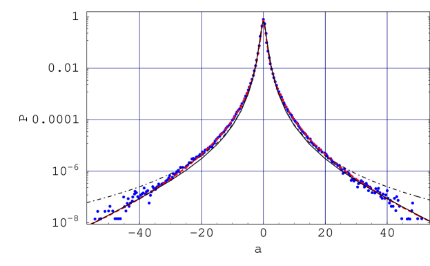
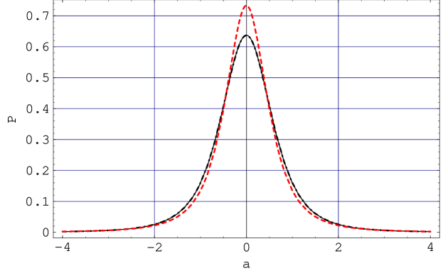
Figure 4: Lagrangian acceleration probability density function $P(a)$. Dots: experimental data for the $R_{\lambda}=690$ flow by Crawford, Mordant, Bodenschatz, and Reynolds.² Dashed line: the stretched exponential fit (4). Dot-dashed line: Beck $\chi$-square model (22), $q=3/2$. Solid line: the $\chi$-square Gaussian model (23), $a_{c}=39.0$, $C=0.637$. $a$ denotes acceleration normalized to unit variance.

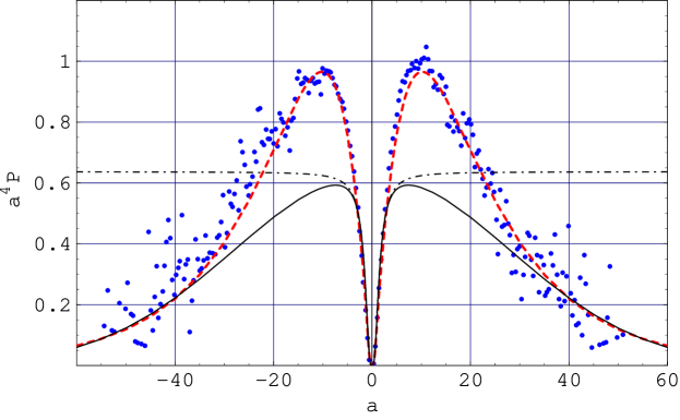
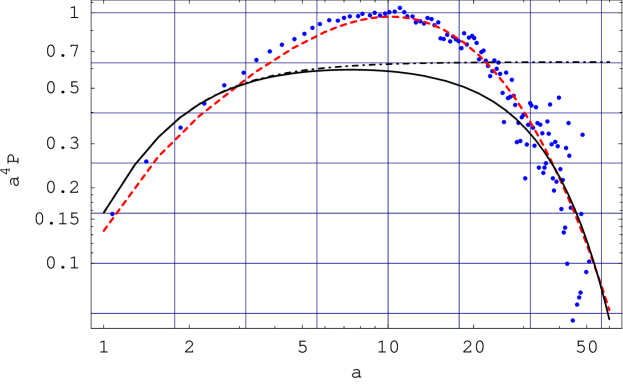
Figure 5: The contribution to fourth-order moment, $a^{4}P(a)$. Top panel: a linear plot, bottom panel: a log-log plot. Same notation as in Fig. 4.

A comparison of the $\chi$-square model (22) and $\chi$-square Gaussian model (23) with the experimental data is shown in Figs. 4 and 5. One can see that both the distributions follow the experimental $P(a)$ to a good accuracy, although the tails of the $\chi$-square model distribution depart from the experimental curve at large $|a|$. A major difference is seen from the contribution to fourth-order moment, $a^{4}P(a)$, shown in Fig. 5. The $\chi$-square model yields a qualitatively unsatisfactory behavior indicating a divergency of the predicted fourth-order moment $\langle a^{4}\rangle$. In contrast, the $\chi$-square Gaussian model is in a good qualitative agreement with the data, reproducing them well at small and large acceleration values although quantitatively it deviates at intermediate acceleration values and gives the flatness value $F\simeq 46.1$ for $a_{c}=39.0$, as compared to the flatness value given by Eq. (5).

3.1.2 The underlying log-normal distribution

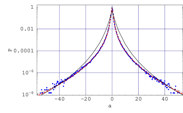
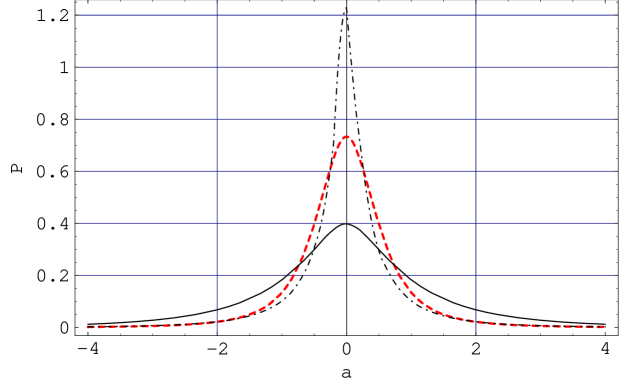
Figure 6: Lagrangian acceleration probability density function $P(a)$. Dots: experimental data for the $R_{\lambda}=690$ flow by Crawford, Mordant, Bodenschatz, and Reynolds.² Dashed line: the stretched exponential fit (4). Dot-dashed line: Beck log-normal model (25), $s=3.0$. Solid line: Castaing log-normal model (26), $s_{0}=0.625$. $a$ denotes acceleration normalized to unit variance.

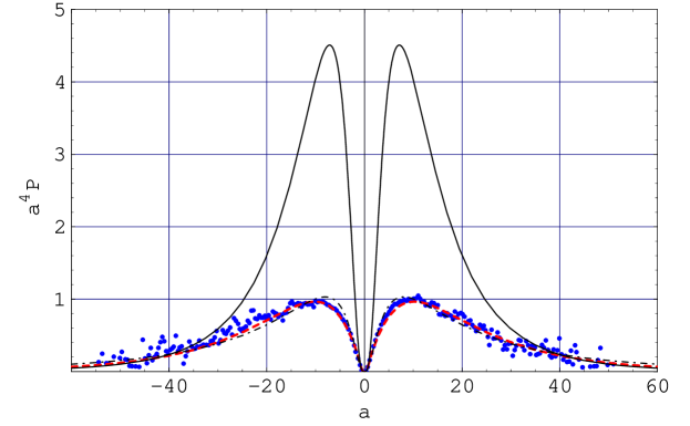
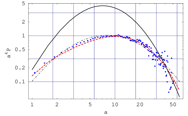
Figure 7: The contribution to fourth-order moment, $a^{4}P(a)$. Top panel: a linear plot, bottom panel: a log-log plot. Same notation as in Fig. 6.

With the log-normal distribution of $\beta$,

$$f(\beta)=\frac{1}{\sqrt{2\pi}s\beta}\exp\left[-\frac{(\ln\frac{\beta}{m})^{2}}{2s^{2}}\right],$$ (24)

the resulting marginal PDF (15) with $P(a|\beta)$ given by the Gaussian (19) was recently proposed to be[34]

$$P(a)=\frac{1}{2\pi s}\int_{0}^{\infty}\!\!\!d\beta\ \beta^{-1/2}\exp\left[-\frac{(\ln\frac{\beta}{m})^{2}}{2s^{2}}\right]e^{-\beta a^{2}/2},$$ (25)

where the only free parameter $s$ can be used for a fitting, or derived from theoretical arguments, $s^{2}=3$ ($m=\exp[s^{2}/2]$ to provide unit variance). This distribution is shown in Fig. 6 and was found to be in a good agreement with the Lagrangian experimental data by La Porta et al.,[1] the new data by Crawford et al.,[2] Mordant et al.,[4] and DNS of the Navier-Stokes equation by Kraichnan and Gotoh.[6]

However, the central part of the distribution shown in Fig. 6 reveals much greater inaccuracy of the log-normal model ($P(0)\simeq 1.23$) as compared with that of both the $\chi$-square and $\chi$-square Gaussian models ($P(0)\simeq 0.65$) which are almost not distinguishable in the region $|a|/\langle a^{2}\rangle^{1/2}\leq 4$ (Fig. 4); see also recent work by Gotoh and Kraichnan.[6] This is the main failing of the log-normal model (25) for $s^{2}=3.0$ although the predicted distribution follows the measured low-probability tails, which are related to acceleration bursts, to a good accuracy. The core of the experimental curve (4) ($P(0)\simeq 0.73$) contains most weight of the experimental distribution and is the most accurate part of it, with the relative uncertainty of about 3% for $|a|/\langle a^{2}\rangle^{1/2}<10$ and more than 40% for $|a|/\langle a^{2}\rangle^{1/2}>40$.[3]

The distribution (25) is characterized by a bit bigger flatness value, $F=3\exp[s^{2}]\simeq 60.3$ for $s^{2}=3$, as compared to the flatness value (5) which is nevertheless acceptable from the experimental point of view. The peaks of the contribution to fourth-order moment shown in Fig. 7 do not match that of the experimental curve for the $R_{\lambda}=690$ flow.

One naturally expects that a better correspondence to the experiment could be achieved by an accounting for small scale interactions via turbulent viscosity [certain nonlinearity in the first term of the rhs of Eq. (16)] as it implies a damping of large events, i.e. less pronounced enhancement of the tails of $P(a)$.

It should be noted that the idea to describe turbulence intermittency via averaging of the Gaussian distribution over lognormally distributed variance of some intermittent variable was proposed long time ago by Castaing, Gagne, and Hopfinger,[63]

$$P(x)=\frac{1}{2\pi s_{0}}\int_{0}^{\infty}\!\!\!d\theta\,\theta^{-2}\exp\left[-\frac{(\ln\frac{\theta}{m_{0}})^{2}}{2s_{0}^{2}}\right]e^{-x^{2}/(2\theta^{2})},$$ (26)

where $x$ is a variable under study. Below, we apply this model to the Lagrangian acceleration, $x=a$.

In technical terms, the difference from the Castaing log-normal model is that in Eq. (25) the inverse square of the variance, $\beta=\theta^{-2}$, is taken to be lognormally distributed. In essence, the models (25) and (26) are of the same type, with different parameters assumed to be fluctuating at large time scale and hence different resulting marginal distributions.

One can check that the change of variable, $\theta=\beta^{-1/2}$, in Eq. (26) leads to the density function different from that given by Eq. (25),

$$P(x)\simeq\int_{0}^{\infty}\!\!\!d\beta\,\beta^{-3/2}\exp\left[-\frac{(\ln\frac{\beta}{m_{1}})^{2}}{2s_{1}^{2}}\right]e^{-\beta x^{2}/2},$$ (27)

where we have denoted $m_{1}=m_{0}^{-2}$ and $s_{1}=2s_{0}$. Therefore, the distributions (25) and (26) are indeed not equivalent to each other, both being of a stretched exponential form.

As to a comparison of the fits, we found that the fit of the Castaing log-normal model (26) for the acceleration, with the fitted value $s_{0}=0.625$ ($m_{0}=\exp[s_{0}^{2}/2]$ for unit variance), is of a considerably lesser quality as one can see from Fig. 6 and, more clearly, from Fig. 7. Positions of the peaks of $a^{4}P(a)$ are approximately the same for both the models, namely, $|a|/\langle a^{2}\rangle^{1/2}\simeq 8.0$ as compared to $|a|/\langle a^{2}\rangle^{1/2}\simeq 10.2$ for the experimental curve.

Notice that the existence and positions of the peaks of $a^{4}P(a)$ reflect some characteristic property of the Lagrangian particle dynamics. The value $|a|/\langle a^{2}\rangle^{1/2}\simeq 10.2$ possibly separates different mechanisms underlying stochastic motion of the particle. One therefore may expect multiple autocorrelation time scales for $a(t)$.

We conclude this subsection with the following remark. The Langevin model of the type (16), Fokker-Planck approximation of the type (18), and the underlying log-normal distribution (24) within the Castaing approach were recently used by Hnat, Chapman, and Rowlands[37] to describe intermittency and scaling of the solar wind bulk plasma parameters. This model will be reviewed in Sec. 3.2 below.

3.1.3 The underlying Gaussian distribution of velocity

The problem of selecting appropriate distribution of the parameter $\beta$ among possible ones was recently addressed in Ref. Aringazin0301245. A specific model based on the assumption that the Lagrangian velocity $u$ follows normal distribution with zero mean and variance $\sigma_{u}^{2}$ was developed. The result is that a class of underlying distributions of $\beta$ can be encoded in the function $\beta=\beta(u)$, and the marginal distribution is found to be

$$P(a)\!=\!C(s)\!\!\int_{0}^{\infty}\!\!\!\!\!\!d\beta\,P(a|\beta)\exp\!\left[{-\frac{[u(\beta)]^{2}}{2\sigma_{u}^{2}}}\right]\!\left|\frac{du}{d\beta}\right|,$$ (28)

where $u(\beta)$ is the inverse function. Note that only an absolute value of $u$ contributes to this probability distribution. Particularly, the exponential dependence

$$\beta(u)=\exp[\pm u],$$ (29)

features the log-normal distribution of $\beta$ so that Eq. (28) leads to Eq. (25) used in Ref. Beck4, while the $\chi$-square distribution of order 1 is recovered when one takes

$$\beta(u)=u^{2}.$$ (30)

In general, this model is relevant when $\beta(u)$ is a monotonic Borel function of the stochastic variable $u$ mapping $(-\infty,\infty)\ni u$ to $[0,\infty)\ni\beta$, and allows one to rule out some ad hoc distributions of $\beta$ as well as to make appropriate generalizations of both $\chi^{2}$ and log-normal distributions of the parameter $\beta$.

The possible dynamical foundation of the above model is as follows. The stationary distribution (28) with $\beta(u)=\exp[\pm u]$ can be associated with the Langevin equation of the form[36]

$$\partial_{t}a=\gamma F(a)+e^{\omega}L(t),$$ (31)

where we denote $\omega=\mp u/2$, $u$ follows Gaussian distribution with zero mean, and we take $\gamma$ = const to simplify the consideration. Here, we adopt a viewpoint that statistical properties of the acceleration $a$ are associated with velocity statistics due to the Heisenberg-Yaglom scaling (6). Notice also that in Sawford model the Langevin equation (1) for $a$ includes velocity $u$ and its variance.

Below, we outline a relationship of the model (31) to some recent approaches in studying the intermittency.

(i) The form of the last term in Eq. (31), in which $\omega$ can be viewed as a Gaussian process $\omega=\omega(t)$ independent of the white noise $L(t)$, strikingly resembles that involved in the recently developed log-infinitely divisible multifractal random walks model by Muzy and Bacry,[49, 50] a continuous extension of discrete cascades.[85] This model will be reviewed in Sec. 6 below.

(ii) The driving force amplitude of the form $e^{\omega(t)}$, with the ultraslow decaying correlation function of $\omega$,

$$\langle\omega(t)\omega(t+\tau)\rangle=-\lambda_{0}^{2}\ln[\tau/T],$$ (32)

$\tau<T$, in the Langevin-type equation has been recently considered by Mordant et al.[4] The results of this model have been found in a very good agreement with the experimentally observed very slow decay of the autocorrelation of Lagrangian velocity increment magnitudes $|\delta_{\tau}u_{i}|$ for each of the two measured component. Also, very slow decay was observed for the cross correlation of magnitudes of components. Both the dynamical correlations were found to vanish only for time scale of about $T_{L}$, while the autocorrelations of full signed $\delta_{\tau}u_{i}$ decay rapidly (the autocorrelation functions cross zero at about $0.06T_{L}$) and the cross correlation function is approximately zero. The used time scale $\tau=0.03T_{L}$. It was emphasized that the parameter $\lambda_{0}$ enters both the model autocorrelation functions of velocity increments and Lagrangian velocity structure functions.

This may correspond to the slow $\bar{\epsilon}/\tau$ decay of the Lagrangian acceleration autocorrelation predicted by K41 theory. We also note that the fitted value of the above intermittency parameter $\lambda_{0}$ ($\lambda_{0}^{2}=0.115\pm 0.01$) is very close to $1/s^{2}=1/3$, with the value $s^{2}=3$ in Eq. (25) interpreted as the number of independent random variables in three-dimensional space at the Kolmogorov scale. If this is not due to a coincidence, the intermittency parameter $\lambda_{0}$ approaches simply the inverse of effective space dimension, $\lambda_{0}=1/d$, $d=3$, for high-Re turbulent flows. The above connection to the MRW model and very slow decay of correlations of absolute values of acceleration components indicate relevance of the specific representation (31), with very slow varying $|u|$, in the description of intermittency. In fact, due to the experiments[29] the Lagrangian velocity autocorrelation function $\langle u(t)u(t+\tau)\rangle/\langle u^{2}\rangle$ decays almost exponentially but very slowly, to vanish only for $\tau>3T_{L}$, where the integral time scale $T_{L}=2.2\times 10^{-2}$ s is two orders of magnitude bigger than the Kolmogorov time scale $\tau_{\eta}=2.0\times 10^{-4}$ s; $R_{\lambda}=740$ and the mean velocity is about 10% of the rms velocity.

(iii) Due to the well-known Kolmogorov power-law relationship between the mean energy dissipation rate $\bar{\epsilon}$ and the rms velocity $\bar{u}$, $\bar{\epsilon}\simeq\bar{u}^{3}/L$, the representation (31) can be thought of as the result of using the relation $\ln\beta\simeq\ln\epsilon$ (statistical law), with $\ln\epsilon$ being normally distributed due to K62 theory.[15] Here, $\epsilon$ denotes stochastic energy dissipation rate per unit mass. From this point of view, one can identify

$$\omega=g\ln\epsilon,$$ (33)

where $g$ is a constant. This means that stochastic dynamics of logarithm of the energy dissipation rate is independent, and it influences the acceleration dynamics specifically through the intensity of driving stochastic force entering Eq. (31). Stationary normal distribution of $\omega$ can be in turn derived from the Fokker-Planck equation associated with the Langevin equation of a linear form, $\partial_{t}\omega=g_{0}+g_{1}\omega+g_{2}L(t)$, where $g_{i}$ are constants. This equation is in an agreement with the recent results of Eulerian (hotwire anemometer) study of the interaction between velocity increments and normalized energy dissipation rate by Renner, Peinke, and Friedrich.[64] Particularly, they found that an exponential dependence of the diffusion coefficient on the logarithmic energy dissipation in the Fokker-Planck equation for the velocity increments in space is in a very good agreement with the experimental data. Notice that this equation does not imply a logarithmic decay of the Lagrangian correlation function $\langle\omega(t)\omega(t+\tau)\rangle$ proposed by Mordant et al.[4] This may be attributed to the well-known difference between the Eulerian (fixed probe) and Lagrangian (trajectory) frameworks.

(iv) For the choice $\beta(u)=\exp[u]$ corresponding to the log-normal distribution of $\beta$, using Eq. (31) one can derive the stationary probability density function of the form[36]

$$P(a)=\int_{-\infty}^{\infty}\!\!du\ C(u)\exp\{\ln[g(u)]-e^{u}a^{2}/2\},$$ (34)

where $g(u)$ is PDF of $u$. Hence the joint PDF can be written

$$P(a,u)=C(u)\exp\{\ln[g(u)]-e^{u}a^{2}/2\}.$$ (35)

Such a form of the distribution, containing specifically the double exponent, resembles the “universal” distribution of fluctuations (Gumbel function),

$$P(x)=c_{0}\exp[c_{1}(y-e^{y})],\quad y\equiv c_{2}(x-c_{3}),$$ (36)

where $c_{i}$ are constant, recently considered by Chapman, Rowlands, and Watkins[68] (see also references therein) following the work by Portelli, Holdsworth, and Pinton[69]. They used an apparently different approach (not related to a Langevin-type equation) based on the multifractal-type energy cascade and $\chi^{2}$ or log-normal (K62 theory) underlying distribution of the energy dissipation rate at fixed level. They pointed out a good agreement of such $P(x)$ with experimental data, where $x$ denotes a fluctuating entity observed in a variety of model correlated systems, such as turbulence, forest fires, and sandpiles. The result of this approach meets ours and we consider it as an alternative way to derive the characteristic probability measure of fluctuations; with $g(u)$ taken to be a $\chi^{2}$ (respectively, Gaussian) density function, one obtains, up to a pre-exponential factor and constants, $P(u)\simeq\exp[-u-\exp(u)]$ (respectively, $P(u)\simeq\exp[-u^{2}-\exp(u)]$). Thus we conclude that the “universal” distribution (36) can be derived also within the general framework proposed in Ref. Aringazin0301245 that reflects a universal character of the underlying $\chi^{2}$ distribution pointed out by Beck and Cohen.[61]

Strong correlation between bursts of Eulerian velocity magnitude and bursts of energy dissipation rate has been indicated in the recent work by Pearson et al.[75] which reports results of DNS of statistically stationary and isotropic slightly compressible $R_{\lambda}\simeq 219$ flow. Unlike to results of some pseudo-spectral methods, highly fluctuating character of time series of $\epsilon$, $L$, $u$, and $R_{\lambda}$, where $L$ and $u$ are characteristic large length and velocity scales respectively, has been encountered. A correct procedure for determination of $R_{\lambda}$ dependence of $C_{\epsilon}=\bar{\epsilon}L/{\bar{u}}^{3}$ is based on accounting for time lapse between the bursts and for the averaging over entire time series for which stationarity condition is fulfilled. This leads to elimination of the scatter in determining the value of $C_{\epsilon}$ from various recent DNS and experimental data. The value $C_{\epsilon}\simeq 0.5$ has been established as the high-Re asymptotic value, which is in agreement with K41 assumption on viscosity independence of the mean turbulent kinetic energy dissipation rate for stationary isotropic turbulence.

In summary, we have presented a class of models (28)-(31) using the basic assumption that the parameter $\beta$ depends on normally distributed velocity fluctuations. This class has been found to incorporate the previous RIN models in a unified way, with the dependence $\beta(u)$ required to be a (monotonic) Borel function of the stochastic variable $u$.

Finally, we note that although successful in describing the observed statistics of Lagrangian acceleration, with a few simple hypotheses and one fitting parameter, the one-dimensional Langevin RIN models (15)-(18) and (28)-(31) show departures from the experimental data and suffer from the lack of physical interpretation in the context of the 3D Navier-Stokes turbulence.

3.2 Hnat-Chapman-Rowlands model

A nonlinear Langevin and the associated Fokker-Planck equations obtained by a direct requirement that the probability distribution satisfies some model-independent scaling relation have been recently proposed by Hnat, Chapman, and Rowlands,[37] to describe the measured time series of the solar wind bulk plasma parameters. It should be emphasized that this approach is related to properties of Fokker-Planck equation rather than to those of Langevin-type equation. Nevertheless, we find this result relevant to fluid turbulence since it is based on a stochastic dynamical framework and leads to the stationary distribution with exponentially truncated power-law tails, similar to that implied by the RIN models of Sec. 3.1.

The Hnat-Chapman-Rowlands model is aimed to describe the observed time series of the solar wind bulk plasma parameters and is based on the construction of Fokker-Planck equation for which the probability density function obeys the following one-parametric model-independent rescaling:

$$P(x,t)=t^{-\alpha_{0}}P_{s}(xt^{-\alpha_{0}}).$$ (37)

Here, $x$ denotes fluctuating plasma parameter and $\alpha_{0}$ is the scaling index. Particularly, the value $\alpha_{0}=1/2$ corresponds to a self-similar (Brownian) walk with Gaussian probability density functions at all time scales. The fitted value is different, $\alpha_{0}=0.41$, and corresponds to a single non-Gaussian distribution $P_{s}(x_{s})$, to which the observed distributions of some four plasma parameters collapse under the scaling $x_{s}=xt^{-\alpha_{0}}$.

The Langevin equation of this model assumes only additive noise, and in such ansatz it was found to be

$$\partial_{t}x=D_{1}(x)+D_{2}(x)\eta(t),$$ (38)

where $D_{1}$ and $D_{2}$ are of the form

$$D_{1}(x)=\sqrt{\frac{b_{0}}{D_{0}}}x^{1-\alpha_{0}^{-1}/2},$$ (39)

$$D_{2}(x)=[b_{0}(1-\alpha_{0}^{-1}/2)-a_{0}]x^{1-\alpha_{0}^{-1}},$$ (40)

$a_{0}$ and $b_{0}$ are free parameters and $2D_{0}$ is intensity of the $\delta$-correlated Gaussian-white additive noise $\eta(t)$, $\langle\eta(t)\rangle=0$. By construction, this specific form of the dynamical equation ensures that the corresponding Fokker-Planck equation

$$\partial_{t}P(x,t)=\partial_{x}[a_{0}x^{1-\alpha_{0}^{-1}}P+b_{0}x^{2-\alpha_{0}^{-1}}\partial_{x}P]$$ (41)

has the general solution $P(x,t)$, which exhibits the scaling (37). The fitted values are $a_{0}/b_{0}=2$, $b_{0}=10$, and $\alpha_{0}^{-1}=2.44$. The rescaled distribution $P_{s}(x_{s})$ corresponding to Eq. (41) is characterized by power-law tails truncated by stretched exponential. It provides a good fit to the tails of the experimental distribution but diverges at the origin $x_{s}\to 0$.

To sum up, we point out that this diffusion model uses the generalized self-similarity principle resembling that used in the Eulerian description of the energy cascade in the developed 3D fluid turbulence and appears to be valid only asymptotically for large values of the variable, with the fitted value of exponent parameter being about $\alpha_{0}=0.41$.

3.3 Reynolds stochastic models of Lagrangian acceleration

The second-order Lagrangian stochastic model of Reynolds[38, 39] which extends Sawford model (1) is prescribed by the following equation for a component of acceleration:

$$da=-(T_{L}^{-1}\!+\!\tau_{\eta}^{-1}\!-\!\sigma_{a|\epsilon}^{-1}\frac{d\sigma_{a|\epsilon}}{dt})adt\!-\!T_{L}^{-1}\tau_{\eta}^{-1}udt\!+\!\sqrt{2\sigma_{u}^{2}(T_{L}^{-1}\!+\!\tau_{\eta}^{-1})T_{L}^{-1}\tau_{\eta}^{-1}}d\xi.$$ (42)

Here, $d\xi$ is an incremental Wiener process with zero mean and variance $dt$, the energy-containing and dissipative time scales of flow $T_{L}=2\sigma_{u}^{2}/(C_{0}\epsilon)$ and $\tau_{\eta}=C_{0}\nu^{1/2}/(2a_{0}\epsilon^{1/2})$ are defined in terms of the stochastic dissipation rate $\epsilon$, universal Lagrangian structure constants $a_{0}$ and $C_{0}$, the kinematic viscosity $\nu$, and the velocity variance $\sigma_{u}^{2}\equiv\langle u^{2}\rangle\equiv{\bar{u}}^{2}$.

Model prediction for the Lagrangian acceleration PDF is due to $P(a)=\int_{0}^{\infty}P(a|\epsilon)f(\epsilon)d\epsilon$, where one assumes independent zero-mean Gaussian distributions for velocity and acceleration with variances $\sigma_{u}^{2}$ and $\sigma_{a|\epsilon}^{2}$ respectively. This model is featured by accounting for fluctuations of $\epsilon$ and is consistent with the log-normal model reviewed in Sec. 3.1.2.

In order to calculate $P(a)$ one should determine distribution of the turbulent energy dissipation rate $\epsilon$. Following Pope and Chen,[70] the evolution of logarithm of the normalized dissipation rate $\chi=\ln(\epsilon/{\bar{\epsilon}})$ along a Lagrangian trajectory is governed by the stochastic equation

$$d\chi=-(\chi-\langle\chi\rangle)T_{\chi}^{-1}dt+\sqrt{2\sigma_{\chi}^{2}T_{\chi}^{-1}}d\xi^{\prime},$$ (43)

where $d\xi^{\prime}$ is independent incremental Wiener process with zero mean and the time scale $T_{\chi}=2\sigma_{u}^{2}/C_{0}\langle\chi\rangle$. The distribution of $\chi$ is thus Gaussian, and its variance was approximated by $\sigma_{\chi}^{2}=0.354+0.289\ln R_{\lambda}$, in accordance with K62 theory and DNS data by Yeung and Pope.[71] Thus, Reynolds-number effects are incorporated into the model, which is applicable to large time scale. It should be emphasized that the introduction of fluctuating $\chi$ means that the model (42) incorporates both additive and multiplicative noises.

The resulting acceleration flatness factor behaves as $F=1.35R_{\lambda}^{\,0.65}$, which is in agreement with the recent pressure gradient DNS data by Kraichnan and Gotoh[6] and with lower bound on $F$ set by the experiment.[1] The obtained PDF $P(a)$ is in agreement with the measured acceleration distribution.[1, 2] Also, the model agrees well with the observed extended self-similarity of the Lagrangian velocity structure functions, the exponential shape of the Lagrangian velocity autocorrelation functions, and the observed ultraslow correlation of the modulus of the acceleration[4, 29] (see Sec. 3.1.3).

Extension of this model to account for the observed dependence of the acceleration variance on velocity[40] will be reviewed in Sec. 5 below.

One of the important dynamical quantities of a fluid particle motion are trajectory rotations. Recently developed second-order 3D model by Reynolds and Veneziani[43] shows that non-zero mean trajectory-rotations are associated with spiralling trajectories, oscillatory Lagrangian velocity autocorrelation functions, suppressed rates of turbulent dispersion for given turbulent kinetic energy and mean dissipation rate, and skew diffusion; see also work by Borgas, Flesch, and Sawford.[72] The 3D stochastic model equation includes terms of the form $\epsilon_{ijk}\Omega_{j}u_{k}dt$, and the resulting stationary joint PDF

$$P(a,u)=(2\pi\sigma_{a}^{2}\sigma_{u}^{2})^{-3}\exp\left[\frac{(a_{i}-\epsilon_{ijk}\Omega_{j}u_{k})^{2}}{2\sigma_{a}^{2}}\right]\exp\left[\frac{u_{i}^{2}}{2\sigma_{u}^{2}}\right]$$ (44)

is of a Gaussian form with respect to $a_{i}$ and $u_{i}$. Here, $\sigma_{a}^{2}=\sigma_{u}^{2}/(T_{L}\tau_{\eta})$ is the conditional acceleration variance. The conditional mean acceleration $\langle a_{i}|u\rangle=\epsilon_{ijk}\Omega_{j}u_{k}$ entering the distribution (44) endows trajectories with a preferred sense of rotation.

They showed that rotations of the Lagrangian velocity vector produced by such model coincide closely with the intense rotations measured in the recent seminal experiment by Zeff et al.[73] and are described by Tsallis statistics[32, 60, 61] to a good accuracy. Model predictions for the rotational statistics of the North Atlantic Ocean are found to be in close agreement with simulation data produced by the Miami Isopycnic-Coordinate Ocean Model.

In a recent paper Reynolds[41] constructed phenomenological third-order Lagrangian stochastic model. The model describes evolution of the material derivative of acceleration, the so called hyper-acceleration ${\dot{a}}=da/dt$, in analogy with the second-order model. The 1D stochastic equation for ${\dot{a}}$ is

$$d{\dot{a}}=-(T_{L}^{-1}\!+\!\tau_{\eta}^{-1}+t_{3}^{-1}){\dot{a}}dt-(T_{L}^{-1}\tau_{\eta}^{-1}\!+\!T_{L}^{-1}t_{3}^{-1}+\tau_{\eta}^{-1}t_{3}^{-1})adt$$

$$-T_{L}^{-1}\tau_{\eta}^{-1}t_{3}^{-1}udt+\sqrt{2\sigma_{{\dot{a}}|a\,u}^{2}(T_{L}^{-1}\!+\!\tau_{\eta}^{-1}+t_{3}^{-1})}d\xi,$$ (45)

$da={\dot{a}}dt$, $du=adt$, two timescales $T_{L}$ and $\tau_{\eta}$ are defined as above, and $t_{3}$ is third timescale related to the hypothesis of finite hyper-acceleration variance. The hyper-acceleration is assumed to be autocorrelated exponentially on the timescale $t_{3}\ll\tau_{\eta}$, in a fully developed turbulent flow. The hyper-acceleration variance $\sigma_{{\dot{a}}|a\,u}^{2}=\sigma_{\dot{a}}^{2}-\sigma_{a}^{4}/\sigma_{u}^{2}$ is taken conditional on both the acceleration $a$ and velocity $u$ through their variances.

As in the case of the second-order model, this model applies to stationary homogeneous and isotropic turbulence with Gaussian velocity and acceleration statistics. The hyper-acceleration statistics is Gaussian. The 1D toy model given by Eq. (3.3) is determined uniquely by the well-mixed condition. The corresponding Lagrangian velocity autocorrelation function is consistent with the inertial range and dissipation range forms of Lagrangian velocity structure functions by Kolmogorov similarity theory.

The model timescales are related to the variances of velocity, acceleration, and hyper-acceleration by

$$\sigma_{a}^{2}=\sigma_{u}^{2}(T_{L}\tau_{\eta}+T_{L}t_{3}+\tau_{\eta}t_{3})^{-1},\quad\sigma_{\dot{a}}^{2}=\sigma_{a}^{2}(T_{L}^{-1}\tau_{\eta}^{-1}\!+\!T_{L}^{-1}t_{3}^{-1}+\tau_{\eta}^{-1}t_{3}^{-1}).$$ (46)

For $t_{3}=0$ it follows particularly that $\sigma_{a}^{2}=\sigma_{u}^{2}/(T_{L}\tau_{\eta})=a_{0}{\bar{\epsilon}}^{3/2}\nu^{-1/2}$ in an agreement with Heisenberg-Yaglom scaling law (non-intermittent K41 picture) given by Eq. (6); ${\bar{\epsilon}}={\bar{u}}^{3}/L$ and $a_{0}$ is constant.

In fact, the third-order model goes beyond Kolmogorov phenomenological theory by introducing third characteristic time-scale $t_{3}$, in addition to the conventional time scales $T_{L}$ (energy-containing) and $\tau_{\eta}$ (dissipative). For $t_{3}\not=0$ one thus expects deviations from the K41 predictions. Particularly, corrections due to intermittency are known to imply dependence of the Kolmogorov constant $a_{0}$ on Reynolds number. While for high-Re flows $a_{0}$ is found approximately constant (however, weak deviations such as $a_{0}\simeq R_{\lambda}^{0.14}$ can not be ruled out), for $R_{\lambda}<500$ there is a clear deviation from the K41 scaling of the acceleration variance.[1]

Agreement between third-order model predictions and DNS data for Lagrangian velocity structure function and Lagrangian acceleration autocorrelation function is found significantly better than that obtained with the second-order Lagrangian stochastic model (42). The effects of third-order processes were found comparable in magnitude to the effects of second-order processes.

This means that the third-order dynamics at the characteristic time scale $t_{3}$ is essential for a better description of homogeneous isotropic turbulence within the framework of such a Lagrangian stochastic modeling approach. Physical interpretation of such (and higher-order) processes in the context of 3D Navier-Stokes equation and turbulence phenomenology is one of the open problems.

Anisotropy effects in turbulence within the framework of Lagrangian stochastic third-order model has been described by Reynolds, Yeo, and Lee.[42] The simplest 3D stochastic equation for the hyper-acceleration in homogeneous anisotropic turbulence is given by

$$d{\dot{a}}_{i}=(a_{ij}+c_{ij}){\dot{a}}_{j}dt+(b_{ij}-c_{ik}a_{kj})a_{j}dt+c_{ik}b_{kj}u_{j}dt+\sqrt{-2(a_{ij}+c_{ij})\lambda_{jk}}d\xi_{k},$$ (47)

with $da_{i}={\dot{a}}_{i}dt$ and $du_{i}=a_{i}dt$. Here, $a_{ij}=-C_{0}\epsilon\tau_{ij}-2a_{0}C_{0}^{-1}(\epsilon/\nu)^{1/2}\delta_{ij}$, $b_{ij}=-a_{0}(\epsilon^{3}/\nu)^{1/2}\tau_{ij}$, $c_{ij}(\chi_{jk}+b_{jl}\sigma_{lk})=-a_{ij}\chi_{jk}$, $\tau_{ij}=[\sigma^{-1}]_{ij}$, and $\sigma_{ij}=\langle u_{i}u_{j}\rangle$, $\chi_{ij}=\langle a_{i}a_{j}\rangle$, and $\lambda_{ij}=\langle{\dot{a}}_{i}{\dot{a}}_{j}\rangle$ are Lagrangian velocity, acceleration, and hyper-acceleration covariances respectively; $i,j,\dots=1,2,3$ (summation over repeated indices is assumed). When the inverse time scales $c_{ij}$ of third-order processes tends to infinity the model (47) reduces to a second-order Lagrangian stochastic model.

Model predictions were compared with the results of DNS acquired for a turbulent channel flow with low Reynolds number $R_{\lambda}\simeq 30$. The third-order model is shown to account naturally for the anisotropy of acceleration variances in low-Re turbulent flows and for their dependency upon the energy-containing scales of motion. The experimental values $C_{0}=6.0$ and $a_{0}=5.5$ were taken and the hyper-acceleration variances were subsequently chosen to guarantee consistency with the DNS data for the acceleration variances.

As to the high-Re limit, it was argued that if $t_{3}/\tau_{\eta}$ tends to a finite value when $R_{\lambda}\to\infty$ then hyper-acceleration statistics may account for the observed anisotropy of acceleration variances in high-Re flows.[1] Alternatively, if $t_{3}/\tau_{\eta}\to 0$ for $R_{\lambda}\to\infty$ then one ends up with the isotropic scaling prediction. It was argued that $t_{3}\not=0$ implies in general dependence of the acceleration on the energy-containing scales of motion through the dependence of Lagrangian acceleration variance $\sigma_{a}^{2}$ upon $\sigma_{u}^{2}$ for each component separately.

Non-universality of parameters in conventional Lagrangian stochastic models, when one tries to fit them to experimental and DNS data, was shown to be a consequence of truncation at either first or second order and not an inherent deficiency of the approach in general. Anisotropy of acceleration variance implies “anisotropy” of $a_{0}$ (different values of $a_{0}$ for different components) when $t_{3}=0$. This is not necessarily the case for $t_{3}\not=0$. The additional dynamical degree of freedom provided by the third-order model, i.e. inclusion of third-order processes to describe homogeneous turbulence, thus allows one to keep universal character of some parameters when fitting model predictions to the experiments and DNS.

3.4 Laval-Dubrulle-Nazarenko model of small-scale turbulence

The above one-dimensional Langevin toy models of Lagrangian turbulence considered in Secs. 3.1, 3.2, and 3.3 all suffer from the lack of physical interpretation, e.g. of short-term dynamics, or small- and large-scale contributions, in the context of 3D Navier-Stokes equation.

The crucial point is to make a link between Langevin-type equations and the 3D Navier-Stokes equation. This includes determination of statistical properties of stochastic terms and the functional form of deterministic terms, as well as their dependence on the parameters entering the Navier-Stokes equation, justified for fully developed turbulence. Also, some extension of the stochastic equation may be required to account for dependence of the parameters on Lagrangian velocity, in the spirit of RIN approach of Sec. 3.1, and in correspondence to the Navier-Stokes equation as the pressure gradient term in the Eulerian framework can be expressed in terms of the velocity owing to the incompressibility condition. Strong and nonlocal character of Lagrangian particle coupling as the result of pressure effects makes it difficult to derive theoretically turbulence statistics from the 3D Navier-Stokes equation. One is thus left with more or less justified modeling approaches.

The Navier-Stokes equation based approach to describe statistical properties of small scale velocity increments, both in the Eulerian and Lagrangian frameworks, was developed in much detail by Laval, Dubrulle, and Nazarenko;[44] see also recent paper by Laval, Dubrulle, and McWilliams.[45]

This approach is based on featuring nonlocal interactions between well separated large and small scales —elongated triads— and is referred to as the Rapid Distortion Theory (RDT) approach. Decomposition of velocities into large- and small-scale parts was made by introducing a certain spatial filter of a cutoff type. Within the framework of this approach, 3D Langevin-type model of small-scale turbulence was proposed.

The main assumption of the Laval-Dubrulle-Nazarenko (LDN) approach to the 3D Navier-Stokes turbulence is to introduce and separate large-scale ($L$) and small-scale ($l$) parts in the 3D Navier-Stokes equation and using the Gabor transform (Fourier transform in windows)[44, 74]

$${\hat{u}}_{i}(x_{n},k_{m},t)=\int f(\varepsilon|x_{j}-x^{\prime}_{j}|)e^{ik_{m}(x_{m}-x^{\prime}_{m})}u_{i}(x^{\prime}_{n},t)\mathrm{d}^{3}x^{\prime}_{s}.$$ (48)

Here, the parameter $\varepsilon$ is such that $2\pi/L\ll\varepsilon\ll 1$ and $f(x)$ is a function which decreases rapidly in infinity. The “window” to which Fourier transform applies is centered at the point $x_{m}$ and has the size between small and large scales $l$ and $L$ respectively.

This allows to consider analytically small-scale turbulence coupled to large-scale terms, i.e. account for an inter-scale coupling. Such nonlocal interactions were argued to be important in understanding intermittency in developed turbulent flows. The other, large-scale, part of the equation can be treated separately (and, in principle, solved numerically given the forcing and boundary conditions) since the forcing is characterized by presumably narrow range of small wave numbers, and the small scales make little effect on it. Small-scale interactions are modeled by a turbulent viscosity and were shown numerically to make small contribution to the anomalous scaling (intermittency) in the decaying turbulence. Nevertheless, these are important when fitting model distribution to the experimental data. The 3D LDN model of small scale turbulence was used to formulate surrogate 1D LDN model, which was studied both in the Eulerian and Lagrangian frames.[44]

The 1D LDN toy model of the Lagrangian turbulence implies a nonlinear Langevin-type equation for a component of small-scale velocity increments in time.[44] Such a toy model can also be viewed as a passive scalar in a compressible 1D flow. For sufficiently small time scale $\tau$ it corresponds to the acceleration $a$ of fluid particle, $a=\delta_{\tau}u/\tau$, and is written as[46, 48]

$$\partial_{t}a=(\xi-\nu_{\mathrm{t}}k^{2})a+\sigma_{\perp}.$$ (49)

This equation corresponds to a Lagrangian description in the scale space, along a wave-number packet, defined by the Gabor transform. Here,

$$\nu_{\mathrm{t}}=\sqrt{\nu_{0}^{2}+B^{2}a^{2}/k^{2}}$$ (50)

stands for the turbulent viscosity introduced to describe small-scale interactions, $\nu_{0}$ is the kinematic viscosity, $B$ is a free parameter, $k$ is the wave number [$\partial_{t}k=-k\xi$, $k(0)=k_{0}$, to model the RDT stretching effect in 1D case], $\xi$ and $\sigma_{\perp}$ are multiplicative and additive noises associated with the velocity derivative tensor and forcing of small scales by large scales (the energy transfer from large to small scales), respectively. We refer to the model (49) as the 1D LDN-type model of Lagrangian acceleration in turbulence.

The entities $\sigma_{\perp}$ and $\xi$ in Eq. (49) are surrogate versions of the 3D entities related to large- and small-scale parts $U_{i}$ and $u_{i}$ of the velocity field as follows:[44]

$$\hat{\bm\xi}=\bm\nabla\left[\frac{2\bm{k}}{{\bm k}^{2}}(\bm{k}\cdot\bm{U})-\bm{U}\right],$$ (51)

$$\hat{\bm\sigma}_{\perp}=\hat{\bm\sigma}-\frac{\bm k}{{\bm k}^{2}}(\bm{k}\cdot\hat{\bm\sigma}),$$ (52)

$$\sigma_{i}=\partial_{j}(\overline{U_{i}U_{j}}-U_{i}U_{j}+\overline{u_{j}U_{i}}-\overline{U_{j}u_{i}}),$$ (53)

where the hat denotes Gabor transform (48) and the overline stands for certain spatial cutoff retaining a large-scale part. Statistical properties of all the components of ${\bm\xi}$ and ${\bm\sigma}_{\perp}$ were studied numerically for decaying turbulence and reveal rich and complex behavior.

One can see from Eqs. (51)-(53) that the noises are related to the velocities and their derivatives, and the additive noise $\bm\sigma_{\perp}$ is associated with interaction terms between the large- and small-scale dynamics. One therefore expects that this noise may exhibit both the short- and long-time autocorrelations. Physically, this would correspond to vortical structures dynamics of which is essentially characterized by two well separated time scales.

This gives support to the idea that the intermittency is caused also by some nonlocal interactions including the inertial-range flow modes and not merely by small scales. We remark that one would also like to know the role of the dissipative scale in this integrated picture.[23]

Noisy character of the entities (51) and (52) may not be seen as a consequence of the Navier-Stokes equation, which does not contain external random forces at the characteristic time scale. In the RDT approach, $\xi$ and $\sigma_{\perp}$ are treated as independent stochastic processes entering the small-scale dynamics (49) owing to the fact that the large-scale dynamics is weakly affected by small scales (which corresponds to a direct energy cascade in 3D flow) and thus can be viewed, in the first approximation, as a given force of a stochastic character with certain ascribed autocorrelation along a particle trajectory.

Eqs. (49) and (51)-(53) could be used to trace back the origin of multiplicative and additive noises entering various surrogate Langevin-type models of the developed turbulence, and to provide important information on the dynamics underlying the intermittency.

As a first step, in 1D case these noises were modeled in the Lagrangian frame by coupled Gaussian-white noises[44] inspired by the Kraichnan ensemble used for turbulent passive scalar and the Kazantsev-Kraichnan model of turbulent dynamo,

$$\langle\xi(t)\rangle=0,\ \langle\xi(t)\xi(t^{\prime})\rangle=2D\delta(t-t^{\prime}),$$

$$\langle\sigma_{\perp}(t)\rangle=0,\ \langle\sigma_{\perp}(t)\sigma_{\perp}(t^{\prime})\rangle=2\alpha\delta(t-t^{\prime}),$$ (54)

$$\langle\xi(t)\sigma_{\perp}(t^{\prime})\rangle=2\lambda\delta(t-t^{\prime}),$$

where $D$, $\alpha$, and $\lambda$ are free parameters depending on scale via $k_{0}$. The positive parameters $D$ and $\alpha$ measure intensities of the multiplicative and additive noises respectively, while $\lambda$ (to be not confused with the Taylor microscale) measures correlation between the noises.

The representation (3.4) puts an obvious limitation but is partially justified by DNS.[44] The averaging in Eq. (3.4) is made over ensemble realizations. Zero means correspond to isotropy of the stochastic forces along a trajectory. Physically, the small scales are thus assumed to be essentially distorted in a stochastic way, as a combined effect of much larger scales. The model (3.4) accounts for short-time autocorrelations (approximated by zero-time autocorrelations), with the parameters $D$, $\alpha$, and $\lambda$ treated here as constants along a particle trajectory.

We stress that the correlation between the noises $\xi$ and $\sigma_{\perp}$ defined by Eq. (3.4) is not ad hoc assumption but a consequence of the structure of their 3D counterparts (51) and (52) as they contain the same large-scale velocity serving as a unifying agent between the noises.

Partial support of the argument that large scales influence much smaller scales is due to the recent study by Pearson et al.[75] of the so called “zeroth law” of turbulence. Comparing Lumley’s forward cascade model prediction and DNS data they argue that some amount of energy is passed to all higher wave numbers, not totally to the neighboring wave numbers, at least for low $R_{\lambda}\sim O(10^{2})$. Whether this holds for higher-Re flows is however still an open question.

Stationary solution of the Fokker-Planck equation associated with Eq. (49) and the noises (3.4),

$$\partial_{t}P(a,t)=\partial_{a}(\nu_{\mathrm{t}}k^{2}P)+D\partial_{a}(a\partial_{a}aP)-\lambda\partial_{a}(a\partial_{a}P)-\lambda\partial^{2}_{a}(aP)+\alpha\partial^{2}_{a}P,\$$ (55)

is given by[44]

$$P(a)=C\exp\left[\int_{0}^{a}dy\frac{-\nu_{\mathrm{t}}k^{2}y-Dy+\lambda}{Dy^{2}-2\lambda y+\alpha}\right],$$ (56)

where $C$ is a normalization constant and six parameters can be used to fit the experimental data. This model specifies the one-dimensional LDN model (49), and we refer to this model as the LDN model with $\delta$-correlated noises (dLDN model).

Thus, one makes a closure by treating the combined effect of large scales, for which one has a different dynamical LDN equation that could be in principle solved numerically,[76] and nonlocal inter-scale coupling as a pair of given external noises. The price of the simplification (3.4) is that one introduces free parameters $\alpha$, $D$, and $\lambda$ to the description. Matching large-scale dynamics to boundary conditions deserves a separate study. Despite 3D turbulence is known to be more sensitive to the large-scale forcing or boundary conditions, as compared to the 2D one, the used simplification (3.4) is relevant for high-Re flows to some extent[44, 76] and allows one to advance in analytical treatment of the problem.

It should be stressed that the 1D LDN toy model (49) as well as its particular case, dLDN model, have several limitations related to the LDN separation of small and large scales allowing to study exclusively nonlocal effects associated with the linear process of distortions of small scales by a strain produced by large scales; the use of model turbulent viscosity; and one-dimensionality. Applicability of the model at Lagrangian integral time scale is limited due to the used separation of scales. Formulation of the model to include description at the integral time scale in a consistent way is of much interest. Our remark is that one of the possible formal ways to account for Reynolds-number effects is to assume that intensities of the external noises, which represent large scales, depend on Reynolds number.

Langevin-type equation containing both the Gaussian-white multiplicative and additive noises was studied in detail by Nakao.[77] The associated Fokker-Planck equation was also analyzed. The dLDN model (49) extends Nakao’s set up by incorporating two new features: (i) the nonlinearity controlled by $B$ in Eq. (50) and (ii) the coupling of the noises controlled by $\lambda$ in Eq. (3.4).

It is interesting to note that the RDT approach qualitatively resembles the model studied by Kuramoto and Nakao,[78] a system of spatially distributed chaotic elements driven by a field produced by nonlocal coupling, which is spatially long-wave and temporally irregular. Such systems, in which the multiplicative noise is the local Lyapunov exponent fluctuating randomly due to the chaotic motion of the elements, show power-law correlations, intermittency, and structure functions similar to that of the developed fluid turbulence.

Finally, we note that different strategy to obtain single-particle PDF of Lagrangian velocity increments from the 3D Navier-Stokes equation, without referring to Langevin-type equations, is due to the Lagrangian PDF method[24] outlined in Introduction.

Before turning to a comparison of the LDN and RIN models which will be made in Sec. 4 below, it is worthwhile to outline recent results on RDT approach to small-scale turbulence.

Within the framework of RDT approach, new physical measures of intermittency such as the mean polarization and the spectral flatness have been introduced recently by Dubrulle, Laval, Nazarenko, and Zaboronski[76] by using the Gabor transform of separated large- and small-scale velocities and a method previously developed for the kinematic dynamo problem.[79] The resulting equation for the small-scale Gabor transformed velocity ${\hat{u}}_{m}={\hat{u}}_{m}(k,x(t),t)$, for the fluid-particle trajectory determined by $\partial_{t}x_{i}(t)=U_{i}$, has been found in the following form:

$$\partial_{t}{\hat{u}}_{m}=\sigma_{ij}k_{i}\frac{\partial{\hat{u}}_{m}}{\partial k_{j}}-\sigma_{mi}{\hat{u}}_{i}+\frac{2}{k^{2}}k_{m}\sigma_{ij}k_{i}{\hat{u}}_{j}-\nu k^{2}{\hat{u}}_{m},$$ (57)

where $\sigma_{ij}(t)=\nabla_{j}U_{i}$ is the large-scale strain. The nonlinear advection term entering the 3D Navier-Stokes equation has been neglected. Hence local interactions among small scales are not considered. Nevertheless, Eq. (57) is of much interest since one can investigate contribution of nonlocal interactions.

Gaussian white-noise processes for large-scale strain matrix components (rapid stochastic distortions of small scales), the form of which ensures statistical isotropy near a fluid-particle path and the incompressibility,

$$\langle\sigma_{ij}(\tau)\sigma_{kl}(0)\rangle=\Omega(\delta_{ik}\delta_{jl}-d^{-1}\delta_{ij}\delta_{kl})\delta(\tau),$$ (58)

have been taken as a model representation; $i,j,\dots=1,2,\dots,d$. This representation in Eq. (57) was used to derive time-evolution equation for the generating function

$$Z(k,t)=\langle\exp[\lambda_{1}|{\hat{u}}_{m}|^{2}+\lambda_{2}{\hat{u}}_{m}^{2}+\lambda_{3}{\hat{u}}_{m}^{*2}]\rangle,$$ (59)

where $\lambda_{1,2,3}$ are auxiliary parameters, $\Omega$ is constant, and $d=3$ for three dimensions. Due to the isotropy the final equation depends only on the module of wave number, $k=|\bm k|$. The model (57)-(58) is referred to as Stochastic Distortion Theory (SDT) model.

From the equation for $Z$ an evolution equation for the Gabor-velocity correlators of even order can be extracted in a standard way. Inviscid regime and dissipative regime approximations of the obtained correlators have been presented.

Fourth-order wave-number space correlators are shown to carry essential information on the turbulence statistics and intermittency which is not available from the two-point spatial correlators widely used in studying turbulence. Particularly, the mean polarization carries information on amplitudes and phase difference of Gabor modes. All turbulence wavepackets are shown eventually to become plane polarized, $\langle|{\hat{u}}_{i}|^{4}\rangle\simeq\langle|{\hat{u}}_{i}^{2}|^{2}\rangle$, i.e. the turbulence tends to be strongly non-Gaussian. Also, the spectral flatness, in the inviscid regime, increases as $k^{3/2}$ with the increase of wave number $k$ that indicates presence of small-scale intermittency. The effects of dissipation have been quantified.

It was also argued that the log-normal character of turbulence statistics (nonlinearity in the order of correlator appears to be of a square form in the exponent) arises because the strain in SDT model is a multiplicative noise for the velocity, which becomes nearly one-dimensional, and the time integrated strain tends to become a Gaussian process.

We note that the used model statistics of strain (58) is characterized by $\delta$-correlations and does not contain long-time fluctuating terms. Such fluctuations could be accounted for by taking, for example, $\Omega$ to be long-time correlated stochastic process, which corresponds to a slow-varying random intensity of the noisy strain along a particle trajectory.

In the following Section, we make a comparison of the RIN model (15)-(18) with the LDN-type model (49), as well as its particular case, the dLDN model (56).[46]

4 Comparison of the simple RIN and LDN-type models

4.1 A qualitative comparison

A direct comparison of the Langevin equations (16) and (49) of the two models suggests the following evident identifications:

$$\gamma F(a)=(\xi-\nu_{\mathrm{t}}k^{2})a,\quad\sigma L=\sigma_{\perp}.$$ (60)

Hence the additive noises can be made identical to each other by putting $\sigma^{2}=\alpha$. Further, in the case of a linear drift force, $F(a)=-a$, and constant viscosity, $\nu_{\mathrm{t}}=\nu_{0}$, we can identify the remaining parameters, $\gamma=\nu_{0}k^{2}-\xi$, so that we get

$$\beta\equiv\gamma/\sigma^{2}=(\nu_{0}k^{2}-\xi)/\alpha.$$ (61)

This relation implies that the parameter $\beta$ can be viewed as a stochastic variable with a nonzero mean due to the stochastic nature of $\xi$ assumed in the LDN model. This is in agreement with the simple RIN model, the defining feature of which is just that the fluctuating part of $\beta$ follows some statistical distribution. Such a general procedure for obtaining Tsallis-type statistics was suggested in Ref. Aringazin0204359.

In the dLDN model (49)-(56), both the additive and multiplicative noises are taken $\delta$-correlated due to Eq. (3.4). This is in a sharp contrast to the assumption that $\beta$ can be taken constant to derive the stationary solution (19) which is the foundation of the simple RIN model. More precisely, the solution in the form (19) can be obtained as the lowest-order approximation if $\beta$ is slow varying in time as compared to a typical time scale associated with the additive noise $L(t)$ (the adiabatic approximation). This suggests that the multiplicative noise $\xi$ should be taken as a sufficiently slow varying stochastic variable, to meet the ansatz used in RIN models.

The detailed numerical analysis of the noises[44] for the turbulent flow at relatively low Reynolds numbers, $57<R_{\lambda}<80$, shows that the autocorrelation of the multiplicative noise $\xi$ decays much slower (by about one order of magnitude) than that of the additive noise $\sigma_{\perp}$. Hence the typical time scale $\tau_{\xi}$ at which $\xi$ varies is considerably bigger than that $\tau_{\sigma}$ of $\sigma_{\perp}$. Also, the cross-correlation between the two noises was found to be rather weak, i.e. $\lambda\ll D$ and $\lambda\ll\alpha$, by about two orders of magnitude in the longitudinal case, and $\lambda=0$ in the transverse case. Altogether this allows one to introduce the time-scale hierarchy $\tau_{\xi}\gg\tau_{\sigma}$ and to decouple the noises, i.e. to put $\lambda=0$, which justifies the adiabatic approximation and gives support to one-dimensional RIN models.

The presence of the long-time correlated amplitude $e^{\omega(t)}$ and the short-time correlated directional part $L(t)$ of the stochastic driving force in the Langevin-type equation considered by Mordant et al.[4] also supports the above adiabatic approximation (two well separated time scales in the single additive stochastic force, in the Lagrangian framework). Also, as established by Hill[80] for locally isotropic turbulence, fluid-particle acceleration correlation is governed by two length scales: one arises from the pressure gradient, the other from the viscous force.

As usual, the $\delta$-correlated noise originates from taking the limit of zero correlation time in a system with the smallest finite correlation time of the noise.

On the contrary, in the dLDN model one assumes the approximation of comparable time scales, $\tau_{\xi}\simeq\tau_{\sigma}$, and retains the coupling parameter $\lambda$ (which relates small-scale stretching with vorticity in the 3D case, and is responsible for the skewness generation along the scale).

The use of the constant turbulent viscosity $\nu_{\mathrm{t}}=\nu_{0}$ makes a good approximation in describing intermittency corrections since both the constant and turbulent viscosities were found to produce corrections which are of the same level as the DNS result.[44] In the physical context, this means that the small scale interactions are not of much important in the dynamics underlying the intermittency. This justifies the use of the approximation of linear forcing $F(a)=-a$ in simple RIN models. We note that this is also in an agreement with both the experimental results for the Lagrangian velocity autocorrelation function by Mordant, Metz, Michel, and Pinton,[29] and the recent experimental Eulerian results for the spatial velocity increments by Renner, Peinke, and Friedrich.[64]

Alternatively, one can consider a more general RIN model characterized by the presence of Gaussian-white additive and multiplicative noises and fluctuating intensities of both the noises. This will lead to a model similar to the dLDN model (49) in which the noise intensities $D$ and $\alpha$, and the coupling parameter $\lambda$ are assumed to fluctuate at large time scale.

In summary, we found that the one-dimensional RIN model (15)-(18) can be viewed as a particular case of the one-dimensional LDN-type model (49) of turbulence which is based on the RDT approach by Laval, Dubrulle, and Nazarenko.[44] It should be stressed that while both the toy models assume introduction of some external statistics —the correlator of $L(t)$ and the distribution $f(\beta)$ in Eq. (15) and the correlators of $\xi$ and $\sigma_{\perp}$ in Eq. (49)— the LDN-type model is characterized by a solid foundation and reveals a rich structure as compared to RIN models.

In the first approximation, i.e. $\lambda=0$, $\nu_{\mathrm{t}}=\nu_{0}$, and $\tau_{\xi}\gg\tau_{\sigma}$, the class of RIN models is in a quite good qualitative correspondence with the LDN-type model (49) and differs from the specific dLDN model (49)-(56) by the only fact that in the latter one assumes $\tau_{\xi}\simeq\tau_{\sigma}$ and introduces a $\delta$-correlated multiplicative noise. Hence the different resulting probability density functions for the acceleration of fluid particle in the developed turbulent flow, Eqs. (23)-(25) and (56), respectively.

4.2 A quantitative comparison

With the above result of qualitative comparison, we are led to make a more detailed, quantitative comparison of the dLDN model (49)-(56) and the simple RIN model (15)-(18) with the underlying $\chi^{2}$ or log-normal distribution of $\beta$, in order to determine which approximation, $\tau_{\xi}\simeq\tau_{\sigma}$ or $\tau_{\xi}\gg\tau_{\sigma}$, is better when used to describe the Lagrangian statistical properties of the developed turbulent flow. We take the recent high precision Lagrangian experimental data[1, 2] on statistics of fluid particle acceleration in the developed turbulent flow as a testbed. Actually we follow the remark made in Ref. Laval0101036 that the $\delta$-approximation of $\xi$ is debatable and the performance of such a model should be further examined in the future.

In Ref. Laval0101036, explicit analytic evaluation of the distribution (56) is given for the particular case $\nu_{\mathrm{t}}=\nu_{0}$, while the general case is treated in terms of $d\ln P(a)/da$ when fitting to the numerical RDT data. In order to make fits to the experimental probability density function $P(a)$ and to the contribution to the fourth-order moment, $a^{4}P(a)$, covering wide range of the normalized acceleration, $-60\leq a\leq 60$, one needs in an analytic or numerical evaluation of the rhs of Eq. (56). To this end, we have calculated exactly the integral appearing in the expression (56). Despite the integral may look simple the resulting expression is rather complicated. The exact result is presented in Appendix A.[46]

The $\chi^{2}$ and log-normal distribution-based probability density functions (23) and (25) are both realizations of the RIN model and contain one fitting parameter, $a_{c}$ and $s$, respectively. The result of comparison of fitting qualities of these functions,[35] with $a_{c}=39.0$ and $s=3.0$, is that the probability density function (25) provides a better fit to the experimental data[2] on low-probability tails and on the contribution to the kurtosis, which summarizes peakedness of the distribution. However, since the integral in Eq. (25) cannot be evaluated analytically we will use the distribution (23), which provides a better fit to the central part of the experimental distribution, when dealing with analytic expressions.

The dLDN probability density function (56) contains six parameters which can be used for a fitting: the multiplicative noise intensity $D$, the additive noise intensity $\alpha$, the coupling $\lambda$ between the multiplicative and additive noises, the turbulent viscosity parameter $B$, the parameter $\nu_{0}$, and the wave number parameter $k$.

The parameter $k$. For the fitting, we can put $k=1$ without loss of generality since it can be absorbed by the following redefinition of the parameters $\nu_{0}$ and $B$:

$$\nu_{0}k^{2}\to\nu_{0},\quad Bk\to B.$$ (62)

The parameter $\alpha$. The structure of the rhs of Eq. (56) is such that only four parameters out of five can be used for the fitting. For example, one can put $\alpha=1$ without loss of generality by using the following redefinitions:

$$\nu_{0}/\alpha\to\nu_{0},\ B/\alpha\to B,\ D/\alpha\to D,\ \lambda/\alpha\to\lambda.$$ (63)

Alternatively, one can put $D=1$ provided the following redefinitions:

$$\nu_{0}/D\to\nu_{0},\ B/D\to B,\ \alpha/D\to\alpha,\ \lambda/D\to\lambda.$$ (64)

The parameter $\lambda$. Due to Eq. (106) we have $c=-i\sqrt{D\alpha-\lambda^{2}}$, which is imaginary for $D\alpha>\lambda^{2}$ and real for $D\alpha<\lambda^{2}$. For $c=0$, i.e. $D\alpha=\lambda^{2}$, the integral (A) is finite since divergent terms in $F(c)$ and $F(-c)$ defined by Eq. (A) cancel each other. Since the parameter $\lambda$ measuring the coupling between the noises is assumed to be much smaller than both the noise intensities $D$ and $\alpha$,[44] we put $D\alpha>\lambda^{2}$ in our subsequent analysis. Moreover, the parameter $\lambda$ responsible for the skewness can be set to zero since we will be interested, as a first step, in approximately isotropic and homogeneous turbulent flows, for which the experimental distribution $P(a)$ exhibits very small or zero skewness.[1]

Thus, we can use three redefined free parameters $\nu_{0}$, $B$, and $D$ for the fitting, by putting $k=1$, $\alpha=1$, and $\lambda=0$. However, we shall keep $k$ and $\alpha$ in an explicit way in the formulas below, to provide a general representation.

We start by considering two important particular cases of the dLDN probability density function (56): the constant viscosity $\nu_{\mathrm{t}}=\nu_{0}$ and the dominating turbulent viscosity $\nu_{\mathrm{t}}=B|a|/k$.

4.2.1 Constant viscosity

At $\lambda=0$ (symmetric case) and $B=0$, i.e. constant viscosity $\nu_{\mathrm{t}}=\nu_{0}$, using Eq. (A) in Eq. (56) we get (cf. Ref. Laval0101036)

$$P(a)=C(Da^{2}+\alpha)^{-(1+\nu_{0}k^{2}/D)/2},$$ (65)

where $C$ is normalization constant. This distribution is of a power-law type and one can compare it with the result (23), which contains a Gaussian truncation of similar power-law tails.

We note that with the identifications,

$$D/\alpha=2(q-1),\quad(1+\nu_{0}k^{2}/D)/2=1/(q-1),$$ (66)

the distribution (65) reproduces that obtained in the context of generalized statistics with the underlying $\chi^{2}$ distribution.[33] Particularly, for $q=3/2$ (i.e. $n=3$ and $\beta_{0}=3$) used there, it follows that $D/\alpha=1$ and $\nu_{0}k^{2}=3$. These values can be used as estimates.

It is highly remarkable to note that the two different approaches yield stationary distribution of exactly the same power-law form, with certain identification of the parameters; namely, the Gaussian-white multiplicative and additive noises with constant intensities and a linear drift term imply $P(a)$ of the same form as that obtained in the RIN model with $\chi^{2}$ distributed $\beta$, the ratio of the drift coefficient to the intensity of the Gaussian-white additive noise. It follows that the effect of $\chi^{2}$ distributed $\beta$ mimics the presence of the multiplicative noise, and vice versa, in this particular case.

The power-law distribution (65) can be used to get a good fit of the Lagrangian experimental $P(a)$ data for small accelerations, e.g. with the normalized values ranging from $-10$ to $10$, but in contrast to the Gaussian truncated one (23) it exhibits strong deviations for large acceleration magnitudes, and for $(1+\nu_{0}k^{2}/D)/2\leq 2$ leads to a divergent fourth-order moment, which is known to be finite.[1, 62, 35]

Introducing the noise intensity ratio parameter

$$b=\sqrt{D/\alpha}$$ (67)

and denoting

$$\kappa=-(1+\nu_{0}k^{2}/D)/2,$$ (68)

we can rewrite the normalized distribution (65) as follows (cf. Ref. Nakao9802030)

$$P(a)=\frac{(1+b^{2}a^{2})^{\kappa}}{2{{}_{2}\!}F_{1}(-\kappa;\frac{1}{2};\frac{3}{2};-b^{2})},$$ (69)

where ${{}_{2}\!}F_{1}$ is the hypergeometric function. In accord to the analysis made by Nakao,[77] for small additive noise intensity, i.e. at $b\gg 1$, this distribution exhibits a pronounced plateau near the origin, and the $n$th order moments, truncated by reflective walls at some fixed $|a|$, behave as a power of $b$,

$$\langle a^{n}\rangle\sim b^{-\nu_{0}k^{2}/D}{\textrm{ for }}n>\nu_{0}k^{2}/D,$$ (70)

$$\langle a^{n}\rangle\sim b^{-n}{\textrm{ for }}n<\nu_{0}k^{2}/D,$$ (71)

where $n>0$. Thus, the truncated moments behave as

$$\langle a^{n}\rangle\sim G_{0}+G_{1}b^{-H(n)},$$ (72)

where $G_{0,1}$ are some constants and the function $H(n)$ is zero at $\nu_{0}k^{2}=0$ and monotonically increases to saturate at $n$, for large values of $\nu_{0}k^{2}$. It should be stressed that such a behavior of the moments for small additive noise intensity is not specific to the distribution (69) since it gives divergent moments but arises after some truncation of it, for example, by means of reflective walls or nonlinearity. Particularly, a truncation of the power-law tails of the distribution naturally arises when accounting for the turbulent viscosity to which we turn below.

4.2.2 Dominating turbulent viscosity

At $\lambda=0$ (symmetric case), for the case of dominating turbulent viscosity, $\nu_{\mathrm{t}}=B|a|/k$, using Eq. (A) we get for positive (upper sign) and negative (lower sign) values of $a$:

$$P(a)=\frac{C\exp\left\{\mp Bka/D\pm{Bk\alpha^{1/2}}{D^{-3/2}}\mathrm{arctan}[(D/\alpha)^{1/2}a]\right\}}{(Da^{2}+\alpha)^{1/2}},$$ (73)

where $C$ is normalization constant. One can see that, as expected, the power-law dependence is of a similar form as in Eq. (65) but it is exponentially truncated at large $|a|$ owing to the turbulent viscosity term controlled by the parameter $B$. This distribution is similar to the Gaussian truncated one (23) but the truncation is of an exponential type and there is some symmetric enhancement of the tails supplied by the $\mathrm{arctan}$ term.

Now we turn to the general symmetric case, which provides a link between the two particular cases $\nu_{\mathrm{t}}=\nu_{0}$ and $\nu_{\mathrm{t}}=B|a|/k$ considered above.

4.2.3 The general symmetric case

At $\lambda=0$ (symmetric case), from Eqs. (106)-(108) we have

$$c=-id_{2},\ c_{1}=id_{1}^{2}d_{2},\ c_{2}=kd_{1},\$$ (74)

where we have denoted

$$d_{1}=\sqrt{D(Dk^{2}\nu_{0}^{2}-B^{2}\alpha)},\quad d_{2}=\sqrt{D\alpha}.$$ (75)

Note that $c$ is imaginary and the rhs of Eq. (A) is much simplified yielding a symmetric distribution with respect to $a\to-a$. The complex entity $c_{2}$ defined by Eq. (108) may be either real (for $Dk^{2}\nu_{0}^{2}>B^{2}\alpha$) or imaginary (for $Dk^{2}\nu_{0}^{2}<B^{2}\alpha$). In particular, for the case of constant viscosity, $\nu_{0}^{2}\gg B^{2}$, it is real while for the case of dominating turbulent part of the viscosity, $B^{2}\gg\nu_{0}^{2}$, it is imaginary, provided that the intensities of noises $D$ and $\alpha$ are of the same order of magnitude. These two particular cases lead to different final expressions for the distribution, (65) and (73), respectively, obtained above.

In the general case, using Eqs. (74) and (75) in Eq. (A) after some algebra we obtain the following expression for the dLDN probability density function (56), at $\lambda=0$:

$$P(a)=\frac{Ce^{-\nu_{\mathrm{t}}k^{2}/D}}{(Da^{2}+\alpha)^{1/2}}\left[\frac{4D^{5}(B^{4}D\alpha a^{2}+k^{2}(Dk\nu_{0}^{2}+d_{1}\nu_{\mathrm{t}})^{2})}{d_{1}^{6}k^{2}(Da^{2}+\alpha)}\right]^{kd_{1}/(2D^{2})},$$ (76)

where $C$ is normalization constant, $d_{1}$ is given in Eq. (75), and $\nu_{\mathrm{t}}$ is defined by Eq. (50).

It can be easily checked that Eq. (76) reduces to Eq. (65) at $B=0$, while to verify that it reduces to Eq. (73) at $\nu_{\mathrm{t}}=B|a|/k$ it is required to account for that $d_{1}$ becomes imaginary, returning back to the logarithmic representation due to Eq. (A), and the use of the identity (109).

The distribution (76) is characterized by the power-law tails, which are (i) exponentially truncated and (ii) enhanced by the power-law part of the numerator, with both the effects being solely related to the nonzero turbulent viscosity coefficient $B$ responsible for the small-scale dynamics.

We conclude that to provide an acceptable fit of the dLDN model prediction to the Lagrangian experimental data[2] small-scale interactions encoded in the turbulent viscosity $\nu_{\mathrm{t}}$ are essential.

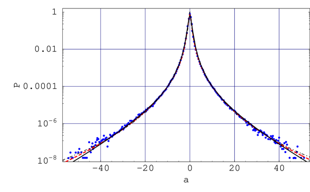
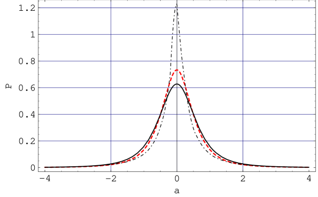
Figure 8: Lagrangian acceleration probability density function $P(a)$. Dots: experimental data for the $R_{\lambda}=690$ flow by Crawford, Mordant, Bodenschatz, and Reynolds.² Dashed line: the stretched exponential fit (4). Dot-dashed line: Beck log-normal model (25), $s=3.0$. Solid line: LDN-type model (76), $k=1$, $\alpha=1$, $D=1.130$, $B=0.163$, $\nu_{0}=2.631$, $C=1.805$. $a$ denotes acceleration normalized to unit variance.

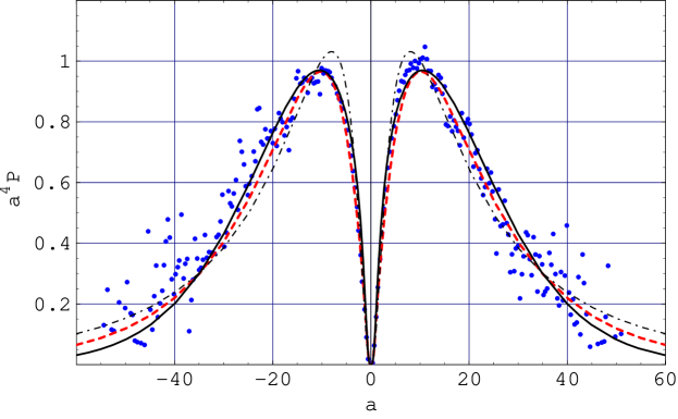
Figure 9: The contribution to fourth-order moment $a^{4}P(a)$. Same notation as in Fig. 8.

Sample fit of the dLDN probability density function $P(a)$ given by Eq. (76) and the corresponding contribution to fourth-order moment are shown in Figs. 8 and 9, respectively. In the numerical fit, we have put, in accordance to the redefinitions (63), the wave number parameter $k=1$ and the additive noise intensity parameter $\alpha=1$ in Eq. (76) and fitted the remaining three parameters $\nu_{0}$, $D$, and $B$. One can observe a good agreement with the experimental data. Particularly, the dLDN contribution to the kurtosis $a^{4}P(a)$ plotted in Fig. 9 does peak at the same points as the experimental curve (positions of the peaks depend mainly on $D$). The core of the dLDN distribution shown in Fig. 8 fits the experimental data to a higher accuracy as compared with the log-normal model (25) but yet underestimates that of the experimental curve. This departure could be attributed to the approximation of $\delta$-correlated multiplicative noise used in the dLDN model (see discussion in Sec. 4.1 above).

Having the general symmetric form of the dLDN distribution evaluated explicitly, Eq. (76), one can derive the acceleration moments $\langle a^{n}\rangle$, $n=2,4,\dots$ The associated integrals are not analytically tractable and can be evaluated numerically. We will consider these below in Sec. 5.

In the most general case ($\lambda\not=0$) the resulting $P(a)$ is given due to an exponential of the exact result (A) which will be considered below in Sec. 5.

To sum up, we have made an important step forward with the dLDN model by having calculated $P(a)$ exactly (see Appendix). We have shown that the dLDN model is capable to reproduce the recent Lagrangian experimental data on the acceleration statistics to a good accuracy. Particularly, we found that the predicted fourth-order moment density function does peak at the same value of acceleration, $|a|/\langle a^{2}\rangle^{1/2}\simeq 10.2$, as the experimental curve, in contrast to the predictions of the other considered stochastic models. The presence of the $\delta$-correlated multiplicative noise and the nonlinearity (turbulent viscosity) in the Langevin-type equation was found to be of much importance. The considered RIN models provide less but yet acceptable accuracy of the low-probability tails although they employ only one free parameter, which can be fixed by certain phenomenological arguments, as compared to the dLDN model, which contains four free parameters. However, we stress that in contrast to the LDN model the considered RIN models have a meager support from the turbulence dynamics.

5 Lagrangian acceleration statistics conditional on the velocity

In a recent paper Mordant, Crawford, and Bodenschatz[3] reported experimental data on the probability density function $P(a|u)$ of the transverse acceleration conditional on the same component of Lagrangian velocity.

Sawford, Yeung, Borgas, Vedula, Porta, Crawford, and Bodenschatz[47] have studied acceleration statistics from laboratory measurements and direct numerical simulations in 3D turbulence at $R_{\lambda}$ ranging from 38 to 1000. For large $|u|$, the conditional acceleration variance was argued to behave as

$$\langle a^{2}|u\rangle\sim u^{6},$$ (77)

obtained to a leading order in the same component $u$ (to be not confused with the rms velocity $\bar{u}\equiv\langle u^{2}\rangle^{1/2}$). This is qualitatively consistent with the stretched exponential tails of the unconditional acceleration PDF. The conditional mean rate of change of the acceleration derived from the data has been shown consistent with the drift term in second-order Lagrangian stochastic models of turbulent transport. The correlation between the square of the acceleration and the square of the velocity has been shown small but not negligible.

In a recent paper Reynolds[40] developed a self-consistent second-order stochastic model with additive noise which accounts for dependence of the Lagrangian acceleration covariance matrix $Q_{ij}=\langle a_{i}a_{j}|u\rangle$ on Lagrangian velocity $u$:

$$Q_{ij}=[f(|u|)-g(|u|)]\frac{u_{i}u_{j}}{u^{2}}+g(|u|)\delta_{ij}.$$ (78)

Here, isotropy of acceleration variances is assumed and the longitudinal and transverse functions $f(|u|)$ and $g(|u|)$ describe covariance of components in acceleration parallel and orthogonal to the velocity vector. This model extends the second-order Lagrangian stochastic model reviewed in Sec. 3.3 to account for the observed dependency of Lagrangian acceleration statistics on velocity:[3, 47]

$$da_{i}=-(T_{L}^{-1}\!+\!\tau_{\eta}^{-1})a_{i}dt+\left(\frac{1}{2}\frac{\partial Q_{ij}}{\partial u_{j}}-\sigma_{u}^{-2}Q_{ij}u_{j}\right)dt-\frac{1}{2}Q_{jk}^{-1}\frac{\partial Q_{ik}}{\partial t}a_{i}dt$$

$$+\frac{1}{2}Q_{im}\frac{\partial Q_{km}}{\partial u_{j}}a_{j}a_{k}dt+\sqrt{2\sigma_{u}^{2}(T_{L}^{-1}\!+\!\tau_{\eta}^{-1})T_{L}^{-1}\tau_{\eta}^{-1}}d\xi.$$ (79)

Fitting to the DNS data has been made by the polynomials $f=f_{0}+f_{1}u^{2}+f_{2}u^{4}+f_{3}u^{6}$ and $g=g_{0}+g_{1}u^{2}+g_{2}u^{4}+g_{3}u^{6}$.[47] The observed dependence of the conditional acceleration variance $\langle a^{2}|u\rangle$ on $u$ was partially understood in terms of Lagrangian accelerations induced by vortex tubes within which the vorticity is constant and outside which the vorticity vanishes. Dimensional arguments were invoked to derive the above third-order polynomial structure of the isotropic covariance matrix as a function of squared velocity $u^{2}$.[47] The parameters $f_{1}$, $f_{2}$, $g_{1}$, and $g_{2}$ are argued to be constants, and $f_{0}$ and $g_{0}$ are taken positive. The tails of the resulting $P(a_{i})$ can not be expressed in analytical functions but nevertheless one can show that the tails of $P(|{\bm a}|)$ have a log-normal form.

The inclusion of such conditional acceleration covariances in the model resulted in a significant reduction of the predicted occurrence of small accelerations that meets experimental and DNS data for unconditional distributions. The cores of the resulting conditional acceleration distributions were found to broaden with increasing $|u|$, in a qualitative agreement with the experiment, and in general they have almost the same shape as the unconditional distribution, in accordance with the experimental data.[3]

During the course of derivation of the generalized Fokker-Planck for single-particle Lagrangian PDF of velocity increments from the 3D Navier-Stokes equation, Friedrich[24] considered the two-point two-time acceleration autocorrelation conditional on Lagrangian velocity and position, $\langle\bm a(\bm r,t)\bm a(\bm r-\bm l,t^{\prime})|\bm u(\bm x_{0},t^{\prime}),\bm x(\bm x_{0},t^{\prime})\rangle_{\bm l=\bm v(t-t^{\prime})}$. Here, $\bm x_{0}$ is the initial position of a fluid particle. This approach and the used closure scheme were outlined in Introduction. The conditional dependence was ignored in order to get simple approximation to the diffusion term. This is consistent with K41 theory. It is of much interest to account for such a conditional dependence within the framework of this constitutive approach since experimental data and DNS show essential dependence of the Lagrangian acceleration variance on the velocity.

Recently, the multifractal approach has been used by Biferale et al.[22] to obtain acceleration moments conditional on the velocity. Particularly, the multifractal prediction

$$\langle a^{2}|u\rangle\sim u^{4.57}$$ (80)

agrees well with the DNS data for large velocity magnitudes. The exponent 4.57 differs from the value 6 predicted by Sawford et al.[47] and is very close to the Heisenberg-Yaglom scaling exponent value 9/2 entering Eq. (6). This indicates that the averaging of the conditional acceleration variance (80) over Gaussian distributed velocity $u$ is consistent with Heisenberg-Yaglom scaling law (see Eq. (68) and remark in Ref. Aringazin0305186).

The experimental data reveal highly non-Gaussian, stretched exponential character of $P(a|u)$, very similar to that of $P(a)$, for fixed $u$ ranging from zero up to about three rms velocity[3] as opposed to the theoretical result that $P(a|u)$ is a Gaussian in $a$ due to the simple RIN model (19) for arbitrary $\beta=\beta(u)$, or due to the more general RIN model (34). Similarity between the experimental $P(a|u)$ and $P(a)$ suggests that they share the process underlying the fluctuations.

Below, we consider this important problem within the framework of the general RIN approach.[46, 48]

The idea is that stretched exponential form of the tails of observed conditional distribution $P(a|u)$ could be assigned solely to small time scales, while the marginal probability distribution $P(a)$ is developed from $P(a|u)$ at large time scales, in accord to the two-time-scale dynamics.

This requires some modification in simple RIN models reviewed in Sec. 3.1. The sole use of the Gaussian-white additive noise, with fluctuating intensity depending on $u$, and a linear force $F(a)=-a$ with fluctuating $\gamma=\gamma(u)$, is not capable to explain the stretching in the observed $P(a|u)$, as it implies only Gaussian conditional probability density function $P(a|u)$, for any fixed $u$. However, it is known that accounting for the multiplicative Gaussian-white noise in the drift term of Langevin-type equation implies stretched exponential tails.

Hence one can simply follow the dLDN ansatz as a constitutive model (see Sec. 4) using the assumption that the additive noise intensity $\alpha$ appearing in the stationary probability distribution $P(a|D,\alpha,B,\nu_{0})$ given by Eq. (76) depends on $u$. Also, we will generalize consideration by taking the parameter $\lambda$ to be nonzero and depending on $u$ as well.

The stationary acceleration PDF stemming from the stochastic model (49)-(3.4) has been calculated exactly[46] and due to Eq. (A) is given by

$$P(a)=\frac{C\exp[-{\nu_{\mathrm{t}}k^{2}}/{D}+F(c,a)+F(-c,a)]}{(Da^{2}\!-\!2\lambda a\!+\!\alpha)^{1/2}(2Bka+\nu_{\mathrm{t}}k^{2})^{{2B\lambda k}/{D^{2}}}},$$ (81)

for constant parameters. Here, $C$ is normalization constant and $\nu_{\mathrm{t}}=\nu_{\mathrm{t}}(a)$, $F(c,a)$ and $c$ are given by Eqs. (A)-(108). The distribution (81) is characterized by the presence of exponential cutoff, complicated power-law dependence, and terms responsible for a skewness of the distribution (asymmetry with respect to $a\to-a$). While the skewness generation can not be directly applied to our one-dimensional case, we do not set $\lambda$ to zero for some reasons to be explained below.

One way when comparing the model predictions with experiment is to make a direct fit of the obtained PDF (81) to the experimental data on unconditional acceleration distribution by assuming all the parameters and wave number to be constant (see Sec. 4).

Particularly, this implies a reduction of the original 1D LDN model since wave number is taken to be fixed so that the artificial 1D compressibility aimed to model RDT stretching effect in 1D case is not considered. We note that the Lagrangian acceleration is usually associated with the dissipative scale, and in the present paper we do not study dependence of the parameters on the wave number. Such a dependence for velocity increments was analyzed in Ref. Laval0101036 with the expected result that for larger scales the velocity increment PDF tends to a Gaussian form. The Gaussian form is reproduced also when $D\to 0$ and $B\to 0$, i.e. the process becomes purely additive with a linear drift term.

Without loss of generality one can put, in a numerical study, $k=1$ and the additive noise intensity $\alpha=1$ by rescaling the multiplicative noise intensity $D>0$, the turbulent viscosity parameter $B>0$, the kinematic viscosity $\nu_{0}>0$, and the cross correlation parameter $\lambda$. The particular cases $B=0$ and $\nu_{0}=0$ at $\lambda=0$, and the general case at $\lambda=0$ were studied in detail in Sec. 4. Nonzero $\lambda$ is responsible for an asymmetry of the PDF (81) and in 3D picture corresponds to a correlation between stretching and vorticity (the energy cascade). Particularly, in the Eulerian framework the third-order moment of spatial velocity increment $\langle(\delta_{l}u)^{3}\rangle$ was found to be proportional to cross-correlation parameter, in accord to a kind of generalized Kármán-Howarth relationship.[44]

However, the approximation based on constant parameters does not allow one to consider both the conditional and unconditional acceleration statistics within the same model.

In the following Section, we will consider an extension of the model (49)-(56) with the solution (81) by assuming certain model parameters in the obtained stationary acceleration PDF to be dependent on random velocity.[48]

This extension is compatible with the 3D LDN approach as $\xi$ and $\sigma_{\perp}$ depend on velocity and contain large-scale quantities due to their definitions (51) and (52). Such a functional dependence and the associated longtime fluctuations have been ignored when making the simplification (3.4) with constant parameters $D$, $\alpha$, and $\lambda$. We partially restore them. This is the main point of our subsequent consideration, and the functional form of the distribution is thus due to Eq. (81) with certain parameters being now treated as functions of stochastic velocity $u$. Observations are that the acceleration variance does depend on the same component of velocity.

We point out that characteristic time of variation of the parameters should be sufficiently large to justify the approximation that the resulting PDF (81) is used with independent randomized parameters, $P(a|\textrm{Parameters})$. Two well separated timescales in the Lagrangian velocity increment autocorrelation have been established both by experiments and DNS.[4] The large timescale has been found of the order of the Lagrangian integral scale and corresponds to a magnitude part that is in accord to our assumption that the intensity of noise along the trajectory is longtime fluctuating.

5.1 LDN-type model of the conditional acceleration statistics

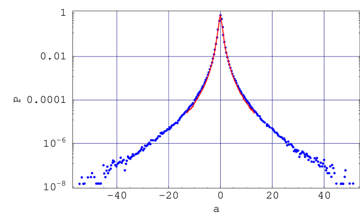
Figure 10: A comparison of the experimental unconditional Lagrangian acceleration PDF (dots) by Crawford, Mordant, Bodenschatz, and Reynolds² and the experimental conditional Lagrangian acceleration PDF at Lagrangian velocity $u=0$ (line) by Mordant, Crawford, and Bodenschatz.³ $a$ denotes acceleration normalized to unit variance.

5.1.1 Conditional and unconditional Lagrangian acceleration distributions

The experimental conditional and unconditional distributions, which we denote for brevity by $P_{\mathrm{expt}}(a|u)$ and $P_{\mathrm{expt}}(a)$ respectively, were found to be approximately of the same stretched exponential form and both reveal a strong Lagrangian turbulence intermittency. In Fig. 10 we compare $P_{\mathrm{expt}}(a|0)$ and $P_{\mathrm{expt}}(a)$.[3] This similarity indicates that they share the same process underlying the intermittency.

Accordingly, in our previous studies[46, 56, 81, 82] reviewed in Sec. 4 we used the result of a direct fit of the PDF (81) to $P_{\mathrm{expt}}(a)$, which was measured with a high precision: 3% relative uncertainty for $|a|/\langle a^{2}\rangle^{1/2}\leq 10$.[2, 3] We assumed that the parameters $\alpha$ and $\lambda$ entering Eq. (81) depend on the amplitude of Lagrangian velocity $u$, while $D$, $B$, and $\nu_{0}$ are taken to be fixed at the fitted values ($k=1$). Theoretically, only $\alpha$ and $\lambda$ may depend on velocity due to Eqs. (51) and (52), while the other parameters not.

An exponential form of $\alpha(u)$ has been proposed in Ref. Aringazin0305186 and was found to be relevant from both K62 phenomenological and experimental points of view. Particularly, such a form leads to the log-normal RIN model when $u$ is independent zero-mean Gaussian distributed,[36] and yields the acceleration PDF whose low-probability tails are in a good agreement with experiments.[34, 46] Also, we used an exponential form of $\lambda(u)$ so that the conditional acceleration PDF (81) takes the form

$$P(a|u)=P(a|\alpha(u),\lambda(u)).$$ (82)

Such a form was found to provide good fits of (i) the conditional probability density function $P(a|u)$ to $P_{\mathrm{expt}}(a|u)$; (ii) the conditional acceleration variance $\langle a^{2}|u\rangle$; and (iii) the conditional mean acceleration[81] $\langle a|u\rangle$ at various $u$ that meet the experimental data.[3] A brief report on these results is presented in Ref. Aringazin0311098.

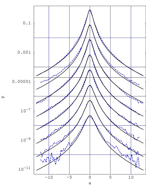
Figure 11: Theoretical conditional Lagrangian acceleration PDF $P(a|u)$ (line) and the experimental conditional Lagrangian acceleration PDF (dashed line) at velocities $u=$ 0, 0.45, 0.89, 1.3, 1.8, 2.2, 2.7, 3.1 (from top to bottom, shifted by repeated factor 0.1 for clarity) by Mordant, Crawford, and Bodenschatz.³ Lagrangian acceleration and velocity components $a$ and $u$ are normalized to unit variances.

However, self-consistent consideration of the model assumes different strategy:[48] $P(a|u)$ should be fitted to $P_{\mathrm{expt}}(a|u)$ and the marginal PDF computed due to

$$P_{\mathrm{m}}(a)=\int_{-\infty}^{\infty}P(a|u)g(u)du,$$ (83)

where $g(u)$ is PDF of independent random velocity, should reproduce $P_{\mathrm{expt}}(a)$. The marginal distribution (83) corresponds to a convolution of the stationary acceleration statistics with (independent) random velocity.

The task is thus to fit a variety of the experimental data, both on the conditional and unconditional statistics of acceleration, with a single set of fit parameters. For this purpose we use the following natural steps.

First we fit $P(a|u)=P(a|\alpha(u),\lambda(u))$ given by Eq. (81) to $P_{\mathrm{expt}}(a|u)$ assuming that the parameters depend on $u$ in an exponential way,

$$\alpha(u)=\alpha_{0}\exp[{|u|/u_{\alpha}}],\quad\lambda(u)=\lambda_{0}\exp[{|u|/u_{\lambda}}].$$ (84)

Hereafter, we use acceleration $a$ and velocity $u$ normalized to unit variances. The fit parameter set is $D>0$, $\nu_{0}>0$, $B>0$, $\lambda_{0}$, $u_{\alpha}>0$, and $u_{\lambda}>0$ ($\alpha_{0}=1$, $k=1$). The relations in Eq. (84) mean that the additive noise intensity and the correlation between the noises become higher for increasing amplitude of velocity.

We fit $P(a|0)$ to $P_{\mathrm{expt}}(a|0)$, that excludes the free parameters $u_{\alpha}$ and $u_{\lambda}$ from consideration, by varying $D$, $\nu_{0}$, and $B$ at $\alpha_{0}=1$ and $\lambda_{0}=-0.005$. We notice that the available conditional statistics $P_{\mathrm{expt}}(a|u)$ is low for high velocities, the presented acceleration range is small, $-14<a<14$, so that a rather big uncertainty remains when determining fit values of the parameters. Changes in shape of $P_{\mathrm{expt}}(a|u)$ with $u$ increasing from $u=0$ to $u=3.1$ are captured independently by the fit parameters $u_{\alpha}$ and $u_{\lambda}$. The result is shown in Fig. 11. Good overlapping of each theoretical curve with data points at all fixed magnitudes of $u$ has been achieved.

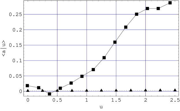
Figure 12: Theoretical conditional Lagrangian acceleration mean $\langle a|u\rangle$ (triangles) and the experimental conditional Lagrangian acceleration mean by Mordant, Crawford, and Bodenschatz³ (squares) as functions of the Lagrangian velocity $u$ normalized to unit variance.

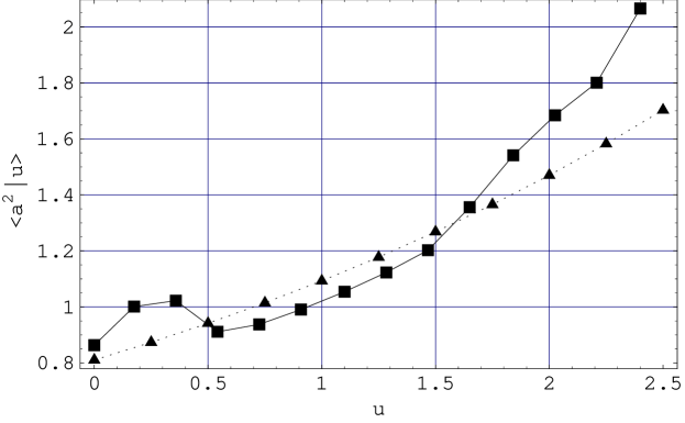
Figure 13: Theoretical conditional Lagrangian acceleration variance $\langle a^{2}|u\rangle$ (triangles) and the experimental conditional Lagrangian acceleration variance by Mordant, Crawford, and Bodenschatz³ (squares) as functions of the Lagrangian velocity normalized to unit variance.

Second we calculate the conditional mean $\langle a|u\rangle$ and the conditional variance $\langle a^{2}|u\rangle$ and compare them with the experimental data. This decreases uncertainty in fit parameter values. The results are shown in Figs. 12 and 13. Note that the predicted conditional mean $\langle a|u\rangle$ as a function of $u$ appears to be very small and does not match the experiment when the variance is fitted. We will discuss this large discrepancy in Sec. 5.1.2 below.

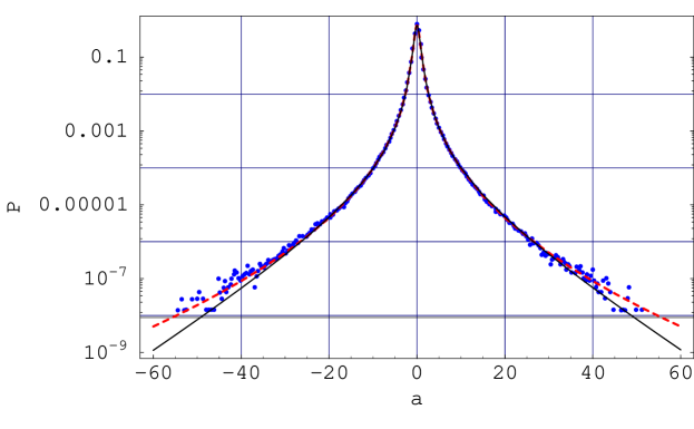
Figure 14: Theoretical marginal Lagrangian acceleration probability density function (83) with Gaussian distributed Lagrangian velocity (line), experimental data for the $R_{\lambda}=690$ flow (dots) by Crawford, Mordant, Bodenschatz, and Reynolds,² and the stretched exponential fit (4) (dashed line).

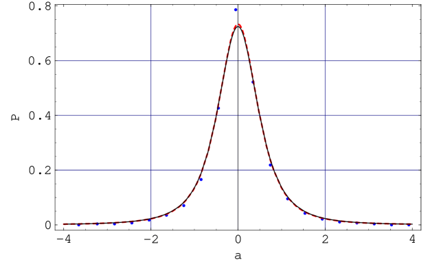
Figure 15: Lin-lin plot of the central part of the curves of Fig. 14. Same notation as in Fig. 14.

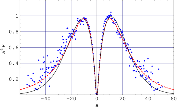
Figure 16: The contribution to fourth-order moment, $a^{4}P(a)$. Same notation as in Fig. 14.

Finally we calculate the marginal distribution $P_{\mathrm{m}}(a)$ defined by Eq. (83) by using the conditional PDF $P(a|\alpha(u),\lambda(u))$ and Gaussian distribution of velocity,

$$g(u)=\frac{1}{\sqrt{2\pi}}\exp\left[-\frac{u^{2}}{2}\right],$$ (85)

at fixed $a$. In the numerical calculation we use $a$ ranging from $-100$ to 100 with the step 0.1. Then we make an interpolation of the obtained points and fit the resulting curve to $P_{\mathrm{expt}}(a)$. A noticeable effect of the integration over $u$ with Gaussian $g(u)$ is a widening of tails of the distribution that meets the experimental data shown in Fig. 10. The used integration range for velocity is finite, $-20\leq u\leq 20$.

The fit of $P_{\mathrm{m}}(a)$ to $P_{\mathrm{expt}}(a)$ strongly decreases the uncertainty but the most strict determination of fit values comes due to a comparison of the theoretical contribution to fourth-order moment, $a^{4}P(a)$, with the experimental data. The results are shown in Figs. 14, 15, and 16. Quality of these sample fits is better than in the other recent stochastic models reviewed in Ref. Aringazin0305186. In particular, the core of the unconditional distribution reproduces very well that given by the stretched exponential (4) as one can see from Fig. 15. However, both curves a bit underestimate the height at $a=0$. This means that there is small overestimation in the range of medium accelerations, from $a=10$ to 30.

The value $\lambda_{0}=-0.005$ has been obtained by adjusting the theoretical curve to slightly different heights of the peaks of the observed $a^{4}P(a)$ shown in Fig. 16. Note that the model does not assume the use of ad hoc skewness of the forcing. Nonzero cross correlation parameter $\lambda$ naturally results not only in nonzero mean acceleration but also in a skewness of both the theoretical distributions $P(a|u)$ and $P_{\mathrm{m}}(a)$. One should extract acceleration components parallel to the velocity vector and transverse to it, to verify whether there is skewness in their distributions.

This skewness could be associated with the Eulerian downscale skewness generation, which despite of being small for homogeneous flows is known to be of a fundamental character in the inertial range (Kolmogorov four-fifth law), since the Eulerian velocity structure function $\langle(\delta_{l}u)^{3}\rangle$ was found to be related to cross-correlation between two noises. However, we stress that the observed very small skewness of acceleration distribution is attributed to the effect of anisotropy of the studied flow. How the large-scale anisotropy affects smallest scales of the flow is an interesting problem. Our fit made by using nonzero $\lambda$ is of an illustrative character, to verify whether it can explain the observed increase of the conditional mean acceleration with increasing velocity shown in Fig. 12. This issue requires a separate study and will be discussed further in Sec. 5.1.2.

Anisotropic aspects of turbulent statistical fluctuations by using irreducible representations of SO(3) group, which represents a rotational symmetry of the forceless 3D Navier-Stokes equation, have been reviewed in a recent paper by Biferale and Procaccia.[19] They stressed that the anisotropy associated with anisotropic large-scale forcing decays upon going to smaller and smaller scales of a high-Re flow, and the conflicting experimental measurements on the decay of anisotropy are explained and systematized, in an agreement with the SO(3) decomposition theory.

The following remarks are in order. Our finding is that the condition $u_{\alpha}\leq u_{\lambda}$ provides a convergence of $P_{\mathrm{m}}(a)$. Also, $u_{\lambda}$ should not be small to provide assumed condition $\lambda\ll\alpha$ at arbitrary $u$ (the cross correlation is small as compared to both noise intensities $\alpha$ and $D$).[44, 46] We used these criteria when making the fits.

The resulting sample fit values are given by

$$D=2.1,\ \nu_{0}=5.0,\ B=0.35,$$

$$\lambda_{0}=-0.005,\ u_{\alpha}=3.0,\ u_{\lambda}=3.0,$$ (86)

with $\alpha_{0}=1$ and $k=1$. The theoretical curves in Figs. 11–16 are shown for this sample set of values, which require a further fine tuning. Such a small value of $|\lambda|$ as compared to $\alpha$ or $D$ is in agreement with that obtained in the LDN direct numerical simulations. The calculated flatness factor $F=49.3$ of $P_{\mathrm{m}}(a)$ is in agreement with the experimental value (5).

To summarize, the considered Navier-Stokes equation based 1D toy model (81)-(84) is capable to fit all the available high-precision experimental data on the conditional and unconditional Lagrangian acceleration statistics[1, 2, 3] with the single set of parameters (5.1.1) to a good accuracy, with an exception being only the conditional mean acceleration, which we will consider below.

5.1.2 Conditional mean acceleration

As one can see from Fig. 12, at the values of fit parameters (5.1.1) the predicted conditional mean acceleration $\langle a|u\rangle$ qualitatively is in agreement but greatly deviates from the experimental data. Namely, it is nonzero due to nonzero $\lambda$ and increases with the increase of $|u|$ but remains to be much smaller than the experimental data even at high values of $|u|$. The conditional mean acceleration is evidently zero for a symmetrical distribution (i.e. at $\lambda=0$) and should be zero for statistically homogeneous isotropic turbulence when one studies acceleration components aligned to fixed directions. The observed departure from zero is thought to reflect large-scale anisotropy of the studied $R_{\lambda}=690$ flow. Remarkably, the DNS of (approximately) homogeneous isotropic turbulence[3] also reveals slightly nonzero mean. In Refs. Biferale0402032,Biferale0403020 a priori statistical equivalence between all the acceleration components in the laboratory frame of reference was used and the subsequent averaging over the three components gives zero-mean acceleration to a good accuracy. The latter procedure is partially justified by the high-Re effect of anisotropy decay when going to smaller scales.[19]

To reduce the discrepancy, one can try the value $u_{\lambda}=1.0$ instead of $u_{\lambda}=3.0$ to provide faster increase of $|\lambda|$ for higher $|u|$. This implies a good fit to the experimental conditional mean acceleration (see, e.g. Fig. 2 in Ref. Aringazin0311098) but we found an excess asymmetry of $P(a|u)$ at high $|u|$, with big departure from observations, and divergencies when calculating $P_{\mathrm{m}}(a)$.[48] The reason of the divergency is that $\lambda(u)$ at $u_{\lambda}=1.0$ grows faster than $\alpha(u)$ at $u_{\alpha}=3.0$ so that $\lambda$ becomes comparable or bigger than $\alpha$ with increasing $u$, and when $\lambda^{2}\to D\alpha$ the function $F(c)$ defined by Eq. (A) undergoes unbound growth. Thus we conclude that the observed nonzero conditional mean acceleration may be due to a persistent effect of the flow anisotropy rather than some intrinsic dynamical (cascade) mechanism associated with the developed turbulence. It should be emphasized however that some aspects of anisotropic fluctuations in high-Re flows were found to be universal.[19]

In general one observes a rather small relative increase of the experimental conditional mean acceleration for higher $|u|$ that eventually reflects a coupling of the acceleration to large scales of the studied flow.[23, 44] This coupling could be accounted for particularly by introducing a correlation between the Lagrangian acceleration and velocity. This possibility is of much interest to explore as it may yield the deficient increase of $\langle a|u\rangle$ but it is beyond the scope of the present formalism, which assumes an independent velocity statistics. We note also that in contrast to the experimental data on the variance $\langle a^{2}|u\rangle$ the experimental $\langle a|u\rangle$ exhibits small asymmetry with respect to $u\to-u$ (not shown in Fig. 12).[3]

The multiplicative noise intensity $D$ was taken to be independent on the velocity $u$. The effect of variation of $D$ has been considered in Ref. Aringazin0305186 with the qualitative result that it does not provide the specific change in shape of $P(a|u)$ observed in experiments as shown in Fig. 11. However, a weak dependence of $D$ on $u$ can not be ruled out.

5.1.3 Summary

In summary, the presented 1D LDN-type stochastic toy model with the velocity-dependent additive noise intensity and cross correlation parameter is shown to capture main features of the observed conditional and unconditional Lagrangian acceleration statistics to a good accuracy except for the discrepancy in the conditional mean acceleration which can be attributed to certain coupling of the acceleration to large scales of the studied $R_{\lambda}=690$ flow.[1]

One of the technical advantages of this model is that one obtains the conditional acceleration distribution in an explicit analytical form, Eq. (81), that enables to trace back all the produced effects and perform integration over velocity.

The main result is of course not only good sample fits of a variety of experimental data which are important to test performance of the model but also certain advance in understanding of the mechanism of Lagrangian intermittency provided by the dynamical Laval-Dubrulle-Nazarenko approach to small-scale turbulence.

The central point is that the LDN toy model has a deductive support from Navier-Stokes turbulence. The obtained exact analytic result for the conditional acceleration distribution and the use of recent high-precision Lagrangian experimental data on conditional and unconditional acceleration statistics allow one to make a detailed analysis of the mechanism within the adopted framework.

Effects of large scales and turbulent viscosity have been found of much importance in steady-state Lagrangian acceleration statistics. The detailed study of conditional acceleration statistics reveals a specific model structure of the external large-scale dynamics and nonlocal inter-scale coupling for homogeneous high-Re flows. Namely, the additive noise $\sigma_{\perp}$ associated with the downscale energy transfer mechanism encodes the main contribution to velocity dependence of the acceleration statistics.

In general, a cross correlation between model additive and multiplicative noises, associated with a correlation between stretching and vorticity in the 3D case, naturally provides a skewness of distributions and a nonzero mean. Weakness of this correlation measured by the parameter $\lambda$ is a theoretical requirement that meets the Lagrangian and Eulerian experiments and DNS of homogeneous isotropic turbulence. It was shown that the observed conditional mean acceleration is not related to non-zero $\lambda$ and may be attributed to flow anisotropy effects. In the Eulerian frame, the cross correlation between noises is related to the four-fifth Kolmogorov law but the effect of skewness generated by $\lambda\not=0$ is negligibly small as the result of relatively large intensity of the additive noise, which tends to symmetrize acceleration distributions. This is a dynamical evidence implied by the model rather than a result of a priori local isotropy in the spirit of K41 theory.

The use of exponential dependence of certain noise parameters on statistically independent Gaussian distributed Lagrangian velocity has been found appropriate to cover new experimental data on conditional statistics and subsequently to transfer from the conditional to unconditional acceleration distribution both exhibiting a strong Lagrangian intermittency of the flow. Such a dependence is also compatible with the log-normal statistics assumed by K62 theory and obtained in the SDT model.[76] Gaussian-white multiplicative noise and a longtime correlated intensity of Gaussian-white additive noise were both found to make essential contributions to intermittent bursts of acceleration.

It is worthwhile to mention new aspect of stochastic dynamics emerging from fluctuating character of the intensity $\alpha$ of additive noise in the presence of the multiplicative noise. The ratio between intensities of these noises, $b^{2}=D/\alpha$, controls the character of dynamics of fluid particle. For $b\ll 1$ or $b\gg 1$ the acceleration evolution is dominated by the influence of additive or multiplicative noise respectively. Since $b$ is longtime correlated stochastic parameter, the dynamics can be of a Brownian-like ($b\ll 1$), burst ($b\gg 1$), or mixed ($b\simeq 1$) character. The regimes of dynamics alternate randomly due to random $\alpha$ and are characterized by different chances of occurrence of bursts of acceleration. Relative weight of each of the regimes in a statistically stationary consideration is controlled by the ascribed distribution of $\alpha$.

The additive sector of stochastic forces entering the Langevin-type equation (49) for the acceleration is of the form $e^{u(t)}L(t)$, where $L(t)$ is Gaussian-white noise and $u(t)$ is an independent stationary process with independent increments associated with Lagrangian velocity. The stochastic process related to such representation has been recently considered by Muzy and Bacry[49] in the context of multifractal random walk[83, 84] with uncorrelated increments. We will discuss this interesting observation[36] in Sec. 6 below.

6 Multifractal random walk and Lagrangian velocity

In our previous studies[36, 46, 48] we took Lagrangian velocity component $u$ in a stationary turbulent flow to be Gaussian distributed with zero mean, i.e. $u(t)$ is understood as an independent stationary Gaussian process. For Gaussian distributed $u$ the characteristic parameter is the rms velocity ${\bar{u}}$, which completely determines statistical properties of the zero-mean random $u$. The latter is an agreement with approximately Gaussian form of the experimental curve for both of two measured components of Lagrangian velocity in developed turbulent flows.[1, 86]

In this Section, we go beyond the Gaussian modeling of the 1D process $u(t)$ by adopting the following assumption. Lagrangian velocity $u(t)$ is an independent stationary stochastically continuous process with independent increments, i.e. the increments $u(t_{1})-u(t_{0})$, $u(t_{2})-u(t_{1})$, $u(t_{3})-u(t_{2})$, $\dots$, for $t_{k+1}>t_{k}$ are uncorrelated and the joint distribution of $u(t_{0}+t)$, $u(t_{1}+t)$, $u(t_{2}+t)$, $\dots$, for any $t_{k}$ ($k=0,1,2,\dots,n$) and any $n$ does not depend on time $t$.

In essence, this assumption restates universality of the Lagrangian velocity statistics in the inertial range, in accord to K41 similarity hypotheses formulated in the Lagrangian framework, and strictly specifies statistical properties of the stochastic process $u(t)$.

In general, stationary stochastic processes with independent increments, the simplest example of which is the usual Brownian motion, is a wide class characterized by strong Markovian property (no memory effects) and the so called infinite divisibility. The most important feature of such processes for the present consideration is that one can get a general analytic form of the characteristic function of the increments which allows one to determine all statistical properties of the process for a given stochastic measure. This enables one to use a broader class of models (as compared to the Gaussian modeling) yet having well known analytical tools developed by Kolmogorov,[87] Levy,[88] and Khinchin.[89]

By definition, for stationary infinitely divisible processes the characteristic function $\varphi(z)$ of the distribution of $u(s+t)-u(s)$ can always be represented as $\varphi(z)=e^{g(z)}$, where $g(z)$ is determined by the celebrated Levy-Khinchin formula; see Eq. (93) below. For infinitely divisible processes there always exists some function $\varphi_{n}(z)$ such that the relation

$$\varphi(z)=[\varphi_{n}(z)]^{n}$$ (87)

holds for any positive integer $n$. Indeed, one can use the representation $\varphi_{n}(z)=\exp[\frac{1}{n}\ln\varphi(z)]$, where we fix arg$\,\varphi(0)=0$ to provide uniqueness of the representation.

We start by considering simple example, when the Lagrangian velocity is viewed as a stationary continuous process $u(t)$ with independent increments. In many cases, without loss of generality one can put the initial value $u(0)=0$. This process corresponds to the Brownian motion, i.e. $u(t)$ is Gaussian process with the mean $\langle u(t)\rangle=0$. We stress that this motion is not due to a molecular structure of the medium but is attributed to turbulent fluctuations. This process is stochastically continuous (of course, this does not mean that realizations of the process are continuous) and infinitely divisible. Indeed, it can be proven that in this case the increments $u(s+t)-u(s)$ are a stationary Gaussian process, i.e. $u$ is normally distributed, and the homogeneity implies independence on the value of $s$. Particularly, for the statistical law $\ln\epsilon\simeq u$ we conclude that the stochastic energy dissipation rate $\epsilon$ is log-normally distributed. This meets K62 log-normal model, in which log-normal distribution of $\epsilon$ is postulated.

Let $u(t)$ be a stationary jump process with independent increments, i.e.

$$u(t)=\mathrm{const},\textrm{ for }t\in[0,t_{1}),(t_{1},t_{2}),\dots,(t_{n},T),$$ (88)

where 0$<$$t_{1}$$<$$\cdots$$<$$t_{n}$$<$$T$ and $n$ is finite number. The velocity is constant at each of the finite-time intervals. Again, this process is stochastically continuous and infinitely divisible. It can be proven that the jump process is strongly Markovian and the number of jumps, $j(t)$, is itself a stochastically continuous stationary Poisson jump process with independent increments. With the use of $j(t)$ the process $u(t)$ can be represented as

$$u(t)=\sum_{k=1}^{j(t)}\eta_{k},$$ (89)

where $\eta_{k}$ are independent identically distributed (i.i.d) random variables, and is referred to as the generalized Poisson process.[89]

In particular, if the increments $u(s+t)-u(s)$ are a stationary Poisson process with independent increments (the characteristic function is $\varphi(z)=\exp[\lambda(e^{iz}-1)]$), we conclude that for $\ln\epsilon\simeq u$ the energy dissipation rate $\epsilon$ is log-Poisson distributed. This meets She-Leveque[90] cascade model and extended self-similarity inspired model by Dubrulle[91], which are in good agreement with the experimental data on scaling exponents of the Eulerian velocity structure functions.

In general case, a stationary stochastically continuous process with independent increments can always be decomposed into the continuous and the jump process parts.[88] Therefore, the log-Poisson distribution of $\epsilon$ stemming from the jump part of the process can receive “corrections” coming from the continuous part of the process (log-normal distribution), and vice versa. Hence, the distribution of $\epsilon$ arising from the general consideration of the stationary stochastically continuous process $u(t)$ with independent increments and the statistical law $\ln\epsilon\simeq u$ can be defined as a weighted superposition of log-Poisson and log-normal distributions. The weight parameter may depend on the scale.

Muzy and Bacry[49] has recently studied a class of log-infinitely divisible multifractal random processes of the following form:

$$X_{\tau}(t)=\int_{0}^{t}e^{\omega_{\tau}(t^{\prime})}dw(t^{\prime}),$$ (90)

where $X_{\tau}(t)=X(t+\tau)-X(t)$ is the increment of stochastic process $X(t)$, $dw(t)$ is Gaussian white-in-time noise, i.e. $w(t)$ is Wiener process, and $\omega_{\tau}(t)=\ln W_{\tau/T}(t)$. Here, $W_{\tau/T}(t)$ is a continuous version of independent identically distributed (i.i.d.) random variables of the well-known Mandelbrot’s discrete multiplicative cascade,[85] $M_{\tau}(t)=W_{\tau/\tau^{\prime}}(t)M_{\tau^{\prime}}(t)$, in the sense that the scale $\tau$ takes continuous values in replace of the discrete $\tau_{n}$. This corresponds to a continuous extension of the discrete cascade.

The stochastic process $\omega_{\tau}(t)$ can then be represented as a sum of arbitrary number of i.i.d. random variables so that by definition $\omega_{\tau}(t)$ is an infinitely divisible random process. Note that this process is defined on the scale-time $(\tau,t)$-plane, with the upper value $\tau=T$. The process $\omega_{\tau}(t)$ has the following remarkable scaling property:

$$\omega_{\lambda\tau}(\lambda t)=\omega_{\tau}(t)+\Omega_{\tau},$$ (91)

for $\lambda<1$, where $\Omega_{\tau}$ is an infinitely divisible random variable.

The multifractal random measure is defined as the small-scale limit, $M(dt)=\lim_{\tau\to 0}M_{\tau}(dt)$, of the stochastic measure $M_{\tau}(dt)=e^{\omega_{\tau}(t)}dt$. The process $M_{\tau}(t)=\int_{0}^{t}e^{\omega_{\tau}(t^{\prime})}dt^{\prime}$ is a jump process for certain choice of properties of the characteristic function of $\omega_{\tau}(t)$, namely, when the Levy measure has no Gaussian component.

The small-scale limit, $X(t)=\lim_{\tau\to 0}X_{\tau}(t)\equiv B(M(t))$, converges and is referred to as the Mandelbrot-Taylor subordinated Brownian process.[85] The process $X(t)$ represents an example of the multifractal random walk (MRW).

The MRW can thus be thought of as the usual Brownian motion defined on the “multifractal” time $\tau=M(t)$.[49] Such a viewpoint follows in general from the representation of the process $X(t)$ as the stochastic integral of a random function $f(t)=e^{\omega(t)}$ over Wiener process $w(t)$. In the case the function $f(t)$ is taken to be deterministic one ends up with the usual continuous stationary Gaussian process for $X(t)$, i.e. the Brownian motion $B(t)$ defined on usual time $t$.

The theory of one-dimensional infinitely divisible stochastic processes developed by Kolmogorov, Levy, and Khinchin was applied to the above setup. The result is that the multifractal scaling property of the absolute moments of $X(t)$ can be found exactly with the use of the Levy-Khinchin formula for the characteristic function $\varphi(z)$ of the increments of $X(t)$,

$$\varphi(z)=e^{g(z)},$$ (92)

where

$$g(z)=imz+\int(e^{izx}-1-iz\sin x)\frac{\nu(dx)}{x^{2}},$$ (93)

$\nu(dx)$ is the canonical Levy measure and $m=\langle X(t)\rangle$ is the mean. Namely, for the case of stationary multifractal measure $M(dt)$ (and finite second-order moment of the process) one has[49]

$$\langle|X(t)|^{p}\rangle=\frac{2^{p/2}\sigma^{p}\Gamma(\frac{p+1}{2})}{\Gamma(\frac{1}{2})}K_{p/2}t^{\zeta(p)},$$ (94)

where $K_{p}=T^{-\zeta(p)}\langle M^{p}\rangle$, the temporal scaling exponent is

$$\zeta(p)=\frac{p}{2}-\psi\left(\frac{p}{2}\right),$$ (95)

and the real convex cumulant-generating function $\psi(z)$ is defined by $\psi(z)=g(-iz)$, for which without loss of generality one can put $\psi(1)=0$. The intermittency parameter measures nonlinearity of $\zeta(p)$ in $p$ and is defined by

$$-\frac{\partial^{2}\zeta(p)}{\partial p^{2}}{|_{p=0}}.$$ (96)

Note also that in Eq. (94) one gets the prefactor in analytically exact form.

Mordant et al.[4] have recently demonstrated that the above MRW formalism in constructing of the additive noise in the form $e^{\omega(t)}L(t)$, which models the stochastic force having uncorrelated direction (i.e. $L(t)$ is Gaussian-white) and longtime correlation of its magnitude [i.e. $\omega(t)$ is Gaussian and ultraslow autocorrelated due to Eq. (32)], leads to the Lagrangian scaling exponent $\zeta(p)$ of the form

$$\zeta(p)=\left(\frac{1}{2}+\lambda^{2}\right)p-\frac{\lambda^{2}}{2}p^{2},$$ (97)

$\zeta(2)=1$. This corresponds to the log-normal MRW with the generating function $\psi(p)=mp+\mu^{2}p^{2}/2$, where $m$ and $\mu$ are parameters. Also, the autocorrelation functions of logarithm of the amplitude of infinitesimal Lagrangian velocity increments in time are in agreement with the experimental data on tracer particle in developed turbulent flow. The fit value of the intermittency parameter was found to be $\lambda^{2}=0.115\pm 0.01$. We note that this approach does not include a multiplicative noise sector, such as that represented by the first term in Eq. (49). While the ultraslow autocorrelated $\omega(t)$ mimics the presence of multiplicative noise, this phenomenological approach may result in essential departures from the experimental data since the multiplicative noise, which particularly arises naturally in the LDN approach reviewed in Sec. 3.4, is not present explicitly.

We note that within the same MRW framework one can consider, alternatively, log-Poisson MRW, $\psi(p)=[m-\sin(\ln\delta)]p-\gamma(1-\delta^{p})$, which yields a different prediction for the Lagrangian scaling exponent

$$\zeta(p)=m^{\prime}p+\gamma(1-\delta^{p}),$$ (98)

where $m^{\prime}$, $\gamma$, and $\delta$ are parameters. For $\delta\to 1$ and $\gamma(\ln\delta)^{2}\to\lambda^{2}$ one recovers the log-normal case. The form of this scaling exponent is similar to those of She-Leveque[90] and Dubrulle[91] cascade models corresponding to log-Poisson distribution of the normalized energy dissipation rate at spatial scale $l$,

$$\zeta^{E}(p)=(1-\Delta)\frac{p}{3}+\frac{\Delta(1-\beta^{p/3})}{1-\beta},$$ (99)

where $\Delta$ and $\beta$ are parameters, $\Delta=\beta=2/3$ corresponds to She-Leveque model and $\zeta^{E}(3)=1$; see also work by L’vov and Procaccia.[92]

The predicted Lagrangian scaling exponents can be fitted to experimental data to a good accuracy. The experimental data by Mordant et al.[29] on the relative Lagrangian scaling exponents are ($\zeta(2)=1$):

$$\zeta(p)/\zeta(2)=0.56\pm 0.01,\ 1,\ 1.34\pm 0.02,\ 1.56\pm 0.06,\ 1.8\pm 0.2$$ (100)

for $p=1,2,3,4,5$ respectively.

Recent DNS results by Biferale et al.[7] for $R_{\lambda}=280$ flow yield slightly different values: $\zeta(p)/\zeta(2)$ = 1.7$\pm$0.05, 2.0$\pm$0.05, 2.2$\pm$0.07 for $p=4,5,6$. They mention that the range of time delays over which relative scaling occurs is 10$\tau_{\eta}$ to 70$\tau_{\eta}$, and in this range anisotropic contributions induced by the large-scale flow appear to influence the scaling properties. In the range from $\tau_{\eta}$ to 10$\tau_{\eta}$ all local slopes were found to converge around the value 2. This effect is most likely due to the capture by very intense small-scale vortical structures, the relative contribution of which to the scaling properties is high in the Lagrangian frame, as compared to that in the Eulerian one. The influence of dissipative range $\tau<\tau_{\eta}$ can not be associated with these corrections since it tends to increase the value of the local slope rather than to decrease it. It was emphasized that the two-time-scale dynamics, $\tau\in[\tau_{\eta},10\tau_{\eta}]$ and $\tau\in[10\tau_{\eta},T_{L}]$, is a feature of velocity fluctuations along Lagrangian trajectories. How to incorporate such dynamical processes in the Lagrangian multifractal description and stochastic modelization of particle diffusion was mentioned as one of the most challenging open problems arising from their analysis.

In general, the above situation resembles that of fitting to the experimental Eulerian scaling exponents for which the K62 log-normal model shows an increasing departure for large orders $p$ while the She-Leveque and Dubrulle hierarchic models are in a good agreement for all experimentally accessible orders $p$. This indicates that log-Poisson models give qualitatively acceptable description of higher inhomogeneities of fully turbulent flow in the Eulerian framework.

This suggests that within the present model for the longtime behavior the jump process approximation is appropriate for qualitative and quantitative description of the random walk of the Lagrangian velocity in turbulent flow as compared with the continuous process approximation. This can be understood as the fundamental effect of finite size and finite discrete cascade mechanism of the developed turbulence.

However, both types of processes may contribute to the dynamics, and our main conclusion is that one can construct a model which includes them on equal footing by adopting the viewpoint that the process $u(t)$ is infinitely divisible with independent increments. Such a process includes both the continuous (Gaussian) and jump (Poisson) parts.

This approach could be used to address the problem pointed out recently by Chevillard et al.[23] that the Lagrangian (L) and Eulerian (E) singularity spectra $D(h)$ can not be both log-normal (parabolic), namely,

$$D^{L}(h)=-h+(1+h)D^{E}(h/(1+h)).$$ (101)

Whereas the left-hand side of the measured and DNS singularity spectrum curves for Lagrangian velocity increments are fitted, the right-hand side of them is reproduced by neither the log-normal nor the log-Poisson statistics based models mapped to the Lagrangian domain.

Here we note that this is expected result since intense and weak increments are driven by different processes related to the “burst” and “diffusive” dynamical regimes. The burst regime corresponds to capturing by very intense vortical structures while the diffusive regime describes motion in their incoherent surround. An example illustrating the difference is given by the log-normal model[34] which reproduces low-probability tails of the experimental acceleration distribution to a very good accuracy but greatly deviates (overestimates) at the central part of distribution which is characterized by low accelerations.

Within the framework of the 1D LDN model it seems to be reasonable to take the multiplicative noise $\xi$ to be Poisson distributed and use Gaussian approximation for the additive noise $\sigma_{\perp}$. We expect however robustness of the model due to the numerical results on the noisy on-off intermittency model[77] for which three quite different types of the multiplicative noise (Gauss-Markov noise produced by Ornstein-Uhlenbeck process, dichotomous noise, and chaotic noise produced by Lorenz model) were shown to produce the same power-law dependence of the moments for the model with reflective walls.

The above MRW approach gives an additional support to the representation $e^{u(t)}L(t)$ and thus to the choice $\alpha=e^{u}$, where $u$ is the magnitude of Lagrangian velocity, considered in Sec. 5. Leaving aside the choice of stochastic process for $u(t)$ (Gaussian or Poisson, or the weighted superposition of them), the difference between MRW approach by Mordant et al.[4] and RIN approach to 1D LDN-type model[46, 48] is that, in addition to the above additive noise incorporating two well separated time scales, the latter model accounts for (i) local interactions via the turbulent viscosity, (ii) the multiplicative noise effects, (iii) the coupling of additive and multiplicative noises, and (iv) the velocity-dependence of acceleration statistics.

Appendix A Exact integrals

Exact indefinite integrals, up to a constant term which does not depend on $a$, used in calculating the definite integral entering the probability density function (56) are given below.

At $\nu_{\mathrm{t}}=\nu_{0}$,

$$\int\!\!\!da\frac{-\nu_{0}k^{2}a-Da+\lambda}{Da^{2}-2\lambda a+\alpha}=-\frac{D+\nu_{0}k^{2}}{2D}\ln[Da^{2}\!-\!2\lambda a\!+\!\alpha]$$

$$+\frac{\lambda\nu_{0}k^{2}}{D\sqrt{D\alpha-\lambda^{2}}}\ \mathrm{arctan}\frac{Da-\lambda}{\sqrt{D\alpha-\lambda^{2}}}.\quad$$ (102)

At $\nu_{\mathrm{t}}=B|a|/k$, for positive (upper sign) and negative (lower sign) $a$, respectively,

$$\int da\frac{\mp Bka^{2}-Da+\lambda}{Da^{2}-2\lambda a+\alpha}=\mp\frac{Bka}{D}$$

$$-\frac{D^{2}\pm 2B\lambda k}{2D^{2}}\ln[Da^{2}-2\lambda a+\alpha]$$

$$\pm\frac{B(D\alpha-2\lambda^{2})k}{D^{2}\sqrt{D\alpha-\lambda^{2}}}\ \mathrm{arctan}\frac{Da-\lambda}{\sqrt{D\alpha-\lambda^{2}}},$$ (103)

In the general case, we have obtained a cumbersome expression

$$\int\!\!da\frac{-\nu_{\mathrm{t}}k^{2}a-Da+\lambda}{Da^{2}-2\lambda a+\alpha}=-\frac{\nu_{\mathrm{t}}k^{2}}{D}-\frac{1}{2}\ln[Da^{2}\!-\!2\lambda a\!+\!\alpha]$$

$$-\frac{2B\lambda k}{D^{2}}\ln[2Bka+\nu_{\mathrm{t}}k^{2}]+F(c)+F(-c),\quad$$ (104)

where we have denoted, for brevity,

$$F(c,a)=\frac{c_{1}k^{2}}{2c_{2}D^{2}c}\ln\left[\frac{2D^{3}}{c_{1}c_{2}(c-Da+\lambda)}\times\right.$$

$$\left.\times(B^{2}(\lambda^{2}+c\lambda-D\alpha)a+c(D\nu_{\mathrm{t}}^{2}k^{2}+c_{2}\nu_{\mathrm{t}}))\right],$$ (105)

$$c=-i\sqrt{D\alpha-\lambda^{2}},\quad\nu_{\mathrm{t}}=\sqrt{\nu_{0}^{2}+B^{2}a^{2}/k^{2}},$$ (106)

$$c_{1}=B^{2}(4\lambda^{3}+4c\lambda^{2}-3D\alpha\lambda-cD\alpha)+D^{2}(c+\lambda)\nu_{0}^{2}k^{2},$$ (107)

$$c_{2}=\sqrt{B^{2}(2\lambda^{2}+2c\lambda-D\alpha)k^{2}+D^{2}\nu_{0}^{2}k^{4}}.$$ (108)

Some useful formulas used in verifying the limits $B\to 0$ and $D\to 0$ are:

$$\mathrm{arctan}\,x=\frac{i}{2}(\ln(1-ix)-\ln(1+ix)),$$ (109)

$$\lim_{D\to 0}\frac{1}{D}\ln[1+Da^{2}]=a^{2}.$$ (110)

References

- [1] A. La Porta, G. A. Voth, A. M. Crawford, J. Alexander and E. Bodenschatz, Nature 409, 1017 (2001). G. A. Voth, A. La Porta, A. M. Crawford, E. Bodenschatz and J. Alexander, J. Fluid Mech. 469, 121 (2002); “Measurement of particle accelerations in fully developed turbulence”, physics/0110027.
- [2] A. M. Crawford, N. Mordant, E. Bodenschatz and A. M. Reynolds, “Comment on Dynamical foundations of nonextensive statistical mechanics”, physics/0212080, submitted to Phys. Rev. Lett.
- [3] N. Mordant, A. M. Crawford and E. Bodenschatz, “Experimental Lagrangian acceleration probability density function measurement”, physics/0303003.
- [4] N. Mordant, J. Delour, E. Leveque, A. Arneodo and J.-F. Pinton, Phys. Rev. Lett. 89, 254502 (2002); “Long time correlations in Lagrangian dynamics: a key to intermittency in turbulence”, physics/0206013.
- [5] T. Gotoh, D. Fukayama and T. Nakano, Phys. Fluids 14, 1065 (2002).
- [6] T. Gotoh and R. H. Kraichnan, “Turbulence and Tsallis statistics”, nlin.CD/0305040.
- [7] L. Biferale, G. Boffetta, A. Celani, A. Lanotte and F. Toschi, “Lagrangian statistics in fully developed turbulence”, nlin.CD/0402032.
- [8] N. Mordant, A. M. Crawford and E. Bodenschatz, “The 3D structure of the Lagrangian acceleration in turbulent flows”, physics/0410070.
- [9] A. N. Kolmogorov, Dokl. Akad. Nauk SSSR 30, 9 (1941).
- [10] S. Corrsin, Advances in Geophysics 6, 161 (1959).
- [11] M. Farge, G. Pellegrino and K. Schneider, Phys. Rev. Lett. 87, 054501 (2001).
- [12] A. S. Monin and A. M. Yaglom, Statistical Fluid Mechanics, Vol. 2 (MIT Press, Cambridge, MA, 1975).
- [13] W. Heisenberg, Z. Phys. 124, 628 (1948). L. D. Landau and E. M. Lifshitz, Fluid Mechanics (Addison Wisley, 1959).
- [14] H. Mouri, A. Hori and Y. Kawashima, Phys. Rev. E 70, 066305 (2004); “Vortex tubes in turbulence velocity fields at Reynolds numbers 300–1300”, physics/0407111.
- [15] U. Frisch, Turbulence: the legacy of A. N. Kolmogorov (Cambridge Univ. Press, Cambridge, 1995).
- [16] G. Falkovich, K. Gawedzki and M. Vergassola, Rev. Mod. Phys. 73, 913 (2001); “Particles and fields in fluid turbulence”, cond-mat/0105199.
- [17] E. Aurell, G. Boffetta, A. Crisanti, G. Paladin and A. Vulpiani, Phys. Rev. Lett. 77, 1262 (1996).
- [18] J. Schumacher, J. Fluid Mech. 441, 109 (2001); “Relation between shear parameter and Reynolds number in statistically stationary turbulent shear flows”, nlin.CD/0405001. J. Schumacher, K. R. Sreenivasan and P. K. Yeung, Phys. Fluids 15, 84 (2003).
- [19] L. Biferale and I. Procaccia, “Anisotropy in turbulent flows and in turbulent transport”, nlin.CD/0404014.
- [20] B. L. Sawford, Phys. Fluids A3, 1577 (1991). S. B. Pope, Phys. Fluids 14, 2360 (2002).
- [21] A. N. Kolmogorov, J. Fluid. Mech. 13, 82 (1962). L. D. Landau and E. M. Lifschitz, Fluid mechanics, 2nd Ed. (Pergamon Press, Oxford, 1987).
- [22] L. Biferale, G. Boffetta, A. Celani, B. J. Devenish, A. Lanotte and F. Toschi, “Multifractal statistics of Lagrangian velocity and acceleration in turbulence”, nlin.CD/0403020.
- [23] L. Chevillard, S. G. Roux, E. Leveque, N. Mordant, J.-F. Pinton and A. Arneodo, Phys. Rev. Lett. 91, 214502 (2003); “Lagrangian velocity statistics in turbulent flows: effects of dissipation”, cond-mat/0310105.
- [24] R. Friedrich, Phys. Rev. Lett. 90, 084501 (2003).
- [25] A. M. Oboukhov, Advances in Geophysics 6, 113 (1959).
- [26] S. B. Pope, Turbulent flows (Cambridge University Press, Cambridge, 2000).
- [27] B. Sawford, Annual Rev. Fluid Mech. 33, 289 (2001).
- [28] B. M. O. Heppe, J. Fluid Mech. 357, 167 (1998).
- [29] N. Mordant, P. Metz, O. Michel and J.-F. Pinton, Phys. Rev. Lett. 87, 214501 (2001); “Measurement of Lagrangian velocity in fully developed turbulence”, physics/0103084.
- [30] L. Chevillard, B. Castaing and E. Leveque, “On the rapid increase of intermittency in the near-dissipation range of fully developed turbulence”, cond-mat/0311409.
- [31] T. Arimitsu and N. Arimitsu, Phys. Rev. E61, 3237 (2000); J. Phys.: Condensed Matter 14, 2237 (2002); “Multifractal analysis of various PDF in turbulence based on generalized statistics: a way to tangles in superfluid He”, cond-mat/0306042.
- [32] C. Tsallis, J. Stat. Phys. 52, 479 (1988).
- [33] C. Beck, Phys. Rev. Lett. 87, 180601 (2001); “Generalized statistical mechanics and fully developed turbulence”, cond-mat/0110073.
- [34] C. Beck, “Lagrangian acceleration statistics in turbulent flow”, cond-mat/0212566.
- [35] A. K. Aringazin and M. I. Mazhitov, “Gaussian factor in the distribution arising from the nonextensive statistics approach to fully developed turbulence”, cond-mat/0301040.
- [36] A. K. Aringazin and M. I. Mazhitov, Phys. Lett. A313, 284 (2003); “The PDF of fluid particle acceleration in turbulent flow with underlying normal distribution of velocity fluctuations”, cond-mat/0301245.
- [37] B. Hnat, S. C. Chapman and G. Rowlands, “Intermittency, scaling and the Fokker-Planck approach to fluctuations of the solar wind bulk plasma parameters as seen by WIND”, physics/0211080.
- [38] A. M. Reynolds, Phys. Fluids 15, L1 (2003).
- [39] A. M. Reynolds, Phys. Rev. Lett. 91, 084503 (2003).
- [40] A. M. Reynolds, Physica A340, 298 (2004).
- [41] A. M. Reynolds, Phys. Fluids 15, 2773 (2003).
- [42] A. M. Reynolds, K. Yeo and C. Lee, Phys. Rev. E69, 067301 (2004).
- [43] A. M. Reynolds and M. Veneziani, Phys. Lett. A327, 9 (2004).
- [44] J.-P. Laval, B. Dubrulle and S. Nazarenko, Phys. Fluids 13, 1995 (2001); “Non-locality and intermittency in 3D turbulence”, physics/0101036.
- [45] J.-P. Laval, B. Dubrulle and J.C. McWilliams, Phys. Fluids 15, 1327 (2003).
- [46] A. K. Aringazin and M. I. Mazhitov, Phys. Rev. E69, 026305 (2004); “One-dimensional Langevin models of fluid particle acceleration in developed turbulence”, cond-mat/0305186.
- [47] B. L. Sawford, P. K. Yeung, M. S. Borgas, P. Vedula, A. La Porta, A. M. Crawford and E. Bodenschatz, Phys. Fluids 15, 3478 (2003).
- [48] A. K. Aringazin, Phys. Rev. E70, 036301 (2004); “Conditional Lagrangian acceleration statistics in turbulent flows with Gaussian distributed velocities”, cond-mat/0312415.
- [49] J.-F. Muzy and E. Bacry, Phys. Rev. E66, 056121 (2002); “Multifractal stationary random measures and multifractal random walks with log-infinitely divisible scaling laws”, cond-mat/0206202.
- [50] E. Bacry and J.-F. Muzy, “Log-infinitely divisible multifractal processes”, cond-mat/0207094.
- [51] A. M. Yaglom, Sov. Phys. Dokl. 11, 26 (1966).
- [52] B. B. Mandelbrot, J. Fluid. Mech. 62, 305 (1974).
- [53] E. A. Novikov, Phys. Fluids A2, 814 (1994).
- [54] D. I. Pullin and P. G. Saffman, Ann. Rev. Fluid Mech. 30, 31 (1998).
- [55] Z. Zh. Zhanabaev, S. B. Tarasov, A. K. Imanbaeva and N. E. Almasbekov, Teplofiz. i Aeromech. 9, 201 (2002).
- [56] A. K. Aringazin, “Skewness of probability density functions of fluid particle acceleration in developed turbulence”, cond-mat/0305459.
- [57] C. Beck, Physica A277, 115 (2000); Phys. Lett. A287, 240 (2001); Europhys. Lett. 57, 329 (2002); “Non-additivity of Tsallis entropies and fluctuations of temperature”, cond-mat/0105371.
- [58] R. Johal, “An interpretation of Tsallis statistics based on polydispersity”, cond-mat/9909389.
- [59] G. Wilk and Z. Wlodarczyk, Phys. Rev. Lett. 84, 2770 (2000).
- [60] A. K. Aringazin and M. I. Mazhitov, Physica A325, 409 (2003); “Quasicanonical Gibbs distribution and Tsallis nonextensive statistics”, cond-mat/0204359.
- [61] C. Beck and E. G. D. Cohen, Physica A322, 267 (2003); “Superstatistics”, cond-mat/0205097.
- [62] A. K. Aringazin and M. I. Mazhitov, “Phenomenological Gaussian screening in the nonextensive statistics approach to fully developed turbulence”, cond-mat/0212642.
- [63] B. Castaing, Y. Gagne and E. J. Hopfinger, Physica D46, 177 (1990).
- [64] Ch. Renner, J. Peinke and R. Friedrich, “On the interaction between velocity increment and energy dissipation in the turbulent cascade”, physics/0211121. Ch. Renner, J. Peinke, R. Friedrich, O. Chanal and B. Chabaud, Phys. Rev. Lett. 89, 124502 (2002).
- [65] A. A. Donkov, A. D. Donkov and E. I. Grancharova, “The exact solution of one Fokker-Planck type equation used by R. Friedrich and J. Peinke in the stochastic model of a turbulent cascade”, math-ph/9807010.
- [66] P.-O. Amblard and J.-M. Brossier, Eur. Phys. J. B12, 579 (1999).
- [67] D. H. Zanette and M. A. Montemurro, Phys. Lett. A324, 383 (2004).
- [68] S. C. Chapman, G. Rowlands and N. W. Watkins, “The origin of universal fluctuations in correlated systems: explicit calculation for an intermittent turbulent cascade”, cond-mat/0302624.
- [69] B. Portelli, P. C. W. Holdsworth and J.-F. Pinton, “Intermittency and non-Gaussian fluctuations of the global energy transfer in fully developed turbulence”, cond-mat/0112503.
- [70] S. B. Pope and Y. L. Chen, Phys. of Fluids A2, 1437 (1990).
- [71] P. K. Yeung and S. B. Pope, J. Fluid Mech. 207, 531 (1989).
- [72] M. S. Borgas, T. K. Flesch and B. L. Sawford, J. Fluid Mech. 279, 69 (1997).
- [73] B. W. Zeff, D. D. Lanterman, R. McAllister, R. Roy, E. J. Kostelich and D. P. Lathrop, Nature 421, 146 (2003).
- [74] S. Nazarenko, N. K.-R. Kevlahan and B. Dubrulle, Physica D139, 158 (2000).
- [75] B. R. Pearson, T. A. Yousef, N. E. L. Haugen, A. Brandenburg and P.-A. Krogstad, “The ‘zeroth law’ of turbulence: isotropic turbulence simulations revisited”, physics/0404114; Phys. Rev. E70, 056301 (2004).
- [76] B. Dubrulle, J.-P. Laval, S. Nazarenko and O. Zaboronski, “A model for rapid stochastic distortions of small-scale turbulence”, physics/0304035.
- [77] H. Nakao, “Asymptotic power law of moments in a random multiplicative process with weak additive noise”, cond-mat/9802030.
- [78] Y. Kuramoto and H. Nakao, Phys. Rev. Lett. 76, 4352 (1996); 78, 4039 (1997).
- [79] S. Nazarenko, R. J. West and O. Zaboronski, “Statistics of Fourier modes in the Kazantsev-Kraichnan dynamo problem”, submitted to Phys. Rev. E.
- [80] R. J. Hill, Phys. Rev. Lett. 89, 174501 (2002).
- [81] A. K. Aringazin, “The conditional mean acceleration of fluid particle in developed turbulence”, cond-mat/0306022. A. K. Aringazin and M. I. Mazhitov, “Langevin type model of the conditional Lagrangian acceleration in small-scale turbulence”, to appear in Izvestiya Vuzov (2004).
- [82] A. K. Aringazin and M. I. Mazhitov, “Stochastic model of the conditional acceleration of a fluid particle in developed turbulence”, cond-mat/0311098, accepted to Proceedings of the 21st International Congress of Theoretical and Applied Mechanics, Warsaw, 2004.
- [83] J.-F. Muzy, J. Delour and E. Bacry, Eur. J. Phys. B17, 537 (2000).
- [84] E. Bacry, J. Delour and J.-F. Muzy, Phys. Rev. E64, 026103 (2001).
- [85] B. B. Mandelbrot and H. M. Taylor, Op. Research 15, 1057 (1967).
- [86] C. Poulain, N. Mazellier, P. Gervais, Y. Gagne and C. Baudet, “Lagrangian vorticity and velocity measurements in turbulent jets”, cond-mat/0306005.
- [87] A. N. Kolmogorov, Atti Acad. Lincei 15, 805, 808, 866 (1932).
- [88] P. Levy, Ann. Scuola Norm. Pisa 2, 337 (1934).
- [89] A. Khinchin, Asymptotic laws of probability theory (ONTI, 1936).
- [90] Z. S. She and E. Leveque, Phys. Rev. Lett. 72, 336 (1994).
- [91] B. Dubrulle, Phys. Rev. Lett. 73, 959 (1994).
- [92] V. L’vov and I. Procaccia, Phys. Rev. E62, 8037 (2000).