Metal-insulator transition in a two-dimensional electron system:
the orbital effect of in-plane magnetic field

Abstract

The conductance of an open quench-disordered two-dimensional (2D) electron system subject to an in-plane magnetic field is calculated within the framework of conventional Fermi liquid theory applied to actually a three-dimensional system of spinless electrons confined to a highly anisotropic (planar) near-surface potential well. Using the calculation method suggested in this paper, the magnetic field piercing a finite range of infinitely long system of carriers is treated as introducing the additional highly non-local scatterer which separates the circuit thus modelled into three parts — the system as such and two perfect leads. The transverse quantization spectrum of the inner part of the electron waveguide thus constructed can be effectively tuned by means of the magnetic field, even though the least transverse dimension of the waveguide is small compared to the magnetic length. The initially finite (metallic) value of the conductance, which is attributed to the existence of extended modes of the transverse quantization, decreases rapidly as the magnetic field grows. This decrease is due to the mode number reduction effect produced by the magnetic field. The closing of the last current-carrying mode, which is slightly sensitive to the disorder level, is suggested as the origin of the magnetic-field-driven metal-to-insulator transition widely observed in 2D systems.

I Introduction

The conduction properties of low-dimensional electron and hole systems with the disorder of different origin have long been the subject of active research. Investigations into such objects of mesoscopic size have currently become particularly intensive in view of their applied importance (semiconductor heterostructures, quantum dot devices, etc.), on the one hand, and due to the intriguing uncommonness of the obtained results, on the other. The most puzzling phenomenon which has not as yet been understood in full measure is the transition of 2D electron systems from conducting to insulating state (the extensive bibliography on the subject can be found in Refs. bib:AbKrSar01 ; bib:KrSar04 ). Observation of this phenomenon evidently contradicts the common view stemming from the well-known scaling theory of localization bib:AALR79 .

A diversity of ideas have been put forward to explain the “anomalous” metallic behaviour of 2D systems at extremely low temperatures. Among physical mechanisms assumed to be responsible for such behaviour the most appropriate is the Coulomb ($e$-$e$) interaction of carriers. The assumption is mainly based on the fact that the dimensionless parameter $r_{s}$ (the ratio of interaction energy to Fermi energy of electrons) which characterizes this interaction amounts to the value of $\gtrsim 10$ in planar systems of Si MOSFET-type as well as in GaAs/AlGaAs heterostructures, which would suffice to raise serious doubts about the adequacy of Fermi-liquid approach with regard to such systems.

Note that in condensed matter physics an important paradigm is the quasi-particle notion. A number of phenomena can be understood in terms of weakly interacting quasi-particles, although Coulomb interaction between the electrons is rather strong. The Fermi liquid description of quasi-particles has for a long time been considered to be efficient in low dimensions in the presence of disorder bib:LR85 ; bib:CKL87 until recent experiments have challenged this view bib:KKFPdI94 . Serious problems have also arisen when interpreting numerous experimental data on decoherence time saturation at low temperature, reviewed in Ref. bib:LB02 , as well as explaning unexpectedly large persistent currents in normal metals bib:Moh99 .

At this stage, the lack of a comprehensive theory for strongly correlated electrons does not allow for certain conclusions to be made about the role of $e$-$e$ interaction in the detected phenomena. Since in different existing theories this interaction is evaluated quite differently, viz. from promoting localization bib:AAL80 ; bib:TC89 to preventing its appearance bib:F84 ; bib:BK94 ; bib:CCL98 , it would be quite reasonable at first to describe the observed effects in frames of one-particle approach and then to regard Coulomb interaction as the added dephasing factor. Only should one fail in obtaining the proper result on this canonical way may it be rational to think of Coulomb correlations as a prevalent cause of forming the continuous component in the electron spectrum of 2D systems.

Previously bib:Tar00 , the one-particle theory capable of explaining the conducting ground state of weakly disordered finite-size 2D systems was developed in terms of electron states pertinent to open quantum wells of waveguide configuration. According to this theory, the conductance must exhibit non-exponential coordinate dependence at any length of the system provided that there exists more than one extended mode of transverse quantization (so called waveguide mode), commonly referred to as the open conducting channel bib:Been97 . In Ref. bib:Tar00 it was proven that scattering by static random potential, even though it is of elastic nature from the viewpoint of one-electron dynamics, may well result in dephasing the initially coherent extended collective modes. This leads to the reduction in the primordially finite-value ballistic conductance rather than it grows from the “localized” exponentially small value. The primordial conductance is quantized in steps, each being equal to the conductance quantum $G_{0}=e^{2}/\pi\hbar$, regardless of the length of the bounded 2D system of carriers. Inclusion of imperfections allowing for scattering between different extended waveguide modes results in the conductance decrease from ballistic to diffusive value. The expression for the diffusive conductance tends asymptotically to the standard Drude form if the quantum waveguide is sufficiently wide. The above scenario of the conducting state of a real 2D electron system is evidently opposite to the one stemming from well-known scaling theory, in which the metallic behaviour of the conductance can only result from some kind of dephasing of the electron states initially localized by disorder.

Using the approach taken in Ref. bib:Tar00 , in Ref. bib:Tar03 one-particle theory of the metal-insulator transition (MIT) in 2D systems was developed. This theory provides a deeper insight into the peculiarities of the effect observed experimentally. According to bib:Tar03 , (i) MIT detected in Si-MOSFETs as well as in structures of GaAs/AlGaAs-type should be regarded as a true quantum phase transition which takes place both in disordered and perfect systems; (ii) straight from the metallic side of the transition the conductance reaches the value equal, by the order of magnitude, to the standard conductance quantum (theoretically, in the limit of an ideally perfect system, the conductance jumps exactly by $G_{0}$ as the last conducting channel is closed).

The results bib:Tar00 ; bib:Tar03 were obtained in the Fermi-liquid description of the electron system, without taking explicitly into account Coulomb interaction of carriers as well as spin effects. Meanwhile, the very fact that the extended waveguide modes were used as the initial quasi-particles (which have unlimited spatial extent, in contrast to Anderson-localized states) permits hoping that the results of Refs. bib:Tar00 ; bib:Tar03 will hold true, at least qualitatively, even on condition that Coulomb correlations are also taken into account.

Although the model of 2D MIT suggested in Ref. bib:Tar03 correlate well with the main experimental facts, it does not seem to be rather convincing to make far-reaching conclusions. The problem of great concern, which has not been touched upon in bib:Tar03 and has not been so far explained theoretically is the unusual nature of the strong localizing effect produced by the relatively weak in-plane magnetic field. Normally, the magnetic field is known to suppress the conductance of bulk metallic samples due to coupling to the orbital motion of electrons. However, if the field is applied parallel to a confined system whose actual thickness is small as compared to the magnetic length, it is natural to expect the orbital effect to be highly suppressed. Only corrections from $e$-$e$ interaction of carriers are retained in the case of spinless electrons bib:LR85 .

With this prevailing point of view, it came as a surprise when dramatic suppression of conductivity was observed in Si-MOSFETs subjected to the in-plane magnetic field bib:DKSK92 . The effect of this field was found to be so significant that it causes the zero-field 2D metal to become an insulator bib:SKSP97 ; bib:MZVSK01 ; bib:SKK01 ; bib:GMRPW02 . Inasmuch as magnetic fields appropriate for such a transition are strong enough to completely polarize electron spins, this prompted many of the researchers (see, e. g., Refs. bib:SHPLRRSG98 ; bib:OHKY99 ; bib:Metal99 ) to assert categorically that it is exactly the spin polarization that should be regarded as a physical origin of 2D MIT in a parallel magnetic field. This point of view is also supported by the lack of a comprehensive theory of the electron transport in real quasi-two-dimensional (Q2D) systems, i. e. planar systems of finite, though rather small, thickness. Although in some papers (e. g., bib:DSHw00 ; bib:MFA02 ) the orbital effect of an in-plane magnetic field was, in a way, analyzed as well, the results are still not rated as fully convincing. This is probably concerned, on the one hand, with the fact that the relatively simple model proposed in bib:DSHw00 is incapable of explaining a quite abrupt transition over the magnetic field between metallic and dielectric regimes. On the other hand, the results obtained in Ref. bib:MFA02 only exhibit the trend in behaviour of the Q2D system conductance with a growth in the magnetic field, since the applied calculation method enables one to analyze only weak-localization corrections in the metallic phase, thus being incapable of capturing the coarse effect such as MIT.

In this paper, the orbital effect of in-plane magnetic field upon open quasi-2D electron systems of waveguide configuration is investigated using the theoretic-field method previously employed in Refs. bib:Tar00 ; bib:Tar03 . The advantage of the approach is that it enables one to take into account in a similar fashion all the one-electron states, without distinguishing them by the kind of trajectories, which in Q2D case can be either of sliding type (Levi flights) or those frequently scattered at side boundaries of the system. Although the method is widely applicable, here we will examine thoroughly the specific case of weak electron-impurity scattering and weak magnetic fields (the appropriate criteria are listed below).

The notion of weak magnetic field implies the certain relationship between geometric parameters of the electron waveguide and the classical cyclotron radius of electron trajectories. At the same time, in general it does not imply low mixing of the electron states. The magnetic-field-induced mode entanglement may be rather strong, but it does not give rise to noticeable dephasing of the transverse-quantized states unless there exists some random short-correlated potential as well. The most important effect of the magnetic field is that it influences significantly the mode content of the electron spectrum, thereby resulting in noticeable change in the number of current-carrying modes and in spectral width of their energy levels. In Ref. bib:Tar04prep , it was proven that the number of conducting channels becomes smaller when the magnetic field increases, being simultaneously accompanied by the gain in coherence of the electron states. It is just the reduction in the number of extended modes that can be viewed as the physical origin of the transition of Q2D electron system from conducting to insulating state.

To justify the sensitivity of the mode state spectrum as the major cause of the observed MIT it is necessary to trace the spectrum peculiarities in terms of the observable quantity, say, the conductance. To accomplish this task, it would be inconvenient to use the Landauer approach, since it does not look into the coherence properties of the internal spectrum of the system in question, operating it as a scattering object integrally. Therefore, in this study we apply the linear response theory bib:Kubo57 which permits us to calculate the conductance on a microscopic level.

II The model

Two-dimensional electron and hole systems in use, in view of their open property in the direction of current and the resemblance of master equation to that of the classical wave theory, can be simulated as planar quantum waveguides whose transverse design is governed by the lateral confinement potentials. Although near-surface potential wells in Si MOSFETs and GaAs/AlGaAs heterostructures are close in shape to triangular or parabolic form bib:BK94 ; bib:SarKrav99 , this fact is of minor importance for its principal application which is to restrict electron transport in the direction normal to heterophase areas, thus resulting in transverse quantization of the electron spectrum. With this consideration in mind, we assume, to simplify calculations, the Q2D system of carriers to have the form of three-dimensional planar “electron waveguide” of rectangular cross-section (see Fig. 1), which occupies the coordinate region

$$x\in(-L/2,L/2)\ ,$$

$$y\in[-W/2,W/2]\ ,$$ (1)

$$z\in[-H/2,H/2]\ .$$

The length $L$, the width $W$, and the height $H$ of the waveguide will be regarded as arbitrary, within the restrictions imposed below.

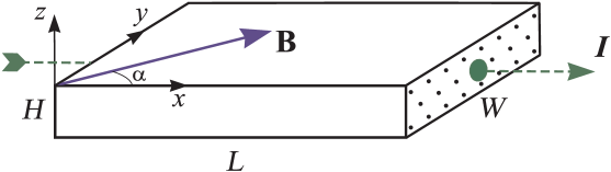
hang

Figure 1: Configuration of the electron waveguide and the magnetic field.

In practice the change of a quantum waveguide thickness implies alteration of the width of the near-surface potential well and, as a consequence, of sheet density of the carriers. Inasmuch as this density is known to follow the variation in depletion voltage under the simple law bib:S96 ; bib:WEPHAFRPJ89 , the results obtained below as a function of a waveguide thickness can be easily related to the experiment.

We will examine the $T=0$ magnetoresistance of a Q2D electron system by expressing the dimensionless (in units of $e^{2}/\pi\hbar$) conductance $g_{xx}$ in terms of one-particle propagators. Assuming the system of units with $\hbar=2m=1$ ($m$ is the electron effective mass), the static conductance is given by

$$g_{xx}(L,\mathbf{B})=\frac{2}{L^{2}}\iint\textit{d}\mathbf{r}\textit{d}\mathbf{r}^{\prime}\, \left[\frac{\partial}{\partial\,x}-\frac{ie}{\hbar c}A_{x}(\mathbf{r})\right]\left[G_{\varepsilon_{F}}^{a}(\mathbf{r},\mathbf{r}^{\prime})-G_{\varepsilon_{F}}^{r}(\mathbf{r},\mathbf{r}^{\prime})\right]$$

$$\times \left[\frac{\partial}{\partial\,x^{\prime}}-\frac{ie}{\hbar c}A_{x}(\mathbf{r}^{\prime})\right]\left[G_{\varepsilon_{F}}^{a}(\mathbf{r}^{\prime},\mathbf{r})-G_{\varepsilon_{F}}^{r}(\mathbf{r}^{\prime},\mathbf{r})\right]\ ,$$ (2)

where $G_{\varepsilon_{F}}^{r(a)}(\mathbf{r},\mathbf{r}^{\prime})$ is the retarded (advanced) Green function of the electrons of Fermi energy $\varepsilon_{F}$, $A_{i}(\mathbf{r})$ is the $i$-th component of the external vector potential $\mathbf{A}(\mathbf{r})$. Integration in (2) is performed over the region (1) occupied by the quantum waveguide, spin degeneracy is taken into account by the factor of 2. Note that throughout this paper the Fermi energy (or the chemical potential, as the situation requires) will be considered to have a constant value, independently of the confinement potential. This is undoubtedly true on the metallic side of the MIT discussed below. Moreover, on just-dielectric side of the transition this assertion is also valid since the “expanded” electron system, which includes the attached leads, in the static limit is on a homogeneous equilibrium state provided that its segment of interest is open, at least, partially.

Within the model of isotropic Fermi liquid, the retarded Green function of electrons subjected to a static magnetic field obeys the equation (all indices are omitted for brevity)

$$\left[\left(\nabla-\frac{2\pi i}{\Phi_{0}}\mathbf{A}(\mathbf{r})\right)^{2}+k_{F}^{2}+i0-V(\mathbf{r})\right]G(\mathbf{r},\mathbf{r}^{\prime})=\delta(\mathbf{r}-\mathbf{r}^{\prime})\ ,$$ (3)

where $\Phi_{0}=hc/e$ is the magnetic flux quantum, $k_{F}^{2}\equiv\varepsilon_{F}$, $V(\mathbf{r})$ is the random potential due to impurities or the roughness of the confining well boundaries. We will specify this potential by zero mean value, $\big{<}V(\mathbf{r})\big{>}=\nolinebreak 0$, and the binary correlation function $\big{<}V(\mathbf{r})V(\mathbf{r}^{\prime})\big{>}=\mathcal{QW}(\mathbf{r}-\mathbf{r}^{\prime})$. The angular brackets are used for configurational averaging, $\mathcal{W}(\mathbf{r})$ is the function normalized to unity and falling off its maximal value at $\mathbf{r}=0$ over the characteristic length $r_{c}$ (the correlation radius).

Equation (3) must be supplemented with the appropriate boundary conditions (BC). We will regard the electrons to be confined by infinitely high potential walls at side boundaries of the region (1) and specify this fact by the Dirichlet conditions as follows,

$$G(\mathbf{r},\mathbf{r}^{\prime})\bigg{|}_{\genfrac{}{}{0.0pt}{}{y=\pm W/2}{z=\pm H/2}}=0\ .$$ (4)

As far as open ends of the system are concerned, the BC problem is resolved somewhat less trivially. The mere fact that the system is open, even partially, implies non-Hermicity of the operator (3) in the domain (1). This may cause some vagueness regarding the applicability of the formula (2), whose derivation relies essentially on Hermitian property of the Hamilton operator. In the case of a finite-length system, the hermitizing BC at $x=\pm L/2$ would in fact correspond to its closeness (or periodicity) in $x$-direction, which does not conform with the requirement of current overflow between independent reservoirs.

In this study, in view of the chosen Green function formalism, to specify the openness of the quantum system we employ the method based on the analogy between the problem (3) and that of the monochromatic point source radiation in a classical waveguide. When solving the latter problem, Sommerfeld radiation conditions are normally used bib:BF78 ; bib:Vlad67 , which imply for the source positioned at some finite coordinate the existence of solely outgoing waves at infinity. In order to adapt these conditions to the system under consideration it is necessary to prolong the disordered and magnetic-field-subjected segment (1) of the electron waveguide with semi-infinite ideal leads, in which the electron waves generated at some point inside the segment could propagate freely to infinity, not being subjected to any kind of backscattering. Then, joining of the solutions to Eq. (3) at interfaces $x=\pm L/2$ within the electron waveguide results in the complete solution corresponding to the infinite open system, thereby giving rise to the correct BC at the ends of the segment of interest. This somewhat troublesome procedure will be done in the Appendix, where the trial Green functions, which serve as a basis for the exact solution to equation (3), are obtained.

Apart from the openness BC, one more problem is to be resolved before we proceed to the conductance calculation. Specifically, this is the choice of the vector potential gage corresponding to the in-plane magnetic field $\mathbf{B}=(B_{x},B_{y},0)$. Here, the main motivation is to avoid quadratic confinement in $x$-direction. The lack of such a confinement enables one to employ the transverse eigenfunction basis consisting of waveguide modes, both extended and evanescent, instead of normally used isotropic plane-wave basis. The choice of the latter basis would make the BC at side boundaries not easy to be satisfied, which would result in a substantially complicated solution. We prefer the gage

$$\mathbf{A}(\mathbf{r})=(B_{y}z,-B_{x}z,0)\ ,$$ (5)

which yields equation (3) of the form

$$\Bigg{[}\nabla^{2}+k_{F}^{2}+i0-V(\mathbf{r})-\frac{4\pi i}{\Phi_{0}}\left(B_{y}z\frac{\partial}{\partial x}-B_{x}z\frac{\partial}{\partial y}\right)-\left(\frac{2\pi}{\Phi_{0}}\right)^{2}\mathbf{B}^{2}z^{2}\Bigg{]}G(\mathbf{r},\mathbf{r}^{\prime})=\delta(\mathbf{r}-\mathbf{r}^{\prime})\ .$$ (6)

Eq. (6) is suitable for reducing the initially three-dimensional stochastic problem to a set of more readily solved one-dimensional problems. Such a reduction is particularly helpful in view of the openness BC, which is most easily formulated in one spatial dimension.

III Reduction to one-dimensional dynamic problems

Clearly, the initially three-dimensional dynamic problem might be reduced to one-dimensional problems if one succeeded, yet hypothetically, in finding the actual set of decoupled transverse eigenmodes of the random Hamiltonian in Eq. (6). As a matter of fact, one can do so, though indirectly, in terms of standard Fourier transformation of this equation over transverse vector coordinate $\mathbf{r}_{\perp}=(y,z)$. In our confinement model, the appropriate eigenfunctions are

$$\bm{|}\mathbf{r}_{\perp};\bm{\mu}\bm{\rangle}=\frac{2}{\sqrt{WH}}\sin\left[\left(\frac{y}{W}+\frac{1}{2}\right)\pi n\right]\sin\left[\left(\frac{z}{H}+\frac{1}{2}\right)\pi m\right]\ ,$$ (7)

with $\bm{\mu}=(n,m)$ being the vector mode index conjugate to $\mathbf{r}_{\perp}$ ($n,m\in\mathbb{N}$). With functions (7), equation (6) is transformed to the set of one-coordinate, yet strongly coupled, equations for the mode Fourier components of the function $G(\mathbf{r},\mathbf{r}^{\prime})$, viz.

$$\left[\frac{\partial^{2}}{\partial x^{2}}+k^{2}_{\bm{\mu}}+i0-{\mathcal{V}}_{\bm{\mu}}(x)\right]G_{\bm{\mu}\bm{\mu}^{\prime}}(x,x^{\prime})-\sum_{\bm{\nu}\neq\bm{\mu}}\hat{{\mathcal{U}}}_{\bm{\mu}\bm{\nu}}(x)G_{\bm{\nu}\bm{\mu}^{\prime}}(x,x^{\prime})=\delta_{\bm{\mu}\bm{\mu}^{\prime}}\delta(x-x^{\prime})\ .$$ (8)

Here

$$k^{2}_{\bm{\mu}}=\varepsilon_{F}-\left(\frac{\pi n}{W}\right)^{2}-\left(\frac{\pi m}{H}\right)^{2}$$ (9)

is the unperturbed mode energy,

$${\mathcal{V}}_{\bm{\mu}}(x)=V_{\bm{\mu}\bm{\mu}}(x)+\frac{H^{2}}{12l_{B}^{4}}\left(1-\frac{6}{\pi^{2}m^{2}}\right)$$ (10)

is the diagonal-in-mode-indices matrix element of the total potential which includes the disorder-induced part, $V(\mathbf{r})$, and all the magnetic-field-related terms in l.h.s. of Eq. (6), $l_{B}=\sqrt{\Phi_{0}/2\pi B}$ is the total magnetic length. The term $V_{\bm{\mu}\bm{\mu}}(x)$ in Eq. (10) is the diagonal element of the mode matrix $\|V_{\bm{\mu}\bm{\nu}}\|$, whose elements are evaluated as

$$V_{\bm{\mu}\bm{\nu}}(x)=\int_{S}\textit{d}\,\mathbf{r}_{\perp}\bm{\langle}\mathbf{r}_{\perp};\bm{\mu}\bm{|}V(\mathbf{r})\bm{|}\mathbf{r}_{\perp};\bm{\nu}\bm{\rangle}\ ,$$ (11)

integration is over cross-section $S$ of the quantum well (1). Off-diagonal matrix elements $\hat{{\mathcal{U}}}_{\bm{\mu}\bm{\nu}}(x)$ in Eq. (8) likewise include the disorder- and the magnetic-field-originated potentials,

$$\hat{{\mathcal{U}}}_{\bm{\mu}\bm{\nu}}(x)=V_{\bm{\mu}\bm{\nu}}(x)+2iH\left(\frac{S_{\bm{\mu}\bm{\nu}}^{(x)}}{l_{x}^{2}W}-\frac{S_{\bm{\mu}\bm{\nu}}^{(y)}}{l_{y}^{2}}\frac{\partial}{\partial x}\right)+C_{\bm{\mu}\bm{\nu}}\frac{H^{2}}{l_{B}^{4}}\ .$$ (12)

Here, partial magnetic lengths $l_{i}$ (with $i=y,z$) are given by $l_{i}^{2}=\Phi_{0}/2\pi|B_{i}|$, $S_{\bm{\mu}\bm{\nu}}^{(i)}$ and $C_{\bm{\mu}\bm{\nu}}$ are the model-specific numerical coefficients, each of the order unity,

$$S_{\bm{\mu}\bm{\nu}}^{(x)} = \varsigma_{x}\frac{4nn_{1}}{n^{2}-n_{1}^{2}}\sin^{2}\left[\frac{\pi}{2}(n-n_{1})\right]\big{(}1-\delta_{mm_{1}}\big{)}\frac{8mm_{1}}{\pi^{2}(m^{2}-m_{1}^{2})^{2}}\sin^{2}\left[\frac{\pi}{2}(m-m_{1})\right]\ ,$$ (13a)

$$S_{\bm{\mu}\bm{\nu}}^{(y)} = \varsigma_{y}\delta_{nn_{1}}\big{(}1-\delta_{mm_{1}}\big{)}\frac{8mm_{1}}{\pi^{2}(m^{2}-m_{1}^{2})^{2}}\sin^{2}\left[\frac{\pi}{2}(m-m_{1})\right]\ ,$$ (13b)

$$C_{\bm{\mu}\bm{\nu}} = \delta_{nn_{1}}\big{(}1-\delta_{mm_{1}}\big{)}\frac{8mm_{1}}{\pi^{2}(m^{2}-m_{1}^{2})^{2}}\cos^{2}\left[\frac{\pi}{2}(m-m_{1})\right]\ .$$ (13c)

In Eqs. (13), $\varsigma_{i}=B_{i}/|B_{i}|=\mathrm{\,sgn\,}B_{i}$ and the notations for mode indices are employed such that $\bm{\mu}=(n,m)$, $\bm{\nu}=\nolinebreak(n_{1},m_{1})$. Note that the specific form of coefficients (13) does not significantly affect the algebraic structure of Eq. (8) and hence the subsequent transformations. This fact is the main cause for the final results being uncritically sensitive to the actual form of the confinement potential.

In Eq. (8), matrix elements ${\mathcal{V}}_{\bm{\mu}}(x)$ and $\hat{{\mathcal{U}}}_{\bm{\mu}\bm{\nu}}(x)$ may be regarded as the effective potentials responsible for intra-mode and inter-mode scattering, respectively. We thus adopt the approach where interactions of the electron system with both the disorder potential and the magnetic field are exploited similarly, i. e. they are described by the additive static potentials which are basically different in their correlation properties.

To proceed further with the transverse mode decoupling, we will follow the procedure outlined in Refs. bib:Tar00 ; bib:Tar03 . It was shown there that the off-diagonal components of the mode Green matrix are expressed through corresponding diagonal elements only by means of some linear operation. Specifically, from Eq. (8) the operator relation can be derived,

$$\hat{G}_{\bm{\nu}\bm{\mu}}=\bm{P}_{\bm{\nu}}(\openone-\hat{\mathsf{R}})^{-1}\hat{\mathsf{R}}\bm{P}_{\bm{\mu}}\hat{G}_{\bm{\mu}\bm{\mu}}\ ,$$ (14)

where both $\hat{G}_{\bm{\nu}\bm{\mu}}$ and $\hat{G}_{\bm{\mu}\bm{\mu}}$ are treated as matrices in extended $x$-coordinate space $\mathbb{X}$. The operator $\hat{\mathsf{R}}$ acts in the mixed coordinate-mode space ${\mathsf{\overline{M}}_{\bm{\mu}}}$ constructed as a direct product of the space $\mathbb{X}$ and the truncated mode space which incorporates the whole set of mode indices except the unique index $\bm{\mu}$. In its turn, operator $\hat{\mathsf{R}}$ is expressed as a product of operators $\hat{G}^{(V)}$ and $\hat{\mathcal{U}}$, i. e. $\hat{\mathsf{R}}=\hat{G}^{(V)}\hat{\mathcal{U}}$, which are represented in ${\mathsf{\overline{M}}_{\bm{\mu}}}$ by matrix elements

$$\bm{\langle}x,\bm{\nu}\bm{|}\hat{\mathcal{G}}^{(V)}\bm{|}x^{\prime},\bm{\nu}^{\prime}\bm{\rangle}=G^{(V)}_{\bm{\nu}}(x,x^{\prime})\delta_{\bm{\nu}\bm{\nu}^{\prime}}\ ,$$ (15a)

$$\bm{\langle}x,\bm{\nu}\bm{|}\hat{\mathcal{U}}\bm{|}x^{\prime},\bm{\nu^{\prime}}\bm{\rangle}={\mathcal{U}}_{\bm{\nu}\bm{\nu^{\prime}}}(x)\delta(x-x^{\prime})\ .$$ (15b)

The function $G^{(V)}_{\bm{\nu}}(x,x^{\prime})$ in (15a) is the trial mode Green function which satisfies the equation resulting from (8) provided that all inter-mode potentials are put identically equal to zero,

$$\left[\frac{\partial^{2}}{\partial x^{2}}+k^{2}_{\bm{\nu}}+i0-{\mathcal{V}}_{\bm{\nu}}(x)\right]G^{(V)}_{\bm{\nu}}(x,x^{\prime})=\delta(x-x^{\prime})\ .$$ (16)

The operator $\bm{P}_{\bm{\nu}}$ in (14) is the projection operator whose action reduces to assigning the given value $\bm{\nu}$ (or $\bm{\mu}$) to the nearest mode index of arbitrary operator standing next to it (either to the left or right), without affecting the product in the $\mathbb{X}$ space. This operator may thus be thought of as contracting the action of scattering operator $\hat{\mathsf{R}}$ from three-dimensional space ${\mathsf{\overline{M}}_{\bm{\mu}}}$ to the unidirectional space $\mathbb{X}$.

Assuming $\bm{\mu}^{\prime}=\bm{\mu}$ and substituting into Eq. (8) all inter-mode propagators in the form (14) we arrive at a closed equation for the intra-mode (i. e. mode-diagonal) propagator $G_{\bm{\mu}\bm{\mu}}(x,x^{\prime})$, namely

$$\left[\frac{\partial^{2}}{\partial x^{2}}+k^{2}_{\bm{\mu}}+i0-{\mathcal{V}}_{\bm{\mu}}(x)-\hat{\mathcal{T}}_{\bm{\mu}}\right]G_{\bm{\mu}\bm{\mu}}(x,x^{\prime})=\delta(x-x^{\prime})\ ,\qquad\text{for}\ \ \forall\bm{\mu}\ .$$ (17)

Here,

$$\hat{\mathcal{T}}_{\bm{\mu}}=\bm{P}_{\bm{\mu}}\hat{\mathcal{U}}(\openone-\hat{\mathsf{R}})^{-1}\hat{\mathsf{R}}\bm{P}_{\bm{\mu}}\ ,$$ (18)

is the operator (in $\mathbb{X}$ space) potential, which in general case is highly non-local even though the magnetic-field-induced potentials may be completely non-existent. This potential bears a strong resemblance to the $T$-matrix which is well-known in quantum theory of scattering bib:Newton68 ; bib:Taylor72 . Normally, this matrix is quite singular in the multi-channel case. However, in our approach, as was proven in bib:Tar00 , the $T$-operator is properly regularized owing to separation of the intra- and inter-mode potentials in Eq. (8). We will refer below to this operator as the effective inter-mode potential.

Bearing in mind the explicit form (10) of the potential ${\mathcal{V}}_{\bm{\mu}}(x)$, in particular, the non-random nature of its “magnetic” part, it is worthwhile to renormalize unperturbed mode energy (9) by introducing, in place of $k^{2}_{\bm{\mu}}$, the magnetic-field-modified longitudinal energy

$$\varkappa_{\bm{\mu}}^{2}=k^{2}_{\bm{\mu}}-\frac{H^{2}}{12l_{B}^{4}}\left(1-\frac{6}{\pi^{2}m^{2}}\right)\ .$$ (19)

As a result, in place of equations (16) and (17) we are led to analyze a couple of different, though equivalent, equations,

$$\left[\frac{\partial^{2}}{\partial x^{2}}+\varkappa^{2}_{\bm{\nu}}+i0-V_{\bm{\nu}\bm{\nu}}(x)\right]G^{(V)}_{\bm{\nu}}(x,x^{\prime})=\delta(x-x^{\prime})\ ,$$ (20a)

$$\left[\frac{\partial^{2}}{\partial x^{2}}+\varkappa^{2}_{\bm{\mu}}+i0-V_{\bm{\mu}\bm{\mu}}(x)-\hat{\mathcal{T}}_{\bm{\mu}}\right]G_{\bm{\mu}\bm{\mu}}(x,x^{\prime})=\delta(x-x^{\prime})\ ,$$ (20b)

where solely the disorder potential $V_{\bm{\mu}\bm{\mu}}(x)$ appears instead of the total potential (10) and the replacement has been performed $k^{2}_{\bm{\mu}}\to\varkappa^{2}_{\bm{\mu}}$.

IV Spectral peculiarities of renormalized mode states

Before we proceed to the conductance calculation, let us examine fist spectral properties of the open quantum system in question, see Ref. bib:Tar04prep for more details. Although the true eigenstates are unknown in the presence of a random potential, equation (20b) permits of analyzing the particular mode state $\bm{\mu}$ comprehensively. This can be done due to one-dimensional character of the equation of motion which can be regarded as completely decoupled from the remaining bath of mode states, whatever strength of the entangling potentials in Eq. (8).

Consider the operator in square brackets of Eq. (20b), assuming equation (20a) to be ad interim solved (see Appendix) and the potential $\hat{\mathcal{T}}_{\bm{\mu}}$ thus completely determined. Our aim is to examine the average value of this operator as it specifies the energy of the particular mode in the mean-field approximation. This approximation makes practical sense on condition that scattering produced by fluctuating parts of the potentials may be regarded as weak. As far as the disorder potential $V_{\bm{\mu}\bm{\mu}}(x)$ is concerned, the weak scattering (WS) condition is normally cast to inequalities

$$k^{-1}_{F},\,r_{c}\ll\ell\ ,$$ (21)

where $\ell$ stands for the electron mean free path at a zero magnetic field. For the reference purpose, this path calculated from the model of the white-noise Gaussian-distributed potential, whose binary correlation function is $\big{<}V(\mathbf{r})V(\mathbf{r}^{\prime})\big{>}=\mathcal{Q}\delta(\mathbf{r}-\nolinebreak\mathbf{r}^{\prime})$, equals $4\pi/\mathcal{Q}$.

Given the external magnetic field, there appears an extra length parameter in the problem in question, specifically, the magnetic length, in terms of which it would be advisable to specify the condition where the magnetic-field-induced scattering could be regarded as weak. In our approach, this type of scattering is taken into consideration in two fundamentally different places. The first one is the “magnetic” part of the potential (10), which is absorbed in the mode energy renormalization (19). The other place is the mode-mixing potential (18). In this study, we will focus on the limiting case of relatively weak magnetic fields, where maximal cyclotron radius of classical electron orbit, $R_{c}~{}=~{}k_{F}l_{B}^{2}$, is large as compared to the quantum well thickness $H$. It was shown in bib:Tar04prep that under condition (21) of weak disorder-related scattering (WDS) in conjunction with the constraint

$$\left(\frac{H}{R_{c}}\right)^{2}\ll 1\ ,$$ (22)

which will be hereinafter referred to as the condition for weak magnetic scattering (WMS ), the norm of the inter-mode scattering operator $\hat{\mathsf{R}}$ in (18) is small compared to unity,

$$\|\hat{\mathsf{R}}\|^{2}\sim\frac{1}{k_{F}\ell}+\left(\frac{H}{R_{c}}\right)^{2}\ll 1\ .$$ (23)

This limitation allows the inverse operator in (18) to be expanded in series and the operator potential $\hat{\mathcal{T}}_{\bm{\mu}}$ to be simplified to the form

$$\hat{\mathcal{T}}_{\bm{\mu}}\approx\bm{P}_{\bm{\mu}}\hat{\mathcal{U}}\hat{\mathcal{G}}^{(V)}\hat{\mathcal{U}}\bm{P}_{\bm{\mu}}\ .$$ (24)

Unlike quasi-local intra-mode potential $V_{\bm{\mu}\bm{\mu}}(x)$, the potential (24) possesses a nonzero mean value, even with no magnetic field. Bearing in mind the further applications of some perturbation theory, it is advisable to divide this operator into the mean and the fluctuating parts, $\hat{\mathcal{T}}_{\bm{\mu}}=\big{<}\hat{\mathcal{T}}_{\bm{\mu}}\big{>}+\nolinebreak\Delta\hat{\mathcal{T}}_{\bm{\mu}}$. In view of definition (12), the average operator $\big{<}\hat{\mathcal{T}}_{\bm{\mu}}\big{>}$ can be split, though quite conventionally, into the sum of quasi-local “disorder” and essntially non-local “magnetic” parts, viz. $\big{<}\hat{\mathcal{T}}_{\bm{\mu}}\big{>}=\big{<}\hat{\mathcal{T}}^{(\mathcal{Q})}_{\bm{\mu}}\big{>}+\big{<}\hat{\mathcal{T}}^{(B)}_{\bm{\mu}}\big{>}$. The action of the operators $\big{<}\hat{\mathcal{T}}^{(\mathcal{Q})}_{\bm{\mu}}\big{>}$ and $\big{<}\hat{\mathcal{T}}^{(B)}_{\bm{\mu}}\big{>}$ on the Green function $G_{\bm{\mu}\bm{\mu}}(x,x^{\prime})$ is specified by equalities

$$\Big{[}\big{<}\hat{\mathcal{T}}^{(\mathcal{Q})}_{\bm{\mu}}\big{>}G_{\bm{\mu}\bm{\mu}}\Big{]}(x,x^{\prime})= \sum_{\bm{\nu}\neq\bm{\mu}}\int_{L}\textit{d}x_{1}\Big{<}V_{\bm{\mu}\bm{\nu}}(x)G^{(V)}_{\bm{\nu}}(x,x_{1})V_{\bm{\nu}\bm{\mu}}(x_{1})\Big{>}G_{\bm{\mu}\bm{\mu}}(x_{1},x^{\prime})$$ (25a)

and

$$\big{[}\big{<}\hat{\mathcal{T}}_{\bm{\mu}}^{(B)}\big{>}G_{\bm{\mu}\bm{\mu}}\big{]}(x,x^{\prime})= \sum_{\bm{\nu}\neq\bm{\mu}}\left[2iH\left(\frac{S_{\bm{\mu}\bm{\nu}}^{(x)}}{Wl_{x}^{2}}-\frac{S_{\bm{\mu}\bm{\nu}}^{(y)}}{l_{y}^{2}}\frac{\partial}{\partial x}\right)+C_{\bm{\mu}\bm{\nu}}\frac{H^{2}}{l_{B}^{4}}\right]$$

$$\times\int_{L}\textit{d}x_{1}\big{<}G^{(V)}_{\bm{\nu}}(x,x_{1})\big{>}\left[2iH\left(\frac{S_{\bm{\bm{\nu}\mu}}^{(x)}}{Wl_{x}^{2}}-\frac{S_{\bm{\nu}\bm{\mu}}^{(y)}}{l_{y}^{2}}\frac{\partial}{\partial x_{1}}\right)+C_{\bm{\nu}\bm{\mu}}\frac{H^{2}}{l_{B}^{4}}\right]G_{\bm{\mu}\bm{\mu}}(x_{1},x^{\prime})\ .$$ (25b)

To proceed further with expressions (25), it is necessary to specify the trial Green function $G^{(V)}_{\bm{\nu}}(x,x^{\prime})$ or, more precisely, its averaged value $\big{<}G^{(V)}_{\bm{\nu}}(x,x^{\prime})\big{>}$. In doing so, we will use a somewhat simplified version of correlation relations for the disorder potential, namely

$$\big{<}V(\mathbf{r})\big{>} =0\ ,$$ (26a)

$$\big{<}V(\mathbf{r})V(\mathbf{r}^{\prime})\big{>} =\mathcal{QW}(x-x^{\prime})\delta(\mathbf{r}_{\perp}-\mathbf{r}^{\prime}_{\perp})\ .$$ (26b)

As shown in the Appendix, under WS conditions which imply that WDS inequalities (21) and WMS inequality (22) are satisfied simultaneously, the averaging of the trial Green function results in the asymptotic expression

$$\big{<}G^{(V)}_{\bm{\nu}}(x,x^{\prime})\big{>}\approx\frac{-i}{2\varkappa_{\bm{\nu}}}\exp\left\{\left[i\varkappa_{\bm{\nu}}-\frac{1}{2}\left(\frac{1}{L_{f}^{(V)}(\bm{\nu})}+\frac{1}{L_{b}^{(V)}(\bm{\nu})}\right)\right]|x-x^{\prime}|\right\}\ .$$ (27)

Here, $L_{f,b}^{(V)}(\bm{\nu})$ are the forward ($f$) and the backward ($b$) scattering lengths of the trial mode $\bm{\nu}$, which are determined from model (26) as bib:Tar03

$$L_{f}^{(V)}(\bm{\nu})=\frac{4S}{9\mathcal{Q}}\left(2\varkappa_{\bm{\nu}}\right)^{2}\ ,\hskip 56.9055ptL_{b}^{(V)}(\bm{\nu})=\frac{4S}{9\mathcal{Q}}\frac{\left(2\varkappa_{\bm{\nu}}\right)^{2}}{\widetilde{\mathcal{W}}(2\varkappa_{\bm{\nu}})}\ ,$$ (28)

$\widetilde{\mathcal{W}}(q)$ is the Fourier transform of the function $\mathcal{W}(x)$ from (26b). Expression (27) is literally applicable to extended modes, i. e. to modes with $\varkappa_{\bm{\nu}}^{2}>0$. with $\varkappa_{\bm{\nu}}^{2}<0$ (evanescent modes) one should assume $\varkappa_{\bm{\nu}}=i|\varkappa_{\bm{\nu}}|$ in Eq. (27) and both of the extinction lengths (28) to turn to infinity.

With function (27), the action of the operator $\big{<}\hat{\mathcal{T}}^{(\mathcal{Q})}_{\bm{\mu}}\big{>}$ reduces to multiplying the operand in Eq. (25a) by the complex-valued disorder-related self-energy factor bib:Tar00 ; bib:Tar03 , specifically, $\Big{[}\big{<}\hat{\mathcal{T}}^{(\mathcal{Q})}_{\bm{\mu}}\big{>}G_{\bm{\mu}\bm{\mu}}\Big{]}(x,x^{\prime})=-\varSigma^{(\mathcal{Q})}_{\bm{\mu}}G_{\bm{\mu}\bm{\mu}}(x,x^{\prime})$, where $\varSigma^{(\mathcal{Q})}_{\bm{\mu}}=\Delta\varkappa_{\bm{\mu}}^{2}+i/\tau_{\bm{\mu}}^{(\varphi)}$, with

$$\Delta\varkappa_{\bm{\mu}}^{2} =\frac{\mathcal{Q}}{S}\sum_{\bm{\nu}\neq\bm{\mu}}\mathcal{P}\int_{-\infty}^{\infty}\frac{\mathrm{d}q}{2\pi}\;\frac{\widetilde{\mathcal{W}}(q+\varkappa_{\bm{\mu}})}{q^{2}-\varkappa_{\bm{\nu}}^{2}}\ ,$$ (29a)

$$\frac{1}{\tau_{\bm{\mu}}^{(\varphi)}} =\frac{\mathcal{Q}}{4S}\overline{\sum_{\bm{\nu}\neq\bm{\mu}}}\frac{1}{\varkappa_{\bm{\nu}}}\left[\widetilde{\mathcal{W}}(\varkappa_{\bm{\mu}}-\varkappa_{\bm{\nu}})+\widetilde{\mathcal{W}}(\varkappa_{\bm{\mu}}+\varkappa_{\bm{\nu}})\right]\ .$$ (29b)

Symbol $\mathcal{P}$ in Eq. (29a) stands for the integral principal value, the bar over the summation index in (29b) signifies the summation over extended modes only, if any.

The conditional character of the term “disorder self-energy” with reference to $\varSigma^{(\mathcal{Q})}_{\bm{\mu}}$ suggests that this factor is actually determined not solely in terms of the disorder potential, which results in the pre-factor of $\mathcal{Q}$, but also is influenced by the magnetic field. The latter field renormalizes wavenumbers $\varkappa_{\bm{\mu},\bm{\nu}}$ and adjusts the number of extended modes, see below. Here it should be noted that the dephasing factor (29b) can only be nonzero if quench-disorder-induced scattering is allowed between different extended modes. Otherwise the coherence of the trial mode states is unaffected by static disorder.

Apart from the disorder-induced fraction of the mode self-energy, the action of essentially non-local “magnetic” part of the operator $\big{<}\hat{\mathcal{T}}_{\bm{\mu}}\big{>}$ results in additional self-energy term which will later on be referred to as magnetic self-energy,

$$\varSigma^{(B)}_{\bm{\mu}}=\sum_{\bm{\nu}\neq\bm{\mu}} \left[2iH\left(\frac{S_{\bm{\mu}\bm{\nu}}^{(x)}}{Wl_{x}^{2}}-i\varkappa_{\bm{\mu}}\frac{S_{\bm{\mu}\bm{\nu}}^{(y)}}{l_{y}^{2}}\right)+C_{\bm{\mu}\bm{\nu}}\frac{H^{2}}{l_{B}^{4}}\right]$$

$$\times\frac{1}{\varkappa_{\bm{\mu}}^{2}-\varkappa_{\bm{\nu}}^{2}-i\varkappa_{\bm{\nu}}\left(\frac{1}{L_{f}^{(V)}(\bm{\nu})}+\frac{1}{L_{b}^{(V)}(\bm{\nu})}\right)}\left[2iH\left(\frac{S_{\bm{\nu}\bm{\mu}}^{(x)}}{Wl_{x}^{2}}-i\varkappa_{\bm{\mu}}\frac{S_{\bm{\nu}\bm{\mu}}^{(y)}}{l_{y}^{2}}\right)+C_{\bm{\nu}\bm{\mu}}\frac{H^{2}}{l_{B}^{4}}\right]\ .$$ (30)

The principal difference between the disorder and the magnetic self-energies is that the former takes a non-zero value provided that the disorder strength (which is specified by the parameter $\mathcal{Q}$) be finite. On the contrary, the magnetic-field-induced term $\varSigma^{(B)}_{\bm{\mu}}$ only vanishes in the limit of the magnetic field equal to zero, remaining otherwise finite at any disorder strength. By comparing imaginary parts of the terms $\varSigma^{(\mathcal{Q})}_{\bm{\mu}}$ and $\varSigma^{(B)}_{\bm{\mu}}$ one can determine that the ratio of “magnetic” and “disorder” dephasing rates is evaluated as

$$\frac{\Im\varSigma^{(B)}_{\bm{\mu}}}{\Im\varSigma^{(\mathcal{Q})}_{\bm{\mu}}}\sim\left[\frac{H}{R_{c}k_{F}W}\left(\frac{B_{x}}{B}\right)^{2}+\frac{H}{R_{c}}\left(\frac{B_{y}}{B}\right)^{2}+\frac{H^{2}}{R_{c}^{2}}\right]^{2}\ll 1\ .$$ (31)

It is clear that under WMS condition (22) the magnetic-field-originated dephasing is negligible, whatever level of the disorder. One is thus led to conclude that strong inter-mode mixing resulting from the magnetic field only does not cause the mode energy levels to be considerably widened unless there exists a random potential due to some kind of disorder serving as a mediator for the magnetic-field-related dephasing effect. As far as mode entanglement is concerned, it is evident from (29) that the specific role of the magnetic field is to change the collective parameters of the electron spectrum, such as the mode content of the confined system of carriers and the mode density of states (MDOS). It is only in this indirect manner that the mode level width becomes dependent on the magnetic field.

The number of extended modes in the quantum waveguide, which substantially governs dephasing rate (29b), is specified by the requirement for mode energies to be positive-valued. Prior to analyzing in WS approximation the role of fluctuating potentials $V_{\bm{\mu}\bm{\mu}}(x)$ and $\Delta\hat{\mathcal{T}}_{\bm{\mu}}$ one can notice that the energy of a specific mode depends not only on the confining potential but also on the magnetic field that likewise produces the confinement effect. As seen from (19), the new “unperturbed” mode energy $\varkappa_{\bm{\mu}}^{2}$ decreases steadily with the magnetic field growth, whatever the orientation within the plane of a 2D system. A decrease in that energy should result in truncation of the number of extended modes responsible for current transport and, therefore, in the conductance abruptly falling off. The latter effect is quite often interpreted in terms of electron effective mass enhancement bib:ADPGTV04 .

Although magnetic renormalization (19) is of purely intra-mode nature, corrections of the same sign to the mode energy are produced by the inter-mode magnetic scattering as well, which is taken into account by self-energy (30). This is indeed the case as long as WMS condition holds true. Moreover, inter-mode magnetic scattering can lead to some anisotropy of the electron effective mass with respect to the magnetic field in-plane orientation, depending on symmetry properties of numerical coefficients in Eq. (30), i. e. on geometrical symmetry of the quantum well. Note that the intra-mode magnetic term in (19) is entirely isotropic.

As the magnetic field increases, the terms in square brackets of (30), which are proportional to $C_{\bm{\mu}\bm{\nu}}$, will exceed the rest of the terms, thus resulting in the subsequent increase of the mode energy. This effect, however, corresponds to the range of relatively strong magnetic fields, where WMS inequality (22) is violated. In this paper, this case will not be dealt with.

In Figure 2, the numerical dependence of the extended mode number $N_{c}$, commonly referred to as the number of effective conducting channels,

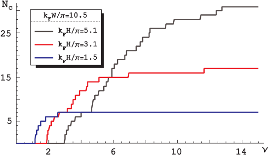
1inhang

Figure 2: The dependence of the number of extended modes in the quantum waveguide on the inverse magnetic field ($\nu$ is the Landau filling factor).

is reproduced from Ref. bib:Tar04prep . The magnetic field assumed to be codirectional with the axis of current flow is scaled as the Landau-level filling factor $\nu=\nolinebreak(k_{F}l_{B})^{2}=\nolinebreak k_{F}R_{c}$. The collapse of the number of current-carrying modes with a growing magnetic field is apparent, regardless of the quantum well thickness $H$, the width $W$ being held constant. Numerical considerations reveal that in-plane rotation of the magnetic field slightly changes the picture presented. This is consistent with the fact that the real part of self-energy (30) can reach, at most, the same value (on the order of magnitude) as the magnetic term in (19), and is in agreement with experiments bib:PBPB02 .

We also reproduce from bib:Tar04prep the $N_{c}$ dependence on the effective thickness of the quantum waveguide, the latter adjusted in practice by depletion voltage. In the lowest magnetic fields (upper curve in Fig. 3) the number of channels shows a near-linear increase with growing $H$. This corresponds to standard geometrical considerations applicable to systems of waveguide configuration. As the magnetic field is getting higher,

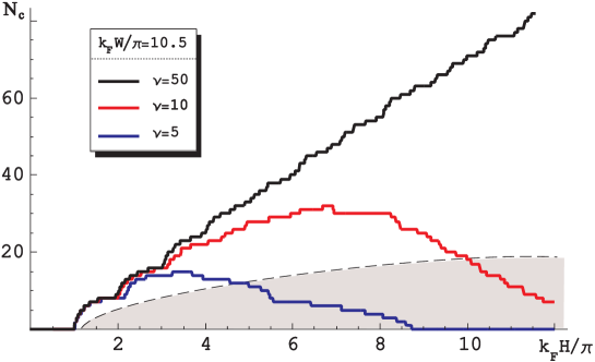
1inhang

Figure 3: The number of conducting channels vs the width of the near-surface potential well at different values of the Landau filling factor. The shaded area below the dashed curve covers the parameter region where the WMS criterion is violated.

the conventional geometric increase in the number of channels slows down, gradually changing to a decrease in the conducting mode number. This unusual non-monotonicity of the mode content of the quantum system is due to essentially non-monotonic dependence on $H$ of the magnetic-field-renormalized mode energy (19).

The parallel magnetic field effect on the number of subbands in a quantum well was previously noticed by some authors bib:SdS89 ; bib:SdS93 with reference to semiconductor heterostructures. The reduction in the number of conducting channels with a growth in the magnetic field is certainly a quantum-mechanical effect pertinent to multi-electron systems. As a matter of fact, its nature is closely related to the Aharonov-Bohm (AB) phase incursion, which is known to effectively change carriers’ energy bib:Olariu85 ; bib:Wash91 and has an impact on the interference patterns observed in experiments with AB rings. In the problem under study, unlike quasi-1D metal rings subjected to magnetic field, the AB phase is essentially different for electrons following different orbits. Therefore, it may seem to be difficult to take the magnetic field into account by conventional wave function phase renormalization. Yet this phase effect appears in the collective mode energies, affecting crucially the number of current-carrying modes in a laterally confined electron system.

The apparent impact of the in-plane magnetic field on the number of extended modes inevitably occurs in the magnetic-field dependence of the mode dephasing rate. While in the limit of a large number of conducting channels the replacement of the sum in Eq. (29b) with the integral leads to the familiar quasi-classical formula,

$$\frac{1}{\tau_{\bm{\mu}}^{(\varphi)}(B)}\approx\frac{1}{\tau_{\bm{\mu}}^{(\varphi)}(0)}\sqrt{1-\frac{H^{2}}{12R_{c}^{2}}}\ ,$$ (32)

where $1/\tau_{\bm{\mu}}^{(\varphi)}(0)=k_{F}\mathcal{Q}/4\pi$ stands for the dephasing rate due to disorder scattering in the absence of magnetic field bib:Tar03 , in Fig. 4 we give the numerically obtained dependence on the magnetic field of two particular modes of the quantum waveguide under study. Well-known van Hove singularities of MDOS, which are directly related to step-wise change in the number of extended modes, are well pronounced on both of the curves.

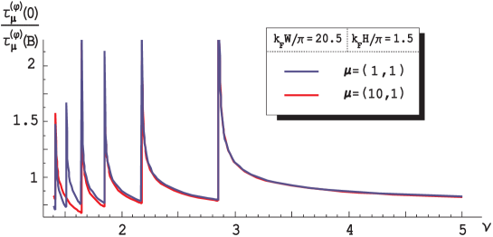
1in hang

Figure 4: The dephasing rate (29b) for two particular modes vs inverse magnetic field.

Besides, Fig. 5 illustrates the dephasing rate of the particular mode vs variable effective thickness of Q2D system of carriers. Availability of van Hove singularities similar to those depicted in Fig. 4 compels one to conclude that by means of the orbital coupling to Q2D electrons the in-plane magnetic field has the effect which is, in a way, similar to that of the electrostatic confinement potential. At the same time, in contrast to the magnetic-field-controlled singularities shown in Fig. 4, the oscillations of truly geometrical origin are noticeably more complicated. The distinction is attributed to a substantially different response of the effective mode energy (19) to the magnetic field, on the one hand, and to size parameters of the confined electron system, on the other. However, it should be emphasized that in both of the graphs, 4 and 5, the reduction of the dephasing by the

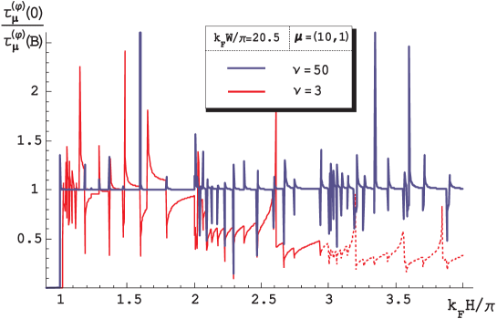
1in hang

Figure 5: The dephasing rate vs the quantum waveguide thickness at different strengths of in-plane magnetic field. The broken fraction of the lower curve falls into the range of parameters where WMS condition (22) is violated.

quenched disorder is clearly visible as the magnetic field grows. This fact is indicative of an increase in coherence of the electron transport in quench-disordered Q2D systems subjected to an external magnetic field.

V Magnetoconductance of a Q2D system

By substituting the Green functions into Eq. (2) in the form of expansion in series over transverse Hamiltonian eigenfunctions we obtain the following mode representation of the conductance,

$$g_{xx}(L,\mathbf{B})=\frac{2}{L^{2}}\iint_{L}\textit{d}x\textit{d}x^{\prime}\sum_{\ \genfrac{}{}{0.0pt}{}{\bm{\nu}_{1},\bm{\nu}_{2}}{\bm{\nu}_{3},\bm{\nu}_{4}}} \left(\frac{\partial}{\partial x}\delta_{\bm{\nu}_{1}\bm{\nu}_{2}}-i\varsigma_{y}\frac{\hat{z}_{\bm{\nu}_{1}\bm{\nu}_{2}}}{l_{y}^{2}}\right)\Big{[}G^{a}_{\bm{\nu}_{2}\bm{\nu}_{3}}(x,x^{\prime})-G^{r}_{\bm{\nu}_{2}\bm{\nu}_{3}}(x,x^{\prime})\Big{]}$$

$$\times \left(\frac{\partial}{\partial x^{\prime}}\delta_{\bm{\nu}_{3}\bm{\nu}_{4}}-i\varsigma_{y}\frac{\hat{z}_{\bm{\nu}_{3}\bm{\nu}_{4}}}{l_{y}^{2}}\right)\Big{[}G^{a}_{\bm{\nu}_{4}\bm{\nu}_{1}}(x^{\prime},x)-G^{r}_{\bm{\nu}_{4}\bm{\nu}_{1}}(x^{\prime},x)\Big{]}\ .$$ (33)

Here, $\delta_{\bm{\nu}_{i}\bm{\nu}_{j}}$ is the vector-argument Kronecker delta, $\hat{z}_{\bm{\nu}_{i}\bm{\nu}_{j}}$ is the inter-mode matrix element of the $z$-coordinate operator which, given the model of the confining potential, assumes the value

$$\hat{z}_{\bm{\nu}\bm{\nu}^{\prime}}=-H\delta_{nn^{\prime}}(1-\delta_{mm^{\prime}})\frac{8mm^{\prime}}{\pi^{2}\left(m^{2}-m^{\prime 2}\right)^{2}}\sin^{2}\left[\frac{\pi}{2}(m-m^{\prime})\right]\ ,\qquad\qquad\bm{\nu}=(n,m)\ .$$ (34)

Using interrelation (14) between off-diagonal and diagonal mode propagators, and estimate (23) for the inter-mode scattering operator it is easy to make sure that the principal contribution to (33) arises from the terms whose mode indices are coincident with one another. As a result, the conductance is expressed, asymptotically in WS limit, as

$$g_{xx}(L,\mathbf{B})\approx\frac{2}{L^{2}}\sum_{\bm{\nu}}\iint_{L}\textit{d}x\textit{d}x^{\prime}\frac{\partial}{\partial x}\Big{[}G^{a}_{\bm{\nu}\bm{\nu}}(x,x^{\prime})-G^{r}_{\bm{\nu}\bm{\nu}}(x,x^{\prime})\Big{]}\frac{\partial}{\partial x^{\prime}}\Big{[}G^{a}_{\bm{\nu}\bm{\nu}}(x^{\prime},x)-G^{r}_{\bm{\nu}\bm{\nu}}(x^{\prime},x)\Big{]}\ .$$ (35)

This formula, in conjunction with (20), ultimately reduces the initially stated three-dimensional dynamic problem to a set of decoupled, strictly 1D problems which in the general case are non-Hermitian.

Under WS conditions, equation (20b) can be solved analytically with an arbitrary accuracy in fluctuating potentials. However, there is no need to overestimate the expected result. In Refs. bib:Tar00 ; bib:Tar03 , it was proven that for inactive media with channel number $N_{c}>1$ the presence of dephasing term (29b) in the operator potential (24) enables one to neglect fluctuating potentials in Eq. (20b), thereby seeking intra-mode propagators from the deterministic equation

$$\left(\frac{\partial^{2}}{\partial x^{2}}+\varkappa^{2}_{\bm{\mu}}+i/\tau_{\bm{\mu}}^{(\varphi)}\right)G_{\bm{\mu}\bm{\mu}}(x,x^{\prime})=\delta(x-x^{\prime})\ .$$ (36)

The solution to this equation, which obeys the openness conditions at the ends of the interval $\mathcal{L}=(-L/2,L/2)$, under WS conditions is written as

$$G_{\bm{\mu}\bm{\mu}}(x,x^{\prime})\approx\frac{1}{2i\varkappa_{\bm{\mu}}}\exp\left[\left(i\varkappa_{\bm{\mu}}-1/l_{\bm{\mu}}^{(\varphi)}\right)|x-x^{\prime}|\right]\ ,$$ (37)

where $l_{\bm{\mu}}^{(\varphi)}=2\varkappa_{\bm{\mu}}\tau_{\bm{\mu}}^{(\varphi)}$ is the length of the mode $\bm{\mu}$ phase coherence. With function (37) substituted into Eq. (35), the average magnetoconductance is given as

$$\big{<}g_{xx}(L,\mathbf{B})\big{>}=\overline{\sum_{\bm{\nu}\neq\bm{\mu}}}\frac{l_{\bm{\mu}}^{(\varphi)}}{L}\left[1-\frac{l_{\bm{\mu}}^{(\varphi)}}{L}\exp\left(-\frac{L}{l_{\bm{\mu}}^{(\varphi)}}\right)\sinh\frac{L}{l_{\bm{\mu}}^{(\varphi)}}\right]\ .$$ (38)

Here, the terms corresponding to extended modes only are kept since the evanescent-mode Green functions, which are strongly localized in $x$-direction, are real-valued and cancel each other in Eq. (35). Note that formula (38) can be viewed as describing the system conductance in the presence of both the random scatterers and the magnetic field, which enters implicitly through mode coherence lengths.

From general result (38), conventional limiting formulae for the conductance can readily be obtained. In particular, in ballistic limit $L\ll\ell$ the dimensionless conductance becomes nearly equal to the number of open conducting channels,

$$\big{<}g_{xx}(L,\mathbf{B})\big{>}\approx N_{c}(\mathbf{B})\ .$$ (39)

This number, as it follows from the above analysis, is determined by both the geometric confinement of the electron system and the magnetic field, see Figs. 2 and 3. The perfect system conductance is thus expected to run in steps as a function of either depletion voltage or the value of the in-plane magnetic field.

In diffusion limit $L\gg\ell$, if the potential well in the $z$-direction is wide enough to contain the large number of quantization levels in this direction, by replacing the sum in r.h.s. of (38) with the integral we arrive at

$$\big{<}g_{xx}(L,\mathbf{B})\big{>}\approx\frac{4}{3}\frac{N_{c}(\mathbf{B})\ell}{L}\approx\big{<}g_{xx}(L,0)\big{>}\left(1-\frac{H^{2}}{12R_{c}^{2}}\right)\ .$$ (40)

In the case of the zero magnetic field this result is coincident in form with classical Drude conductance bib:Tar03 . If $\mathbf{B}\neq 0$, the magnetoconductance is negative, being varied smoothly with the magnetic field, specifically, under the quadratic law. This is because the van Hove singularities of MDOS prove to be integrated out in such a rough calculation.

However, these singularities are actually contained in the mode coherence lengths, as they are determined using the dephasing rate formula (29b). They should appear both in Shubnikov-de Haas (i. e. magnetic-field-driven) oscillations of the conductance and in the conductance dependence on the quantum well width, which is normally tuned by depletion voltage. In Fig. 6, the results numerically obtained from Eq. (38) at

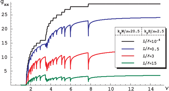
1in hang

Figure 6: The conductance vs inverse magnetic field at different disorder level in the quantum waveguide.

several values of the diffusion parameter, $L/\ell$, are presented. MDOS singularities reveal themselves in the form of sharp dips placed close to those points where the number of conducting modes undergoes stepwise variations, i. e. to the thresholds of the transverse subbands, no matter what the disorder level may be. The disorder seems to manifest itself through the absolute value of the conductance. Note that in the case of relatively large disorder (large values of $L/\ell$) the conductance develops non-monotonically vs the magnetic field, even if MDOS singularities are smoothed out. When decreasing the mean free path, non-monotonicity becomes so apparent that it appears to be inadmissible to disregard this effect in the experimental data. In particular, with regard to this analysis it would be tempting to revise the observed positive magnetoresistance which is frequently attributed to spin properties of 2D systems bib:ZMMCG02 ; bib:MinGerRSGZW03 .

To make a comparison with the magnetic-field run, in Fig. 7 the conductance is shown versus the width of the potential well forming a quasi-2D quantum waveguide. Here, MDOS singularities are equally more pronounced, which demonstrates the change in the number of conducting channels. Meanwhile, in the latter case these singularities are completely anticipated from the very outset, since the number of channels is normally associated with size quantization. The peculiar feature should be noted in Fig. 7 as against the dependence on the magnetic field. The curves in Fig. 7 tend to become non-monotonic, on average, as the magnetic field grows. Evidently, this non-monotonicity accounts for the non-monotonic dependence on $H$ of the mode eigen-energy (19).

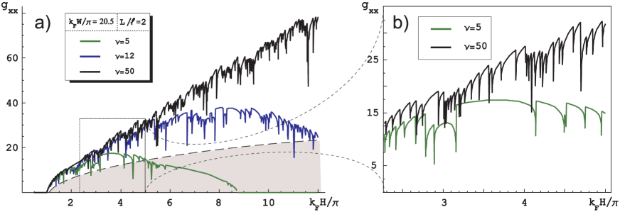
hang

Figure 7: The conductance vs the width of the near-surface potential well at different values of the in-plane magnetic field. In panel (b), the region selected by the rectangle in panel (a), with only two curves left, is zoomed in to make the dips arisen due to MDOS singularities more clearly visible. Similarly to Fig. 3, the shading below the dashed curve signifies the region where criterion (22) is violated.

It is instructive to dwell upon the physical nature of dips in Figs. 6 and 7. All of them are positioned in the vicinity of the points corresponding to opening/closing of the conducting channels. For one thing, as the electron waveguide gets thin or the magnetic field grows, the closing of the channel must result in a bench-like fall of the conductance since each of the conducting channels is expected to bring in exactly one conductance quantum. At the critical point, the edge extended mode is transformed to the evanescent one, which is localized at a scale of the mode wavelength and in this way carry no current in an infinitely long system. Indeed, this picture is demonstrated by the upper, “ballistic”, curve in Fig. 6.

For another, in approaching the transformation point (subband threshold) the MDOS of the edge mode diverges whereas its mode velocity tends to zero. The capacious and slow edge mode serves as a destructive sink for dynamic electrons, leading to a decrease in the conductance. It is clear that the dips can arise only when we deal with an imperfect system of carriers, where scattering is allowed from all remaining extended modes to the slow critical mode. The conductance in the bottom of the dip may thus reach, hyperbolically, a nearly zero value, which can hardly be grasped in real experiments because of various unaccounted extra factors.

VI Discussion and concluding remarks

We have demonstrated that the appreciable localizing effect produced by relatively weak in-plane magnetic field on 2D electron and hole systems can be reasonably interpreted in the context of Fermi liquid theory applied to spinless electrons which reside in an open near-surface potential well of finite rather than zero width. For a relatively weak magnetic field, its coupling to the carrier orbital degree of freedom, even though it is rather weak from semi-classical point of view, proves to have substantial influence on the carrier spectrum and, hence, on the conductance.

The conclusion about strong sensitivity of the carrier spectrum to the in-plane magnetic field is made from the analogy of tightly gated solid-state systems to classical wave-guiding systems of planar, though three-dimensional, configuration. The mode content of these well-known objects is quite sensitive to the anisotropy in their cross-section, that is to the applied gate voltage as far as electron devices are concerned. A remarkable feature of the latter type of systems is that in case the magnetic field is applied to the finite length, these systems can be thought of as being subjected to both the disorder potential, whose correlation length can be arbitrary, and the additive deterministic strongly non-local “magnetic” potential barrier. Scattering parameters of this barrier are specified by the magnetic field strength and orientation, on the one hand, and by the length of magnetically biased section of the quantum waveguide, on the other. The effect produced by this barrier results from the mismatching of electron spectra in the inner and outer parts of the quantum well, the inner part representing the finite-length electron system under consideration.

If the electron waveguide cross-section is strongly anisotropic, the bulk of transverse modes in the electron spectrum proves to be efficiently transformed from extended to evanescent type as the magnetic field grows slightly. This is because electron scattering from side boundaries of the confining potential well is, in the strict sense, specular if the boundaries are considered as completely inhibiting the transverse current flow. In view of this fact, it seems to be erroneous to assess the magnetic field effect on the electron system by simply estimating the variation of the electron trajectory portions between successive collisions with quantum well boundaries. It can be easily verified from Eqs.(9) and (19) that the mode truncation effect of the magnetic field is the more significant the larger is the aspect ratio of the waveguide cross-section, given the dimension $H$. For $H$ being small enough, such that only modes with quantization parameter $m=1$ in the corresponding direction can be regarded as extended, the total number of extended modes in the quantum waveguide is mainly determined by the larger cross-section dimension, $W$ in the case under study. Owing to this, even slight alteration of the magnetic field can transform a considerable number of modes from extended to evanescent type, thus leading to significant reduction of the conductance, even though it might have a large (ballistic) value in the absence of the magnetic field.

The mode truncation effect of in-plane magnetic field appears to be quite similar to that of truly geometric confinement of the electron system. The closing of each of the current-carrying modes, which makes itself evident in the form of conductance jumps by exactly one conductance quantum in a perfect system at a zero temperature, should be regarded as a true quantum phase transition bib:SGCS97 . This statement is substantiated by the indisputable fact that there exists a well-defined correlation length in the vicinity of a closing point, whose role is played by the wave length of the marginal extended mode, which tends to diverge as the critical point is approached. The closing of the last conducting mode by means of the in-plane magnetic field may thus be regarded as the magnetic-field-driven MIT.

It should be noted that in the proximity to the MIT the conductance is not quite precisely described by the present theory, since it is hard to satisfy WMS conditions over the corresponding range of system parameters. At the same time, closer examination of magnetic-field-originated items in Eq. (20b) reveals that the above-described mode truncation effect and, hence, the very fact of the existence of magnetic-field-driven MIT, is robust.

In this paper we have not focused our attention upon the conductance anisotropy with respect to in-plane orientation of the magnetic field. The corresponding analysis is straightforward. It consists in comparing the real part of anisotropic self-energy (30) and the magnetic part of the trial mode energy (19). Under WMS condition (22), both of these energy items are of the same order of magnitude, save the case of the magnetic field oriented nearly parallel to the direction of current. We thus expect the conductance anisotropy to be expressed, at most, moderately. Moreover, in view of numerical coefficients in Eq. (30) being model-specific, the conductance anisotropy in practice should be governed substantially by the confinement potential profile. It should be noted that assuming the magnetic field to grow beyond WMS limit, the isotropic terms proportional to $l_{B}^{-4}$ can be made dominating in self-energy (30), thereby removing the in-plane anisotropy of the conductance. This range of the magnetic field strength needs to be given a special consideration because the “magnetic scattering”, which is an important aspect of our approach, cannot be regarded as weak in this particular case.

Yet another relevant remark should be made concerning the model of the confinement potential adopted in this study. In some papers where laterally confined electron systems are dealt with (see, e. g., Ref.bib:DSHw00 ), this potential is taken as a quadratic function. Thus modelled confinement seems to be beneficial from the technical point of view, as it enables one to account for the magnetic field non-perturbatively, the corresponding transverse eigen-states being known as Fock-Darwin levels bib:SdS89 ; bib:SdS93 . It is natural that the precisely zero width of those levels in the absence of any disorder implies the entire lack of dephasing due to the magnetic field only. In this case, the magnetoconductance should not exhibit a dip structure because the latter results from MDOS singularities arising exclusively in the presence of the disorder.

In the domain of weak magnetic fields (in a sense of inequality (22)) the quadratic confinement can hardly be substantiated. Therefore, the issue of the magnetic-field-induced mode entanglement and the related dephasing of the mode states might seem to be quite topical in this limiting case. Note, however, that although rectangular confinement possesses appreciable inter-mode magnetic scattering, it proves not to result in widening the transverse quantization levels unless some kind of disorder is also taken into account. The exact form of transverse eigen-functions is of no fundamental significance for the development of transport theories in mode representation, but the mere fact of transverse energy quantization does matter. This prompts us to expect that the magnetic field alone cannot give rise to noticeable decoherence of electron states for any hard-wall model of the electron confinement. The specific form of the confinement potential can only alter the arrangement of transverse quantization levels and, consequently, influence the coherence properties of the electron system indirectly. Of primary value is the dephasing resulting from scattering caused by some kind of random (i. e., in a sense, uncontrolled) potential, no matter static or variable it may be.

*

Appendix A Trial mode Green function in the presence of magnetic field

A.1 Reduction of the boundary-value problem to auxiliary Cauchi problems

Prior to obtaining the proper boundary conditions for Eq. (20a), which would conform to the physical definition of the system openness at the end points $x=\pm L/2$, note that the problem governed by this equation is absolutely identical to that of point-source-radiated classical waves in an 1D random medium. Bearing this in mind, we will extend the driving equation from the finite interval $\mathcal{L}$ to the whole $x$-axis, writing it down in symbolic form

$$\left[\frac{d^{2}}{dx^{2}}+k^{2}+i0-V(x)\right]G^{(V)}(x,x^{\prime})=\delta(x-x^{\prime})\ ,$$ (41)

where the potential $V(x)$ is assumed to be the finite-support function which consists of two fundamentally different items. The regular component of this potential is $V^{(reg)}(x)=\frac{H^{2}}{12l_{B}^{4}}\left(1-\frac{6}{\pi^{2}m^{2}}\right)\theta(L/2-|x|)$, with $\theta(x)$ being the Heaviside unit-step function, whereas the additional random disorder term is $V^{(dis)}(x)=V_{\bm{\mu}\bm{\mu}}(x)\theta(L/2-|x|)$. For the sake of clarity we will omit mode index $\bm{\mu}$, implying that both the wave number $k$ in (41) and $\varkappa$ below are related exactly to this mode.

Since there is a need to perform configurational averaging over the potential $V^{(dis)}(x)$ it is worthwhile to express the solution to Eq. (41) in terms of wave functions of causal type rather than functions that comply with the initially stated boundary-value (BV) problem. This is achieved by employing the formula

$$G^{(V)}(x,x^{\prime})=\frac{1}{\mathcal{W}}\big{[}\psi_{+}(x)\psi_{-}(x^{\prime})\theta(x-x^{\prime})+\psi_{+}(x^{\prime})\psi_{-}(x)\theta(x^{\prime}-x)\big{]}\ ,$$ (42)

where $\psi_{\pm}(x)$ are two different solutions of homogeneous equation (41) with the boundary conditions specified for each of them at only one end of the coordinate axis, viz. $x\to\pm\infty$, depending on the sign index, $\mathcal{W}$ is the Wronskian of the above solutions. With this representation, the trial propagator itself satisfies, as it must, the initial BV problem and the averaging procedure can be accomplished mathematically correctly, with due account of multiple backscattering.

Inasmuch as the support of the potential in Eq. (41) is bounded, functions $\psi_{\pm}(x)$ may be sought in the form

$$\psi_{\pm}(x) =\pi_{\pm}(x)\mathrm{e}^{i\varkappa(\pm x-L/2)}-i\gamma_{\pm}(x)\mathrm{e}^{-i\varkappa(\pm x-L/2)} \text{at}\qquad|x|\leqslant L/2\ ,$$ (43a)

$$\psi_{\pm}(x) =c_{\pm}\mathrm{e}^{ik(\pm x-L/2)} \text{at}\qquad|x|>L/2\ ,$$ (43b)

where $\varkappa^{2}=k^{2}-V^{(reg)}$. Under WDS condition (21), envelope functions $\pi_{\pm}(x)$ and $\gamma_{\pm}(x)$ in (43a) can be regarded as smooth factors as compared with near-standing fast exponentials, which leads to the following coupled dynamic equations,

$$\pm\pi^{\prime}_{\pm}(x)+i\eta(x)\pi_{\pm}(x)+\zeta^{*}_{\pm}(x)\gamma_{\pm}(x)=0\ ,$$ (44a)

$$\pm\gamma^{\prime}_{\pm}(x)-i\eta(x)\gamma_{\pm}(x)+\zeta_{\pm}(x)\pi_{\pm}(x)=0\ .$$ (44b)

Random functions $\eta(x)$ and $\zeta_{\pm}(x)$ in (44) are constructed as narrow packets of spatial harmonics of the disorder potential,

$$\eta(x)=\frac{1}{2\varkappa}\int_{x-l}^{x+l}\frac{\mathrm{d}t}{2l}V^{(dis)}(t)\ ,$$ (45a)

$$\zeta_{\pm}(x)=\frac{1}{2\varkappa}\int_{x-l}^{x+l}\frac{\mathrm{d}t}{2l}V^{(dis)}(t)\exp[2i\varkappa(\pm x-L/2)]\ ,$$ (45b)

where spatial averaging is over the interval $2l$ of an arbitrary length intermediate between “small” length scales $\varkappa^{-1}$ and $r_{c}$, on the one hand, and the large scattering length (to be determined self-consistently), on the other. These limitations ensure smoothed random “potentials” $\eta(x)$ and $\zeta_{\pm}(x)$ to provide the harmonics $\pm\varkappa$ forward and backward scattering, respectively.

By joining the solutions (43a) and (43b) at the end points of interval $\mathcal{L}$ we arrive at the necessary BC for envelopes $\pi_{\pm}(x)$ and $\gamma_{\pm}(x)$, viz.

$$\pi_{\pm}(\pm L/2)= \mathrm{const}\ ,$$ (46a)

$$\gamma_{\pm}(\pm L/2)= \mathcal{R}^{(B)}\pi_{\pm}(\pm L/2)\ .$$ (46b)

The quantity

$$\mathcal{R}^{(B)}=-i\frac{k-\varkappa}{k+\varkappa}\ ,$$ (47)

as it follows from (43a), is the amplitude reflection coefficient from the interface between the magnetically biased and unbiased regions of the extended 1D quantum waveguide. This reflection will be hereinafter referred to as “magnetic scattering” associated with the above introduced potential $V^{(reg)}(x)$. It can be easily verified that under constraint (22) the reflection parameter (47) is modulo small as compared to unity.

By substituting functions $\psi_{\pm}(x)$ in the form (43a) into (42), the trial Green function whose both coordinate arguments are located inside magnetically biased interval $\mathcal{L}$ is given as

$$G^{(V)}(x,x^{\prime})=\mathcal{G}_{1}(x,x^{\prime})\mathrm{e}^{i\varkappa(x-x^{\prime})}+\mathcal{G}_{2}(x,x^{\prime})\mathrm{e}^{-i\varkappa(x-x^{\prime})}+\mathcal{G}_{3}(x,x^{\prime})\mathrm{e}^{i\varkappa(x+x^{\prime})}+\mathcal{G}_{4}(x,x^{\prime})\mathrm{e}^{-i\varkappa(x+x^{\prime})}\ ,$$ (48)

where the last two terms in r.h.s. have emerged as a direct consequence of the mode backscattering. In (48), smooth envelope functions are

$$\mathcal{G}_{1}(x,x^{\prime})=\frac{-i}{2\varkappa}\mathcal{A}(x)\left[\Theta_{+}\frac{\pi_{-}(x^{\prime})}{\pi_{-}(x)}-\Theta_{-}\frac{\gamma_{+}(x^{\prime})}{\pi_{+}(x)}\Gamma_{-}(x)\mathrm{e}^{2i\varkappa L}\right]\ ,$$ (49a)

$$\mathcal{G}_{2}(x,x^{\prime})=\frac{-i}{2\varkappa}\mathcal{A}(x)\left[\Theta_{-}\frac{\pi_{+}(x^{\prime})}{\pi_{+}(x)}-\Theta_{+}\Gamma_{+}(x)\frac{\gamma_{-}(x^{\prime})}{\pi_{-}(x)}\mathrm{e}^{2i\varkappa L}\right]\ ,$$ (49b)

$$\mathcal{G}_{3}(x,x^{\prime})=\frac{-1}{2\varkappa}\mathcal{A}(x)\mathrm{e}^{i\varkappa L}\left[\Theta_{+}\frac{\gamma_{-}(x^{\prime})}{\pi_{-}(x)}+\Theta_{-}\frac{\pi_{+}(x^{\prime})}{\pi_{+}(x)}\Gamma_{-}(x)\right]\ ,$$ (49c)

$$\mathcal{G}_{4}(x,x^{\prime})=\frac{-1}{2\varkappa}\mathcal{A}(x)\mathrm{e}^{i\varkappa L}\left[\Theta_{-}\frac{\gamma_{+}(x^{\prime})}{\pi_{+}(x)}+\Theta_{+}\Gamma_{+}(x)\frac{\pi_{-}(x^{\prime})}{\pi_{-}(x)}\right]\ ,$$ (49d)

where the notations are used

$$\mathcal{A}(x)=\left[1+\Gamma_{+}(x)\Gamma_{-}(x)\mathrm{e}^{2i\varkappa L}\right]^{-1}\ ,$$ (50a)

$$\Gamma_{\pm}(x)=\gamma_{\pm}(x)/\pi_{\pm}(x)\ ,$$ (50b)

$$\Theta_{\pm}=\theta[\pm(x-x^{\prime})]\ .$$ (50c)

The functions $\Gamma_{\pm}(x)$ play a particular role in the averaging technique. It can be deduced from Eq. (43a) that these functions are nothing but the reflection coefficients of spatial harmonics $\pm\varkappa$ which are incident at the point $x$ onto the disordered layers whose end coordinates are $x$ and $\pm L/2$, respectively. These reflection factors are well-known to obey the Riccati-type dynamic equations bib:Klyats86 ,

$$\pm\frac{\mathrm{d}\Gamma_{\pm}(x)}{\mathrm{d}x}=2i\eta(x)\Gamma_{\pm}(x)-\zeta_{\pm}(x)+\zeta_{\pm}^{*}(x)\Gamma_{\pm}^{2}(x)\ ,$$ (51)

which in our case must be supplied with “initial” conditions (one-side BC) stemming from (46), viz.

$$\Gamma_{\pm}(\pm L/2)=\mathcal{R}^{(B)}\ .$$ (52)

A.2 Configuration averaging of the function (48)

The averaging technique as applied to functionals of smoothed potentials (45) was elaborated in Refs. bib:Tar00 ; bib:MakTar01 ; bib:FreiTar01 . It relies basically on the fact that under WS conditions the functional arguments (45) can be regarded as Gaussian-distributed random variables bib:LGP82 . Taking account of correlation equalities (26), the binary correlators of these effective potentials, which would suffice to be allowed for, can be cast to the form

$$\big{<}\eta(x)\eta(x^{\prime})\big{>}=\frac{1}{L_{f}}F_{l}(x-x^{\prime})\ ,$$ (53a)

$$\big{<}\zeta_{\pm}(x)\zeta_{\pm}^{*}(x^{\prime})\big{>}=\frac{1}{L_{b}}F_{l}(x-x^{\prime})\ ,$$ (53b)

where $L_{f}$ and $L_{b}$ are the forward and backward scattering lengths given in (28) for the particular mode $\bm{\nu}$. The function

$$F_{l}(x)=\int_{-\infty}^{\infty}\frac{\mathrm{d}q}{2\pi}\mathrm{e}^{iqx}\frac{\sin^{2}(ql)}{(ql)^{2}}=\frac{1}{2l}\left(1-\frac{|x|}{2l}\right)\theta(2l-|x|)$$ (54)

is sharp on a scale of significant change in smooth amplitudes of electron wave functions, and therefore it can act as the under-limiting $\delta$-function when averaging amplitude factors $\mathcal{G}_{i}(x,x^{\prime})$ in (48). Prior to averaging these factors, it is advantageous to absorb, wherever possible, the forward-scattering field $\eta(x)$ by going over from functions $\gamma_{\pm}(x)$, $\pi_{\pm}(x)$ and $\zeta_{\pm}(x)$ to phase-renormalized functions

$$\widetilde{\gamma}_{\pm}(x) =\gamma_{\pm}(x)\exp\left[\pm i\int_{x}^{\pm L/2}\mathrm{d}x_{1}\eta(x_{1})\right]\ ,$$ (55a)

$$\widetilde{\pi}_{\pm}(x) =\pi_{\pm}(x)\exp\left[\mp i\int_{x}^{\pm L/2}\mathrm{d}x_{1}\eta(x_{1})\right]\ ,$$ (55b)

$$\widetilde{\zeta}_{\pm}(x) =\zeta_{\pm}(x)\exp\left[\pm 2i\int_{x}^{\pm L/2}\mathrm{d}x_{1}\eta(x_{1})\right]\ .$$ (55c)

An important thing is that correlation relation (53b) remains unchanged after renormalization (55c).

In view of short-range correlation of random functions (45) and due to the causal nature of functionals being averaged, the averaging of functionals with different sign indices in (49) can be done separately. By applying the Furutsu-Novikov formula for Gaussian random processes bib:Klyats86 , we first average the equation for renormalized reflection factors $\widetilde{\Gamma}_{\pm}(x)=\widetilde{\gamma}_{\pm}(x)/\widetilde{\pi}_{\pm}(x)$, i. e.

$$\pm\frac{\mathrm{d}\widetilde{\Gamma}_{\pm}(x)}{\mathrm{d}x}=-\widetilde{\zeta}_{\pm}(x)+\widetilde{\zeta}_{\pm}^{*}(x)\widetilde{\Gamma}_{\pm}^{2}(x)\ .$$ (56)

With condition (52) taken into account this yields

$$\langle\widetilde{\Gamma}_{\pm}(x)\rangle=\mathcal{R}^{(B)}\exp\left[-\frac{1}{L_{b}}\left(\frac{L}{2}\mp x\right)\right]\ .$$ (57)

In view of WMS-motivated smallness of the reflection parameter $\mathcal{R}^{(B)}$, this implies that only the terms that do not contain the factors of $\widetilde{\Gamma}_{\pm}(x)$ and $\widetilde{\gamma}_{\pm}(x)$ can be kept in (49) when averaging Green function (48).

Next, in order to average the ratio $\widetilde{\pi}_{\pm}(x^{\prime})/\widetilde{\pi}_{\pm}(x)$ consider its Fourier transform over $x^{\prime}$ coordinate,

$$\Phi^{(\pm)}(x,q)=\pm\int_{x}^{\pm L/2}\mathrm{d}x_{1}\frac{\widetilde{\pi}_{\pm}(x_{1})}{\widetilde{\pi}_{\pm}(x)}\exp\left[-iq(x-x_{1})+i\varkappa|x-x_{1}|\pm i\int_{x_{1}}^{x}\mathrm{d}x_{2}\eta(x_{2})\right]\ ,$$ (58)

where we have separated the forward-scattering random field $\eta(x)$ in the form of a phase factor. Averaging over this field yields readily

$$\Big{<}\exp\left[\pm i\int_{x_{1}}^{x}\mathrm{d}x_{2}\eta(x_{2})\right]\Big{>}_{\eta}=\exp\left(-\frac{|x-x_{1}|}{2L_{f}}\right)\ .$$ (59)

Then, after averaging over $\eta(x)$, the function (58) comes to obey the equation

$$\mp\frac{\mathrm{d}\big{<}\widetilde{\Phi}^{(\pm)}(x,q)\big{>}_{\eta}}{\mathrm{d}x}=1-\left(\frac{1}{2L_{f}}-i\varkappa\mp iq\right)\big{<}\widetilde{\Phi}^{(\pm)}(x,q)\big{>}_{\eta}-\widetilde{\zeta}_{\pm}^{*}(x)\widetilde{\Gamma}_{\pm}(x)\big{<}\widetilde{\Phi}^{(\pm)}(x,q)\big{>}_{\eta}\ ,$$ (60)

which is to be solved jointly with Eq. (56). Averaging of Eq. (60) over the effective back-scattering field $\widetilde{\zeta}_{\pm}(x)$ results in the dynamic equation

$$\mp\frac{\mathrm{d}\big{<}\widetilde{\Phi}^{(\pm)}(x,q)\big{>}}{\mathrm{d}x}=1-\left[\frac{1}{2}\left(\frac{1}{L_{f}}+\frac{1}{L_{b}}\right)-i\varkappa\mp iq\right]\big{<}\widetilde{\Phi}^{(\pm)}(x,q)\big{>}\ ,$$ (61)

which is to be solved with obvious “initial” condition, $\big{<}\widetilde{\Phi}^{(\pm)}(\pm L/2,q)\big{>}=0$. The solution to Eq. (61) yields

$$\big{<}\widetilde{\Phi}^{(\pm)}(x,q)\big{>}=\left[\frac{1}{2}\left(\frac{1}{L_{f}}+\frac{1}{L_{b}}\right)-i\varkappa\mp iq\right]^{-1}\Bigg{[}1-\exp\left\{-\left[\frac{1}{2}\left(\frac{1}{L_{f}}+\frac{1}{L_{b}}\right)-i\varkappa\mp iq\right]\left(L/2\mp x\right)\right\}\Bigg{]}\ ,$$ (62)

wherefrom the result is obtained

$$\big{<}\mathcal{G}_{1}(x,x^{\prime})\big{>}\mathrm{e}^{i\varkappa(x-x^{\prime})}+\big{<}\mathcal{G}_{2}(x,x^{\prime})\big{>}\mathrm{e}^{-i\varkappa(x-x^{\prime})}=\frac{-i}{2\varkappa}\exp\Bigg{[}\mathrm{i}\varkappa|x-x^{\prime}|-\frac{1}{2}\left(\frac{1}{L_{f}}+\frac{1}{L_{b}}\right)|x-x^{\prime}|\Bigg{]}\ .$$ (63)

The terms (49c) and (49d) can be averaged in the same manner. The result is much more cumbersome, namely

$$\big{<}\mathcal{G}_{3}(x,x^{\prime})\big{>}=-\frac{\mathcal{R}^{(B)}}{2\varkappa}\exp\left[i\varkappa L-L\left(\frac{1}{L_{f}}+\frac{1}{2L_{b}}\right)\right]\Bigg{\{} \theta(x-x^{\prime})\exp\left[-\frac{x}{2}\left(\frac{1}{L_{f}}+\frac{1}{L_{b}}\right)-\frac{x^{\prime}}{2}\left(\frac{3}{L_{f}}+\frac{1}{L_{b}}\right)\right]$$

$$+\, \theta(x^{\prime}-x)\exp\left[-\frac{x^{\prime}}{2}\left(\frac{1}{L_{f}}+\frac{1}{L_{b}}\right)-\frac{x}{2}\left(\frac{3}{L_{f}}+\frac{1}{L_{b}}\right)\right]\Bigg{\}}$$ (64a)

$$\big{<}\mathcal{G}_{4}(x,x^{\prime})\big{>}=-\frac{\mathcal{R}^{(B)}}{2\varkappa}\exp\left[i\varkappa L-L\left(\frac{1}{L_{f}}+\frac{1}{2L_{b}}\right)\right]\Bigg{\{} \theta(x-x^{\prime})\exp\left[\frac{x^{\prime}}{2}\left(\frac{1}{L_{f}}+\frac{1}{L_{b}}\right)+\frac{x}{2}\left(\frac{3}{L_{f}}+\frac{1}{L_{b}}\right)\right]$$

$$+\, \theta(x^{\prime}-x)\exp\left[\frac{x}{2}\left(\frac{1}{L_{f}}+\frac{1}{L_{b}}\right)+\frac{x^{\prime}}{2}\left(\frac{3}{L_{f}}+\frac{1}{L_{b}}\right)\right]\Bigg{\}}\ .$$ (64b)

Fortunately, in the WMS limit, because of the factor $\mathcal{R}^{(B)}$ being small, these terms may be omitted, leading finally to result (27).

References

- (1) E. Abrahams, S. V. Kravchenko, and M. P. Sarachik, Rev. Mod. Phys. 73, 251 (2001).
- (2) S. V. Kravchenko and M. P. Sarachik, Rep. Prog. Phys. 67, 1 (2004).
- (3) E. Abrahams, P. W. Anderson, D. C. Licciardello, and T. V. Ramakrishnan, Phys. Rev. Lett. 42, 673 (1979).
- (4) P. A. Lee and T. V. Ramakrishnan, Rev. Mod. Phys. 57, 287 (1985).
- (5) C. Castellani, G. Kotliar, and P. A. Lee, Phys. Rev. Lett. 59, 323(1987).
- (6) S. V. Kravchenko, G. V. Kravchenko, J. E. Furneaux, V. M. Pudalov, and M. D’Iorio, Phys. Rev. B50, 8039 (1994).
- (7) J. J. Lin and J. P. Bird, J. Phys.: Condens. Matter 14, R501 (2002).
- (8) P. Mohanty, Ann. Phys. 8, 549 (1999);
- (9) B. L. Altshuler, A. G. Aronov, and P. A. Lee, Phys. Rev. Lett. 44, 1288 (1980).
- (10) B. Tanatar and D. M. Ceperley, Phys. Rev. B 39, 5005 (1989).
- (11) A. M. Finkel’stein, Z. Phys. B 56, 189 (1984).
- (12) D. Belitz and T. R. Kirkpatrick, Rev. Mod. Phys. 66, 261 (1994).
- (13) C. Castellani, C. D. Di Castro, and P. A. Lee, Phys. Rev. B 57, R9381 (1998).
- (14) Yu. V. Tarasov, Waves Random Media 10, 395 (2000).
- (15) C. W. J. Beenakker, Rev. Mod. Phys. 69, 731 (1997).
- (16) Yu. V. Tarasov, Low. Temp. Phys. 29, 45 (2003).
- (17) V. T. Dolgopolov, G. V. Kravchenko, A. A. Shashkin and S. V. Kravchenko, JETP Lett. 55, 733 (1992).
- (18) D. Simonian, S. V. Kravchenko, M. P. Sarachik and V. M. Pudalov, Phys. Rev. Lett. 79, 2304 (1997).
- (19) K. M. Mertes, H. Zheng, S. A. Vitkalov, P. Sarachik and T. M. Klapwijk, Phys. Rev. B63, 041101(R) (2001).
- (20) A. A. Shashkin, S. V. Kravchenko and T. M. Klapwijk, Phys. Rev. Lett. 87, 266402 (2001).
- (21) X. P. A. Gao, A. P. Mills, A. P. Ramirez, L. N. Pfeiffer and K. W. West, Phys. Rev. Lett. 89 016801 (2002).
- (22) M. Y. Simmons, A. R. Hamilton, M. Pepper, E. H. Linfield, P. D. Rose, D. A. Ritchie, A. K. Savchenko and T. G. Griffiths, Phys. Rev. Lett. 80, 1292 (1998).
- (23) T. Okamoto, K. Hosoya, S. Kawaji and A. Yagi, Phys. Rev. Lett. 82, 3875 (1999).
- (24) K. M. Mertes, D. Simonian, M. P. Sarachik, S. V. Kravchenko, and T. M. Klapwijk, Phys. Rev. B60, R5093 (1999).
- (25) S. Das Sarma and E. H. Hwang, Phys. Rev. Lett. 84, 5596 (2000).
- (26) J. S. Meyer, V. I. Fal’ko, and B. L. Altshuler, in: NATO Science Series II, Vol. 72, edited by I. V. Lerner, B. L. Altshuler, V. I. Fal’ko, T. Giamarchi (Kluwer Academic Publishers, Dordrecht, 2002), pp. 117–164 (cond-mat/0206024).
- (27) Yu. V. Tarasov, cond-mat/0406131.
- (28) R. Kubo, J. Phys. Soc. Jpn. 12, 570 (1957).
- (29) M. P. Sarachik and S. V. Kravchenko, Proc. Natl. Acad. Sci. USA 96, 5900 (1999).
- (30) D. A. Wharam, U. Ekenberg, M. Pepper, D. G. Hasko, H. Ahmed, J. E. F. Frost, D. A. Ritchie, D. C. Peacock, and G. A. C. Jones, Phys. Rev. B39, 6283 (1989).
- (31) C. G. Smith, Rep. Prog. Phys. 59, 235 (1996).
- (32) F. G. Bass and I. M. Fuchs. Wave Scattering from Statistically Rough Surfaces, Pergamon Press, Oxford (1978), Nauka, Moscow (1972).
- (33) V. S. Vladimirov. Equations of mathematical physics, Nauka, Moscow (1967).
- (34) R. Newton. Scattering Theory of Waves and Particles (McGraw-Hill, New York, 1968).
- (35) J. R. Taylor. Scattering Theory. The Quantum Theory on Nonrelativistic Collisions (Wiley, New York, 1972).
- (36) The extensive bibliography on this issue can be found in: R. Asgari, B. Davoudi, M. Polini, G. F. Giuliani, M. P. Tosi, and G. Vignale, cond-mat/0406676.
- (37) V. M. Pudalov, G. Brunthaler, A. Prinz, G. Bauer, Phys. Rev. Lett. 88, 076401 (2002).
- (38) M. P. Stopa and S. Das Sarma, Phys. Rev. B40, 10048 (1989).
- (39) M. P. Stopa and S. Das Sarma, Phys. Rev. B47, 2122 (1993).
- (40) S. Olariu and I. I. Popesku, Rev. Mod. Phys. 57, 339 (1985).
- (41) S. Washburn, in Mesoscopic Phenomena in Solids, ed. by B. L. Altshuler et al. (Elsevier Science Publishers, New York, 1991).
- (42) D. M. Zumbühl, J. B. Miller, C. M. Marcus, K. Campman, and A. C. Gossard, Phys. Rev. Lett. 89, 276803 (2002).
- (43) G. M. Minkov, A. V. Germanenko, O. E. Rut, A. A. Sherstobitov, L. E. Golub, B. N. Zvonkov, and M. Willander, cond-mat/0312074.
- (44) S. L. Sondhi, S. M. Girvin, J. P. Carini, and D. Shahar, Rev. Mod. Phys. 69, 315 (1997).
- (45) V. I. Klyatskin, The Invariant Imbedding Method in a Theory of Wave Propagation (Nauka, Moscow, 1986).
- (46) N. M. Makarov and Yu. V. Tarasov, Phys. Rev. B64, 235306 (2001).
- (47) V. D. Freilikher and Yu. V. Tarasov, Phys. Rev. E64, 056620 (2001).
- (48) I. M. Lifshits, S. A. Gredeskul, and L. A. Pastur, Introduction to the Theory of Disordered Systems (Wiley, New York, 1988).