Self-similar disk packings as model spatial scale-free networks

Abstract

The network of contacts in space-filling disk packings, such as the Apollonian packing, are examined. These networks provide an interesting example of spatial scale-free networks, where the topology reflects the broad distribution of disk areas. A wide variety of topological and spatial properties of these systems are characterized. Their potential as models for networks of connected minima on energy landscapes is discussed.

I Introduction

Since the seminal paper of Watts and Strogatz on small-world networks Watts and Strogatz (1998), there has been a surge of interest in complex networks, both to characterize real-world networks and to generate network models to describe their properties Strogatz (2001); Albert and Barabási (2002); Barabási (2002); Bornholdt and Schuster (2003); Dorogovtsev and Mendes (2003); Newman (2003). The systems analysed in this way have spanned an impressive range of fields, including astrophysics Hughes et al. (2003), geophysics Baiesi and Paczuski (2004), information technology Albert et al. (1999), biochemistry Jeong et al. (2000, 2001), ecology Dunne et al. (2002) and sociology Liljeros et al. (2001). Initially, the focus was on relatively basic topological properties of these networks, such as the average separation between nodes and the clustering coefficient to test whether they behaved like the Watts-Strogatz small-world networks Watts and Strogatz (1998), or the degree distribution to see if they could be classified as scale-free networks Barabási and Albert (1999).

As the field has progressed, however, the emphasis has shifted away from these basic classifications to increasingly detailed characterization of the networks. For example, on a topological level, there has been much recent interest in both the correlations Maslov and Sneppen (2002) and community structure Girvan and Newman (2002) within a network.

There has also been increasing interest in how the medium in which a network is embedded influences the network properties. For spatial networks this can often lead to some kind of geographical localization Gastner and Newman (cond-mat/0407680). For example, in social networks, acquaintances are more likely to share the same neighbourhood, and for the internet there is obviously a greater cost associated with making longer physical connections S.-H. et al. (2002). To model these kinds of effects there have been a number of studies in which the preferential attachment rule that leads to scale-free networks Barabási and Albert (1999) has been altered to include an additional distance dependence in the attachment probability Xulvi-Brunet and Sokolov (2002); Manna and Sen (2002); Sen and Manna (2003); Barthélemy (2003). Typically, this leads to some crossover away from scale-free behaviour when the distance constraint is sufficiently strong.

A different approach to understanding the interplay of geography and topology has been to consider ways in which a scale-free network can be embedded in Euclidean space Rozenfeld et al. (2002); Warren et al. (2002); ben Avraham et al. (2003); Herrmann et al. (2003). In most of these spatial scale-free networks, the nodes are distributed homogeneously in space Rozenfeld et al. (2002); Warren et al. (2002); ben Avraham et al. (2003). The heterogeneity that leads to the scale-free behaviour instead comes from the node dependence of the range of interactions, i.e. high degree nodes have connections to nodes that lie within a larger neighbourhood of the node. The model of Herrmann et al., however, shows the converse behaviour Herrmann et al. (2003). Each node has the same interaction range; instead the scale-free behaviour is driven by an inhomogeneous density distribution with high-degree nodes associated with regions of high node density.

Our interest in spatial scale-free networks comes from recent work characterizing the connectivity of the configuration space of atomic clusters Doye (2002); Doye and Massen . Configuration space can be divided up into basins of attraction surrounding each of the minima on the potential energy surface of the clusters Stillinger and Weber (1984). This then allows a network description of the potential energy surface where the nodes correspond to the minima, and two minima are linked if there is a transition state valley directly connecting them. All links are therefore between adjacent basins of attraction. Intriguingly, this “energy landscape” network was found to be scale free. Since that initial study, the configuration space of some polypeptide chains has also been found to have a scale-free connectivity Rao and Caflisch (2004).

This scale-free behaviour cannot be explained by the usual preferential attachment approach Barabási and Albert (1999) because these networks are static, and are just determined by the potential for the system. Neither are the spatial scale-free models described above much help, because they are not contact networks between spatially adjacent regions. For example, if one were to associate each point in Euclidean space of these models with the nearest node the network of contacts between the resulting cells would not be scale-free. Instead, the scale-free behaviour of these spatial networks arises precisely because there are more long-range connections between non-adjacent nodes.

To try to further understand the energy landscape networks a different approach must be taken. In Ref. Doye (2002) it was suggested that the scale-free behaviour might reflect differences in the basin areas, with the deeper minima having large basins of attraction Doye et al. (1998) with many connections to the smaller basins surrounding them. For this to lead to a scale-free topology, one would imagine that the basins have to be arranged in some kind of hierarchical fashion with basins at each level being surrounded by successively smaller basins.

Space-filling disk packings, such as the Apollonian packing depicted in Figure 1, have just such features. In this paper, we examine the contact networks for such packings to determine whether they might provide a useful model for the energy landscape networks. In the final stages of the preparation of this work, Andrade et al. independently introduced the idea of Apollonian networks Andrade et al. (cond-mat/0406295). In that work, only a brief characterization of the topology of the two-dimensional (2D) Apollonian packing was given, before the emphasis switched to the behaviour of dynamical processes on these networks. Here, we provide a much more detailed characterization of the topology of the 2D network (Section II.1), and also analyse the networks associated with other self-similar circle and hypersphere packings (Section II.2). Furthermore, as our aim is to provide a model to help understand the energy landscape networks, a particular emphasis is the relationship between the topological properties of the networks and the spatial properties of the packings (Section III).

II Topological Properties

II.1 2D Apollonian networks

Figure 1: An Apollonian packing of disks within a circle.

To produce an Apollonian packing, we start with an initial array of touching disks, the interstices of which are curvilinear triangles. In the first generation disks are added inside each interstice in the initial configuration, such that these disks touch each of the disks bounding the curvilinear triangles. The positions and radii of these disks can easily be calculated using either the Soddy formula Soddy (1936) or by applying circular inversions. Of course, these added disks cannot fill all of the space in the interstices, but instead give rise to three smaller interstices. In the second generation, further disks are added inside all of these new interstices, which again touch the surrounding disks. This process is then repeated for successive generations. If we denote the number of generations by $t$, where $t=0$ corresponds to the initial configuration, as $t\rightarrow\infty$ the space-filling Apollonian packing is obtained.

There are two initial configurations that are commonly used. The first was used for Figure 1, and has three mutually-touching disks all inside and in contact with a larger circle. This configuration has the useful feature that all of the initial disks are inside a curvilinear triangle formed by the other three circles, so that their initial environment is equivalent to that for any of the subsequent disks immediately after generation. This configuration is therefore more convenient when analytically deriving the properties of the packing, because for the most part the same formulae apply to the initial disks as to all other disks. However, the spatial nature of the connections to the bounding circle are more ill-defined

The second common initial configuration is just to have three mutually touching disks as in Figure 2, and in subsequent generations to progressively fill the single curvilinear triangle in the initial configuration. The properties of the initial disks do not follow exactly the same trends as the subsequent disks, but it has the advantage that none of the disks touch the interior boundary of another circle. The numerical results presented will typically be for this initial triangular configuration. However, we should emphasize that the networks associated with these two initial configurations have the same topological properties, except for the initial disks.

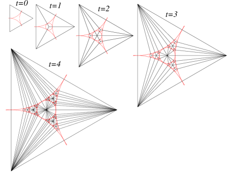
Figure 2: (colour online) The development of the 2D Apollonian network inside the interstice between three mutually touching disks, as the number of generations increases. In each picture, the network is overlaid on the underlying packing.

Figure 2 illustrates how the Apollonian packing can be used as a basis for a network, where each disk is a node in the network and nodes are connected if the corresponding disks are in contact. We shall call this contact network an Apollonian network. Of course, it has an infinite number of nodes. However, we shall generally consider the network properties after a finite number of generations in the development of the complete Apollonian network. From our analytical results we can quickly obtain the properties of the complete network by taking the limit of large $t$. However, the numerical results are necessarily limited to finite-sized networks.

Figure 2 also shows how the network evolves with the addition of new nodes at each generation. For each new disk added, three new interstices in the packing are created, that will be filled in the next generation. Equivalently, for each new node added, three new triangles are created in the network, into which nodes will be inserted in the next generation. Therefore,

$$\Delta n_{v}(t)=n_{v}(t)-n_{v}(t-1)=3\Delta n_{v}(t-1)\quad\ t>1,$$ (1)

where $n_{v}$ is the number of nodes in the network.

For the Apollonian packing of a circle, $n_{v}(0)=4$, and $\Delta n_{v}(1)=4$, if we treat the bounding circle on the same footing as the other three initial disks. It follows that

$$\Delta n_{v}(t)=4\,3^{t-1}\quad\ \hbox{and}\quad\ n_{v}(t)=2\left(3^{t}+1\right)$$ (2)

The addition of each new node leads to three new edges. Therefore,

$$\Delta n_{e}(t)=n_{e}(t)-n_{e}(t-1)=3\Delta n_{v}(t)=4\,3^{t},$$ (3)

where $n_{e}$ is the number of edges in the network. As $n_{e}(0)=6$

$$n_{e}(t)=2\,3^{t+1}$$ (4)

$p$, the fraction of all the possible pairs of nodes that are actually connected, is given by

$$p = {2n_{e}\over n_{v}(n_{v}-1)}={3^{t+1}\over(3^{t}+1)(3^{t}+1/2)}$$ (5)

$$\approx {1\over 3^{t-1}}\qquad\hbox{for large $t$}.$$

Therefore, the Apollonian network becomes increasingly sparse as its size increases. By contrast, the average degree tends to a limiting value:

$$\langle k\rangle = {2n_{e}\over n_{v}}={2\,3^{t+1}\over 3^{t}+1}$$ (6)

$$\approx 6\qquad\hbox{for large $t$}.$$

Surrounding each node $i$ are $k_{i}$ empty (i.e. not enclosing any nodes) triangles. As new nodes are added at the centre of all these triangles, $k_{i}$ new connections will be created. Therefore, at each step the degree of a node doubles, i.e.

$$k_{i}(t+1)=2k_{i}(t).$$ (7)

Such a rule expresses a preferential attachment Barabási and Albert (1999). The number of new connections is linearly proportional to the degree.

If $t_{c,i}$ is the step at which a node $i$ is created, $k(t_{c,i})=3$ and hence

$$k_{i}(t)=3\,2^{t-t_{c,i}}.$$ (8)

Therefore, $k$ can take a series of discrete values up to $k_{\rm max}=3\,2^{t}$. The fraction of the other nodes that the node with maximum degree connects to is given by

$${k_{\rm max}\over n_{v}-1} = {3\,2^{t}\over 2\,3^{t}+1}$$ (9)

$$\approx \left({2\over 3}\right)^{t-1}\qquad\hbox{for large $t$}$$

and is a decreasing fraction of the total as the size of the network increases. It follows that the degree distribution is given by

$$p(k)=\left\{\begin{array}[]{lc}{\displaystyle{n_{v}(0)\over n_{v}(t)}={2\over 3^{t}+1}}&\ \hbox{for}\ k=3\,2^{t},t_{c}=0\\ {\displaystyle{\Delta n_{v}(t_{c})\over n_{v}(t)}={2\,3^{t_{c}-1}\over 3^{t}+1}}&\ \hbox{for}\ k=3\,2^{t-t_{c}},t_{c}\geq 1\\ 0&\ \hbox{otherwise}\end{array}\right.$$ (10)

and that the cumulative degree distribution is

$$p_{\rm cum}(k)={3^{t_{c}}+1\over 3^{t}+1}.$$ (11)

Substituting for $t_{c}$ in this expression using $t_{c}=t-\log(k/3)/\log 2$ gives

$$p_{\rm cum}(k) = {3^{t}\left({k/3}\right)^{-\log 3/\log 2}+1\over 3^{t}+1}$$ (12)

$$\approx \left({k\over 3}\right)^{\textstyle-{\log 3\over\log 2}}\qquad\hbox{for large $t$}.$$

For a continuous degree distribution $p(k)\sim k^{-\gamma}$, $p_{\rm cum}(k)\sim k^{1-\gamma}$. Therefore, the Apollonian network is scale free and the exponent of the degree distribution is

$$\gamma=1+{\log 3\over\log 2}=2.585,$$ (13)

as already noted in Ref. Andrade et al., cond-mat/0406295. Apollonian networks hence provide a new model for spatial scale-free networks. Importantly, in contrast to other two-dimensional spatial scale-free networks Xulvi-Brunet and Sokolov (2002); Manna and Sen (2002); Sen and Manna (2003); Barthélemy (2003); Rozenfeld et al. (2002); Warren et al. (2002); ben Avraham et al. (2003); Herrmann et al. (2003), the Apollonian network can be embedded in a plane without any edges crossing. In Aste et al.’s classification scheme, they hence have a genus of zero Aste et al. (cond-mat/0408443).

Another important property of the network is the clustering, which provides a measure of the local structure within the network. The clustering coefficient of node $i$ is the probability that a pair of neighbours of $i$ are themselves connected.

$$c_{i}(t)={2n^{con}_{i}\over k_{i}(t)(k_{i}(t)-1)},$$ (14)

where $n^{con}_{i}$ is the number of connections between the neighbours of $i$. At each stage a ring of new connections passing through all the nodes connected to $i$ is generated. Therefore,

$$n^{con}_{i}(t)=\sum_{t^{\prime}=t_{c,i}}^{t}k_{i}(t^{\prime})=3\left(2^{t-t_{c,i}+1}-1\right),$$ (15)

and

$$c_{i}(t) = {2\left(2^{t-t_{c,i}+1}-1\right)\over 2^{t-t_{c,i}}\left(3\,2^{t-t_{c,i}}-1\right)}$$ (16)

$$\approx {1\over 3\,2^{t-t_{c,i}-2}}={4\over k_{i}(t)}\qquad\hbox{for $t\gg t_{c,i}$}.$$

Therefore, the clustering coefficient of a vertex shows the same inverse proportionality to the degree as has been obtained previously for other deterministic scale-free networks Dorogovtsev et al. (2002); Ravasz and Barabási (2003); Comellas et al. (2004). This feature has been taken to be a signature of a hierarchical structure to the network Ravasz and Barabási (2003); Barabási (2004), but recently has been shown to partially reflect disassortative correlations Soffer and Vázquez (cond-mat/040686). In the current networks this feature can also be interpreted in terms of spatial localization. For a low-degree node its neighbourhood only occupies a small local region in the packing, and thus would be expected to have strong clustering. By contrast, high-degree nodes have a more global character and are connected to well-separated parts of the packing, and so have low clustering.

The clustering coefficient for the whole graph can be defined in two ways. The first is a generalization of Eq. (14) to the whole graph, and is the probability that any pair of nodes with a common neighbour are themselves connected. Thus,

$$C_{1}={2\sum_{i}n_{i}^{con}\over\sum_{i}k_{i}(k_{i}-1)}.$$ (17)

The second definition of $C$ is as the average value of the local clustering coefficient, i.e.

$$C_{2}={1\over n_{v}}\sum_{i}c_{i}.$$ (18)

The difference between these two definitions is the relative weight given to nodes with different degree. High degree nodes make a larger contribution to $C_{1}$ because there will be more pairs of nodes that have a high-degree node as a common neighbour, whereas all nodes contribute equally to $C_{2}$. Typically, $C_{1}<C_{2}$ because, as is the case here, higher degree nodes tend to have lower values of $c_{i}$.

Substituting in and rearranging gives

$$C_{1} = {3^{t+1}-1\over 12\left(2^{2t-1}-3^{t-1}\right)}$$ (19)

$$\approx {1\over 2}\left({3\over 4}\right)^{t}.$$

The clustering coefficient goes down as the size of the Apollonian network increases. However when one compares $C$ to that for an Erdős-Renyi random graph Erdős and Rényi (1959, 1960) ($C_{\rm ER}=p$), one obtains

$${C_{1}\over C_{\rm ER}}\approx{1\over 6}\left({3\over 2}\right)^{2t}.$$ (20)

That is the Apollonian networks become increasingly more clustered than a random graph, as their size increases. $C_{2}$ can be evaluated numerically. As shown in Ref. Andrade et al., cond-mat/0406295, $C_{2}$ tends to a constant at large $t$ of value 0.828.

In Ref. Andrade et al., cond-mat/0406295, they also calculated the behaviour of $l_{\rm ave}$, the average number of steps on the shortest path between any two nodes. $l_{\rm ave}$ showed a small-world behaviour, scaling sub-logarithmically with network size Andrade et al. (cond-mat/0406295). The important role played by the larger disks in mediating these short paths is illustrated in Fig. 3. The vertex betweenness of a node is defined as the fraction of all the shortest paths that pass through that node. For $t=8$, 40% of these paths pass through the central disk in the packing (Fig. 2). Furthermore, the dependence of the vertex betweenness on the degree is not far from a power-law. This type of behaviour is common for scale-free networks Goh et al. (2002).

Figure 3: The dependence of the vertex betweenness on degree for the Apollonian network with $t=8$. There are points representing each disk and the line connects the average values for a given $k$.

Correlations in networks, particularly with respect to the degree, have been the subject of increasing interest Maslov and Sneppen (2002). This is partly because the behaviour of models defined on such networks have been often found to depend sensitively not only on the degree distribution, but also on how correlated the networks are Eguíluz and Klemm (2002); Boguñá et al. (2003); Vázquez and Weigt (2003); Echenique et al. (cond-mat/0406547). For example, $k_{\rm nn}(k)$, the average degree of the neighbours of nodes with degree $k$, should be independent of $k$ for an uncorrelated network.

We can calculate $k_{\rm nn}$ for the Apollonian network using Eq. (7) to work out how many connections are made at a particular step to nodes with a particular degree. Except for the initial disks, no disks created in the same generation, i.e. with the same degree, will be connected. All connections to nodes with higher degree are made at the generation step, and then connections to lower degree nodes are made at each subsequent step. This leads to the expression

$$k_{\rm nn}(k) = {1\over\Delta n_{v}(t_{c})k(t_{c},t)}\Bigg{(}$$ (21)

$$\sum_{t^{\prime}_{c}=0}^{t^{\prime}_{c}=t_{c}-1}\Delta n_{v}(t^{\prime}_{c})k(t^{\prime}_{c},t_{c}-1)k(t^{\prime}_{c},t)+$$

$$\sum_{t^{\prime}_{c}=t_{c}+1}^{t^{\prime}_{c}=t}\Delta n_{v}(t_{c})k(t_{c},t^{\prime}_{c}-1)k(t^{\prime}_{c},t)\Bigg{)}$$

for $k=3\,2^{t-t_{c}}$ and where $k(t_{c},t)$ is the degree of a node at generation $t$ that was created at generation $t_{c}$. The first sum corresponds to the connections made to nodes with higher degree (i.e. $t^{\prime}_{c}<t_{c}$) when the node was created at $t_{c}$, and the second sum to the connections made to the current lowest degree node at each step $t^{\prime}_{c}>t_{c}$. After substitution and evaluation of the sums, the above expression simplifies to

$$k_{\rm nn}(k)=9\left(4\over 3\right)^{t_{c}}-6+{3\over 2}(t-t_{c}).$$ (22)

After the initial generation step $k_{\rm nn}$ for a node increases linearly with age.

Figure 4: Comparison of $k_{\rm nn}/k_{\rm nn}^{\rm uncorr}$ for the 2D Apollonian network to that for randomized versions of the networks. Lines corresponding to different values of $t$ ($t=7$–15 and 7–8 for the Apollonian, and randomized networks, respectively) have been plotted to emphasize the universal form of this function for the Apollonian network.

Writing the above equation in terms of $k$ gives

$$k_{\rm nn}(k)=9\left({4\over 3}\right)^{t}\left({k\over 3}\right)^{\textstyle-{\log(4/3)\over\log 2}}-6+{3\log(k/3)\over 2\log 2}.$$ (23)

$k_{\rm nn}(k)$ is roughly a power law function of $k$ with exponent $-0.415$. The exponent is negative implying that the network is disassortative, i.e. nodes are more likely to be linked to nodes with dissimilar degree. When normalized by the expected value of $k$ for an uncorrelated network

$$k_{\rm nn}^{\rm uncorr}={\langle k^{2}\rangle\over\langle k\rangle}=6\left({4\over 3}\right)^{t}-3$$ (24)

$k_{\rm nn}(k)$ has a universal form independent of network size for large $t$ and small $k$. Namely,

$${k_{\rm nn}(k)\over k_{\rm nn}^{\rm uncorr}}\approx{3\over 2}\left({k\over 3}\right)^{\textstyle-{\log(4/3)\over\log 2}}.$$ (25)

This is illustrated in Figure 4. The upward curvature away from this power-law form at large $k$ is caused by the logarithmic term in $k$ in Equation (22).

It has been shown that disassortativity can often arise in networks where self-connections and multiple edges are excluded Park and Newman (2003). Therefore, $k_{\rm nn}$ was compared to that for random networks with the same degree distribution, which were prepared using the switching algorithm Maslov and Sneppen (2002); Milo et al. (cond-mat/0312028). The randomized networks also show disassortativity, but to a somewhat lesser degree (Fig. 4). The additional disassortativity arises because connections to the nodes with the same degree cannot occur in the Apollonian network (except for the initial disks).

In particular, as the nodes with $k=3$ are only connected to higher degree nodes, $k_{\rm nn}(3)$ is significantly higher than that for the randomized graph (Figure 4). By contrast, $k_{\rm nn}$ for the rest of the network is lower than that for the randomized graphs. This is also because of the lack of same-degree connections, as this gives the higher degree nodes many more connections to the most numerous $k=3$ nodes than for the randomized graphs.

Figure 5: Assortativity coefficients, $r_{k}$ and $r_{A}$, as a function of the number of generations $t$. The solid lines are for the 2D Apollonian network, and the dashed lines for randomized versions of these networks with the same degree distribution.

An assortativity coefficient $r$ has been proposed that measures the degree of (dis)assortativity of a property Newman (2002), and is defined as

$$r={\langle st\rangle_{e}-\langle s\rangle_{e}\langle t\rangle_{e}\over\langle st\rangle_{e,assort}-\langle s\rangle_{e}\langle t\rangle_{e}}.$$ (26)

where $s$ and $t$ correspond to the property of interest at either end of an edge, $e$ denotes that the averages are over all edges and assort that the average is for a perfectly assortative network. $r$ is therefore a measure of the correlations in the property compared to that for a perfectly assortative network. Disassortative networks have $r<0$.

It follows that the assortativity coefficient for the degree is given by

$$r_{k}={\langle k\rangle\langle k^{2}k_{\rm nn}(k)\rangle-\langle k^{2}\rangle^{2}\over\langle k\rangle\langle k^{3}\rangle-\langle k^{2}\rangle^{2}},$$ (27)

Expressions for the quantities in the above equation can be relatively easily obtained from the degree distribution. This gives

$$r_{k} = {3^{t}\left(2t-3+4\left({3\over 4}\right)^{t}\right)-2^{2t}\left(2-\left({3\over 4}\right)^{t}\right)^{2}\over{\displaystyle{3^{t}2^{t}\over 5}}\left(6-\left({3\over 8}\right)^{t}\right)-2^{2t}\left(2-\left({3\over 4}\right)^{t}\right)^{2}}$$ (28)

$$\approx -{10\over 3}\left({2\over 3}\right)^{t}\qquad\qquad\hbox{for large $t$.}$$

$r_{k}$ is always negative, indicating disassortativity. However, its magnitude goes to zero as the size of the network increases (Figure 5). This may seem surprising since $k_{\rm nn}$ always has a negative slope and has an effective functional form that is independent of size (Eq. (25)). However, the convergence of $r$ to zero is simply because the denominator corresponding to the correlations in a perfectly assortative network scales more rapidly with size than the numerator, i.e. as $6^{t}$ compared to $-4^{t}$ (Eq. (28)).

Figure 6: The best division of the 2D Apollonian packing into communities for $t=6$. The disks in the different communities have been displaced with respect to each other for clarity. The modularity $Q=0.5938$.

We also looked at the community structure of this network using the algorithm of Girvan and Newman Girvan and Newman (2002). It works by starting with the complete network and at each step removing the edge that has the maximum edge betweenness, where this quantity is recalculated after the removal of every edge and is defined as the fraction of all the shortest paths that pass through an edge. If there is more than one edge with the same maximum edge betweenness, they are all removed at the same step. Thus the network is progressively divided into $n_{v}$ communities. To decide which division of the network represents the best choice, the modularity $Q$ is calculated at each step, and the division of the system with maximum $Q$ is considered to be the best Newman and Girvan (2004). $Q$ is defined as the fraction of edges that are within the communities compared to that expected for a random graph with the same degree distribution.

The best division of the packing into communities is shown in Figure 6 for $t=6$ and has $Q=0.5938$. This value is comparable to some of the higher values found for networks considered previously Newman and Girvan (2004); Newman (2004). Interestingly, the Apollonian network’s combination of community structure and assortativity is in contrast to most of the other networks with high $Q$ which tend to be also strongly assortative. As expected the communities are spatially localized. As the algorithm only used topological information, this result implies that the spatial embedding of the network is clearly reflected in its topology.

Figure 7: A dendrogram showing the progressive division of the 2D Apollonian packing into communities for $t=6$ as those sets of edges with largest edge betweenness are removed. At right no edges have been removed and there is a single community of size $n_{v}$, whereas at left all edges have been removed and there are $n_{v}$ communities of size 1. The number of steps in which sets of edges have been removed increases linearly from right to left. In total 84 sets of edges were removed. The three-fold symmetry of the packing is retained throughout this process. The vertical dashed line indicates the set of communities with largest $Q$. The inset shows how $Q$ varies as the network is broken up into communities.

The algorithm for detecting communities described above cannot actually break the threefold symmetry of the packing. The best threefold symmetric division has the central disk as its own community. However, by assigning this disk to one of the adjacent communities, $Q$ improves from 0.5872 to 0.5938. We have also applied the faster algorithm described in Ref. Newman, 2004, however slightly lower values of $Q$ were obtained.

It is interesting to examine how the network is progressively broken into separate communities as more edges are removed. This can be represented by a dendrogram as in Figure 7, which shows the number of communities and their relationship at each step in the algorithm. Every time two sets of disks become disconnected, their corresponding lines split. The first 53 sets of edges removed only break the packing into two communities; instead the effect is to make the contact matrix sparser. Further removal of sets of edges then relatively quickly breaks the packing into a large number of communities.

It is evident that $Q$ has quite a broad maximum as a function of the number of communities. $Q$ is greater then 0.3 when there are between 6 and 88 communities. Given the self-similar nature of the packing, one would not expect there to be a strongly preferred size for the communities. Similarly, in the deterministic scale-free networks the hierarchical modularity means that there is no clearly preferred size for the modules at which the modularity is significantly enhanced Barabási (2004).

II.2 Other self-similar packings

The 2D Apollonian network is only one example of a space-filling self-similar packing. In a similar way to the last section, a detailed characterization of the topology of contact networks associated with other self-similar packings could be derived. However, here we do not wish to give such a comprehensive account, but to illustrate how some of the key features of these networks, particularly the exponent of the degree distribution, depend on the nature of the packing.

Firstly, we shall examine higher-dimensional Apollonian packings. The initial configuration that is directly equivalent to Figure 1 is to have touching hyperspheres at the corners of a $d$-dimensional simplex that is enclosed within and touching a larger hypersphere. The analysis of the last section is relatively easy to generalize to these cases.

As, now $n_{v}(0)=\Delta n_{v}(1)=(d+2)$ and $\Delta n_{v}(t)=(d+1)\Delta n_{v}(t-1)$ for $t>1$, it follows that

$$\Delta n_{v}(t)=(d+2)(d+1)^{t-1}$$ (29)

and

$$n_{v}(t)={(d+2)\over d}\left(\left(d+1\right)^{t}+d-1\right).$$ (30)

The higher dimensional equivalent of Eq. (7) is not so useful for calculating the degree distribution, for example for a 3-dimensional Apollonian packing $k_{i}(t+1)=3k_{i}(t)-4$. Instead, an alternative approach has to be used. Each new neighbour of a node $i$ creates $d$ new $d$-simplices involving $i$. In the next generation these $d$-simplices will be the sites for new nodes that are also neighbours of i. Therefore,

$$\Delta k_{i}(t) = k_{i}(t)-k_{i}(t-1)$$ (31)

$$= d\Delta k_{i}(t-1)\qquad{t>t_{c,i}+1}.$$

As $k_{i}(t_{c,i})=d+1$ and $\Delta k_{i}(t_{c,i}+1)=d+1$,

$$\Delta k_{i}(t)=(d+1)d^{t-t_{c,i}-1}$$ (32)

and

$$k_{i}(t)={d+1\over d-1}\left(d^{t-t_{c,i}}+d-2\right).$$ (33)

By an equivalent analysis to that for $d=2$ one can show that $p_{cum}(k)$ follows a power-law for large $t$ where

$$\gamma=1+{\log(d+1)\over\log d}.$$ (34)

Hence, the Apollonian networks associated with higher-dimensional packings are also scale-free networks. The exponent $\gamma$ decreases as the dimension of the Apollonian packing increases, tending to two in the limit of large $d$. This is noteworthy since the value of $\gamma$ can have significant effects on network properties Trusina et al. (2004).

By physical arguments it is easy to see that these higher-dimensional Apollonian networks will have very similar topological properties to the two-dimensional case that we have studied in detail. The networks will again be disassortative with respect to degree because of the lack of connections between nodes with the same degree. The hierarchical structure and the more localized character of the connections involving low-degree nodes will lead to a strong dependence of the clustering coefficient on degree. This spatial localization will also lead to strong community structure. Larger hyperspheres are also more likely to have a larger degree.

To illustrate how these conjectures can be backed up analytically, here we derive a general expression for the local clustering coefficient. We first need to calculate the number of connections between the neighbours of a node. On generation a node is surrounded by a $d$-dimensional simplex, and then at subsequent steps every new neighbour of a node contributes $d$ new connections to $n_{i}^{con}$. Hence,

$$n_{i}^{con}(t) = {d(d+1)\over 2}+\sum_{t^{\prime}=t_{c}+1}^{t}d\Delta k_{i}(t)$$ (35)

$$= {d+1\over d-1}d^{t-t_{c}+1}+{d(d+1)(d-3)\over 2(d-1).}$$

Substituting into Eq. 14 and taking limits gives:

$$c_{i}(t)\approx{2d\over k_{i}(t)}\qquad\hbox{for $t\gg t_{c,i}$}.$$ (36)

Again, the local clustering coefficient is inversely proportional to degree.

Figure 8: A space-filling bearing between two half planes. The pattern can be repeated to the left and to the right ad infinitum. In the numenclature of Refs. Herrmann et al., 1990; Manna and Herrmann, 1991; Manna and Viscek, 1991 this packing is from Family 1 and has base loop size 4 and $n=m=2$. The half-planes at the top and bottom can be considered as disks with infinite radius.

In the Apollonian packing of disks, the smallest loops in the contact network have size three, i.e. they are triangles. However, space-filling packings of disks are possible, where the smallest loops in the contact network are polygons with more than three sides. Examples, where the loops all have an even number of sides are of particular interest, since they can act as space-filling bearings, where all the disks can rotate at the same time without slip Herrmann et al. (1990); Oron and Herrmann (2000). An example of a space-filling bearings with ‘base loop size’ 4 and ‘$n=m$’. is shown in Figure 8. The procedures to construct such packings are more complex than for Apollonian packings and are described in detail in Refs. Herrmann et al., 1990; Manna and Herrmann, 1991; Manna and Viscek, 1991

Figure 9 illustrates how the contact network associated with this packing develops for a subset initially consisting of four touching disks. At each stage $m+1$ new nodes are produced for each empty quadrilateral, dividing the quadrilateral into a further $m+2$ new quadrilaterals to which new nodes will be added at the next generation.

Figure 9: (colour online) The development of the contact network for a subset of the packing in Fig. 8 initially consisting of four touching disks, one of which has infinite radius. The edges in the network connect the centres of the disks that touch. Those edges involving the infinitely large disk are parallel, but to emphasise that they do actually connect to the same node, a box has been added that enclosed the ends of these edges.

Assuming that there is one quadrilateral initially ($t=0$), the number of empty quadrilaterals after step $t$ is $(m+2)^{t}$. Hence,

$$\Delta n_{v}(t)=(m+1)(m+2)^{t-1}$$ (37)

and

$$n^{\prime}_{v}(t)=n_{v}(t)-n_{v}(0)=(m+2)^{t}-1.$$ (38)

We exclude the initial boundary disks in the above because they have slightly different properties from the rest of the disks in the iterative scheme. Besides, for sufficiently large $t$ their contribution is negligible.

Aside from the first step after a node is created, a node only gains new connections at every other step, because the new connections are added across alternating diagonals of the quadrilaterals.

$$k_{i}(t+2)=(m+2)k_{i}(t).$$ (39)

Therefore,

$$k_{i}(t)=2(m+2)^{(t-t_{c,i})/2}\quad\hbox{for $t-t_{c,i}$ even}.$$ (40)

In the same way as before this leads to

$$p_{cum}(k) = {(m+2)^{t}(k/2)^{-2}-1\over(m+2)^{t}-1}$$ (41)

$$\approx \left({k\over 2}\right)^{-2}\quad\hbox{for $t$ large}.$$

Hence $\gamma=-3$, independent of $m$. Unlike the Apollonian packings, $\Delta n_{v}$ and $k_{i}$ increase by the same factor $m+2$, and so this cancels. The power of two in the above equation arises, because this increase in $k_{i}$ occurs only at every other step. The situations is more complicated for the case $m\neq n$, because there are two sub-populations of disks, and the degree distribution of each sub-population obeys its own power law.

We should note that the contact networks for these space-filling bearings have no triangles, and so the clustering coefficient defined by Eq. (17) is zero. However, generalized clustering coefficients probing higher-order loops have been proposed. Clearly for these space-filling bearings the number of ‘squares’ (loops of length 4) will be significantly higher than for a random network, although we have not sought to quantify this.

The results in this section illustrate that the contact networks associated with other space-filling disk and hypersphere packings are also scale-free, but that the exponent of the degree distribution is not a universal constant but depends on the nature of the packing. We could have also considered other examples, such as scale-free bearings with base loop size greater than four Oron and Herrmann (2000) and non-Apollonian packings of spheres Mahmoodi Baram et al. (2004); Mahmoodi Baram and Herrmann (2004), and it is likely that these again show somewhat different behaviour.

III Spatial Properties

The 2D Apollonian packing is a well-known example of a fractal Mandelbrot (1983), and has many of the typical fractal properties. For example, inside every curvilinear triangle no matter how small the same pattern of disk packing reoccurs, i.e. it is self-similar. Similarly, the estimated total length of the circumferences of all the circles continues to increase as the resolution of the measurement increase. One of the most important properties of such a packing is its fractal dimension. To understand this quantity we need to define more carefully the set for which we wish to know the dimension. In the packing the disks are all considered to be open, that is the set of points associated with a disk $D_{i}$ contains all the points inside the disk boundary, but not the boundary itself. The residual set $R$ is then the points that are not part of any of the open disks in the packing, or more formally $R=U-\bigcup_{i=1}^{\infty}D_{i}$ where $U$ is the set that is being packed. $d_{F}$, the fractal dimension of $R$, is the quantity of interest.

$d_{F}$ must obey $1<d_{F}<2$. The upper bound is obvious, because, by virtue of the space-filling nature of the Apollonian packing, $R$ must have zero area. The lower bound follows from the fact that $\sum_{i=1}^{\infty}r_{i}=\infty$, where $r_{i}$ is the radius of disk $D_{i}$; i.e. the total length of the boundaries is infinite Wesler (1960). This result can most easily be visualized by projecting the boundaries of each disk onto a diameter of the circle bounding the region that is being packed. Points on this diameter are projected onto infinitely often. These bounds imply the dimension of $R$ must be fractional, and hence the packing is fractal.

So far, no analytic formula for the value of the fractal dimension for the 2D Apollonian packing has been obtained, but instead its numerical value has beens estimated with increasing precision Hirst (1967); Larman (1967); Boyd (1973, 1982); Manna and Herrmann (1991); Thomas and Dhar (1994). Its value is 1.3057. It has been suggested that the fractal dimension of the Apollonian packing is the minimum for any space-filling disk packing Melzak (1966a), because at each step of the generating process the disk with maximum possible radius is inserted into each curvilinear triangle, thus maximizing the area of the region that must be outside of the residual set. The fractal dimensions found for 2D space-filling bearings are consistent with this assertion Manna and Herrmann (1991); Oron and Herrmann (2000); all have larger values than that for the Apollonian packing with the largest found being 1.803. In fact, as pointed out by Melzak, it is easy to generate a disk packing with dimension arbitrarily close to 2 Melzak (1966a). If each disk in the Apollonian packing in Figure 1 is replaced by a suitably scaled image of the whole Apollonian packing, a new packing is obtained with higher fractal dimension. If this process is repeated ad infinitum, a disk packing with a fractal dimension of 2 is eventually obtained.

For space-filling packings of $d$-dimensional hyperspheres, there are similar limits for the fractal dimension, namely $d-1<d_{F}<d$. The only calculations have been for three dimensions. The Apollonian packing has $d_{F}=2.4739$ Borkovec et al. (1994), and the values for space-filling bearings are again larger Mahmoodi Baram and Herrmann (2004).

The fractal dimension is of particular interest here, because it provides a means to characterize the properties of the disk areas. Melzak introduced the exponent of a packing, $d_{r}$, defining it as the minimum value of $s$ for which $\sum_{i=1}^{\infty}r_{i}^{s}$ no longer diverges. It was proved by Boyd that for the Apollonian packing that $d_{F}=d_{r}$ Boyd (1973). To examine the divergence properties of this sum we can replace the sum by an integral, because the divergence is controlled by the disks with small radii, for which the distribution of radii is quasicontinuous. As this distribution follows a power law, $p(r)\sim r^{-\beta}$ Melzak (1966b), we have

$$\sum_{i=1}^{\infty}r_{i}^{s} \approx \int^{r_{\rm max}}_{0}r^{s}p(r)dr\sim\int^{r_{\rm max}}_{0}r^{s-\beta}$$

$$= \left[{r^{s+1-\beta}\over s+1-\beta}\right]^{r_{\rm max}}_{0}$$

$$= \infty\qquad\hbox{if }s<\beta-1$$

Hence, $d_{F}=d_{r}=\beta-1$. This allows the fractal dimension to be determined from the exponent of the numerically obtained $p(r)$ Boyd (1982). It follows that the area distribution is given by $p(A)=A^{-(1+d_{F}/2)}$ for the 2D case and more generally for packings of $d$-dimensional hyperspheres the volume distribution

$$p(V)=V^{-(1+d_{F}/d)}\approx V^{-2}\qquad\hbox{for large $d$}.$$ (43)

Given the bounds for $d_{F}$ the exponent must lie between $2-1/d$ and $2$.

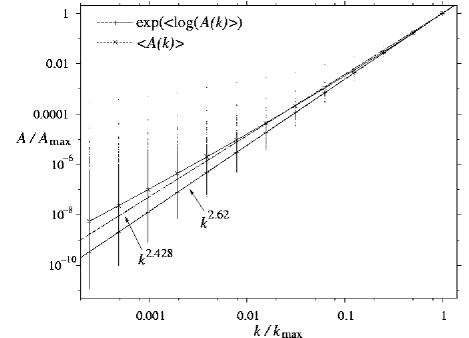
Figure 10: The correlation of disk area with degree for the 2D Apollonian packing (iterated to 15 generations). There is a dot representing each disk. The two lines with data points represent the average value of the area for a given degree, and correspond to both the normal and logarithmic averages. In addition lines corresponding to $(k/k_{\rm max})^{2.62}$ and $(k/k_{\rm max})^{2.428}$ have been plotted for comparison.

One of the areas that is of most interest to us, and which is particularly relevant to the energy landscape networks, is the connection between the spatial properties of the Apollonian packings and the topological properties of the Apollonian networks. In Figure 10 we show the correlation between the disk area and degree. As expected, the larger disks generally have a larger degree. However, for a given $k$ there is a wide variety of disk areas. The largest disks are associated with the crevices between the initial disks, whereas the smallest disks are obtained by following a spiral pathway in the network where each disk along the path is connected to one circle in each of the three previous generations.

More specifically, the logarithmic average of the disk area for a given $k$ closely follows a power-law. Assuming $A(k)\sim k^{\alpha}$ and using the identity $p(A)dA/dk=p(k)$ one can show that $\alpha=2(\gamma-1)/(\beta-1)$. For the 2D Apollonian network this leads to the prediction $\alpha=2.428$. A line with this exponent is plotted for comparison in Fig. 10, and broadly follows the average $\langle A(k)\rangle$. By contrast, the average $\exp(\langle\log A(k)\rangle)$ has an exponent of 2.62.

Although the correlations associated with the degree are most commonly studied, one can use Eq. (26) to define an assortativity coefficient with respect to any property. Here, we examine the correlations in the areas of touching disks. From the behaviour of $r_{A}$ in Fig. 5 one can see that there is some slight disassortativity, but much weaker than for the degree and with little difference from that for the randomized graphs. However, if there was no variation in the areas of the disks with a given $k$, (i.e. all the areas exactly obeyed the power-law dependence of $k$ that characterizes the average) then $r_{A}$ and $r_{k}$ would be very similar. Instead, because there is such a large scatter around the average values—over seven decades for the $k=3$ disks in Fig. 10—the effect of the lack of connections between nodes with the same degree only weakly carries over to disks with similar areas.

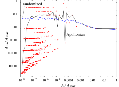
Figure 11: (colour online) The average area of the disks that a touch a disk against the area of that disk. The lines are binned averages for the Apollonian networks with $t=8$ and a randomized version of that network. There is a data point for each disk in the Apollonian packing. Those represented by a cross are in contact with at least one of the three initial disks, and those represented by a diamond are not.

These effects can be examined in more detail by calculating $A_{\rm nn}$, the average area of the neighbours of a disk. Weak disassortativity is evident over the majority of the range of areas, except for the smallest disks which show strong assortativity (Figure 11). This latter effect is simply because the smaller disks in the last generation are connected to the smaller disks in the previous generations, as with the spiral pathways mentioned above. Interestingly, Fig. 11 clearly divides the disks into two sets depending on whether they are in contact with one of the initial disks, and this is the source of the large fluctuations in the average value of $A_{nn}$ at intermediate values of the disk area.

Figure 12: (a) The cumulative size distribution of the disks for an Apollonian packing after a finite number of generations. The lines are labelled by their value of $t$, and an additional straight line with the exponent expected for the complete Apollonian packing has been added for comparison. (b) The cumulative degree distribution for a series of Apollonian network where only disks with radii at least $x$% of that of the largest disk contribute. The lines are labelled by their value of $x$, and additional straight lines have been added for comparison, one of which has the exponent expected for the complete Apollonian packing.

IV Discussion

Our main motivation for studying the properties of the Apollonian networks is their potential to act as a useful model for the energy landscape networks. However, there is one major difference between the two systems. The Apollonian packings contain an infinite number of disks or hyperspheres, whereas configuration space is divided up into a finite number of basins, albeit a number that is an exponentially increasing function of the number of atoms in the system Stillinger and Weber (1982); Doye and Wales (2002).

There are two ways of creating a finite network from the complete Apollonian network. The first is to consider the network produced after a finite number of generations, and is the one we have mainly used so far. The second is to consider the network containing only disks that are larger than a certain size. The wide distribution of areas for a given $k$ in Fig. 10 indicates that their could potentially be significant differences. We know that the first will have a scale-free degree distribution, and the second a power-law distribution of radii up to their respective cutoffs, but what about the other way round.

In Figure 12(a) the distribution of radii is shown after different numbers of generations. These distributions approximately follow the expected power law for intermediate values of the radii, but this range becomes increasingly small as $t$ decreases. Furthermore, at small $r$ the lines curve away from this power law, because the finite packings only contain a small fraction of the total number of disks in the complete packing with that $r$.

The degree distributions for networks generated using a size cutoff are shown in Fig. 12(b). The distributions still follow a power-law, and are actually smoother, since $k$ is no longer just restricted to the values given by Eq. 8. However, the exponent is slightly smaller than predicted by Eq. (13). The effect of the size cutoff is to only include the larger disks from the later generations, which are in turn more likely to be connected to the larger higher degree disks. For example, for a radius cutoff at 0.0001% of that of the largest disk, the first disks below the size cutoff occurred in the $13^{\rm th}$ generation, and the last disks included were in the $706^{\rm th}$ generation.

Preliminary results for the basin area distributions for the small clusters used to generate the energy landscape networks Mas look quite like Fig. 12(a) suggesting that Apollonian networks with a given number of generations are the more appropriate finite version for comparison with these systems. Furthermore, there are then some useful parallels between $t$ and $N$, the number of atoms in the cluster. For example, the number of minima increases exponentially with $N$ and the number of disks/hyperspheres in the Apollonian networks have a similar dependence on $t$ (Eqs. 2 and 30). Similarly, as either $t$ or $N$ increase, both types of networks become increasingly sparse (Eq. 5), have a smaller absolute value for the clustering coefficient $C_{1}$ (Eq. 17), but a larger value relative to that for an Erdős-Renyi random graph (Eq. 20) Doye (2002); Doye and Massen .

Other similarities between the two types of network include features that are quite common for scale-free networks, such as the dependence of vertex betweenness and local clustering coefficient on degree. Both are also disassortative Doye and Massen , however, there is greater community structure in the Apollonian networks Mas . There are also similar relationships between the topological and spatial properties, such as for the dependence of disk or basin areas on $k$ Mas .

One of the interesting possibilities raised by the current study is the signature of the scale-free topology of the Apollonian network in the power-law behaviour of the disk areas. Currently, mapping out the whole network of connections between minima on an energy landscape is only feasible for systems of very small size. Neither are there methods available to construct a statistical representation of the whole network from a finite sample. Therefore, it is hard to test how generic is the scale-free behaviour observed for the clusters. However, the distribution of the hyperareas of the basins of attraction on a energy landscape is a static quantity that could potentially be statistically sampled for a system of arbitrary size Doye et al. (1998). If this distribution exhibited a power law with exponent $-2$, (Eq. (43)), it would strongly suggest that underlying this was a scale-free energy landscape network, as for the Lennard-Jones clusters. Preliminary calculations indicate that this is the case Mas .

V Conclusions

We have analysed the properties of the contact networks of space-filling packings of disks and hyperspheres, focussing on the Apollonian packing of two-dimensional disks. Their topological properties include a scale-free degree distribution whose exponent depends on the nature of the packing, high overall clustering, a local clustering coefficient that is inversely proportional to degree, disassortativity by degree and strong community structure.

These networks have many similarities to other deterministic scale-free networks introduced and analysed recently Barabási and Ravasz (2001); Dorogovtsev et al. (2002); Jung et al. (2002); Ravasz and Barabási (2003); Comellas et al. (2004), but with the additional feature that they have a well-defined spatial embedding. For this reason, we have suggested that these packings provide a useful model spatial scale-free network that may help to explain the properties of energy landscapes and the associated scale-free network of connected minima. In particular, the scale-free topology of the Apollonian networks reflects the power-law distribution of disk sizes. Similarly, configuration space can be divided up into basins of attraction that surround the minima on the energy landscape. A similar power-law distribution for the hyperareas of these basins might thus provide an explanation for the pattern of connections between the minima.

References

- Watts and Strogatz (1998) D. J. Watts and S. H. Strogatz, Nature 393, 440 (1998).
- Strogatz (2001) S. H. Strogatz, Nature 410, 268 (2001).
- Albert and Barabási (2002) R. Albert and A. L. Barabási, Rev. Mod. Phys. 74, 47 (2002).
- Barabási (2002) A. L. Barabási, Linked: The New Science of Networks (Perseus Publishing, Cambridge, 2002).
- Bornholdt and Schuster (2003) S. Bornholdt and H. G. Schuster, eds., Handbook of Graphs and Networks: From the Genome to the Internet (Wiley-VCH, Weinheim, 2003).
- Dorogovtsev and Mendes (2003) S. N. Dorogovtsev and J. F. F. Mendes, Evolution of Networks: From Biological Nets to the Internet and WWW (Oxford University Press, Oxford, 2003).
- Newman (2003) M. E. J. Newman, SIAM Rev. 45, 167 (2003).
- Hughes et al. (2003) D. Hughes, M. Paczuski, R. O. Dendy, P. Helander, and K. G. McClements, Phys. Rev. Lett. 90, 131101 (2003).
- Baiesi and Paczuski (2004) M. Baiesi and M. Paczuski, Phys. Rev. E 69, 066106 (2004).
- Albert et al. (1999) R. Albert, H. Jeong, and A. L. Barabási, Nature 401, 130 (1999).
- Jeong et al. (2000) H. Jeong, B. Tombor, R. Albert, Z. N. Oltvai, and A. L. Barabási, Nature 407, 651 (2000).
- Jeong et al. (2001) H. Jeong, S. Mason, A. L. Barabási, and Z. N. Oltvai, Nature 411, 41 (2001).
- Dunne et al. (2002) J. A. Dunne, R. J. Williams, and N. D. Martinez, Proc. Natl. Acad. Sci. USA 99, 12917 (2002).
- Liljeros et al. (2001) F. Liljeros, C. R. Edling, L. A. N. Amaral, H. E. Stanley, and Y. Aberg, Nature 411, 907 (2001).
- Barabási and Albert (1999) A. L. Barabási and R. Albert, Science 286, 509 (1999).
- Maslov and Sneppen (2002) S. Maslov and K. Sneppen, Science 296, 910 (2002).
- Girvan and Newman (2002) M. Girvan and M. E. J. Newman, Proc. Natl. Acad. Sci. USA 99, 7821 (2002).
- Gastner and Newman (cond-mat/0407680) M. T. Gastner and M. E. J. Newman (cond-mat/0407680).
- S.-H. et al. (2002) Y. S.-H., H. Jeong, and A. L. Barabási, Proc. Natl. Acad. Sci. USA 99, 13382 (2002).
- Manna and Sen (2002) S. S. Manna and P. Sen, Phys. Rev. E 66, 066114 (2002).
- Xulvi-Brunet and Sokolov (2002) R. Xulvi-Brunet and I. M. Sokolov, Phys. Rev. E 66, 026118 (2002).
- Sen and Manna (2003) P. Sen and S. S. Manna, Phys. Rev. E 68, 026104 (2003).
- Barthélemy (2003) M. Barthélemy, Europhys. Lett. 63, 915 (2003).
- Rozenfeld et al. (2002) A. F. Rozenfeld, R. Cohen, D. ben Avraham, and S. Havlin, Phys. Rev. Lett. 89, 218701 (2002).
- Warren et al. (2002) C. P. Warren, L. M. Sander, and I. M. Sokolov, Phys. Rev. E 66, 056105 (2002).
- ben Avraham et al. (2003) D. ben Avraham, A. F. Rozenfeld, R. Cohen, and S. Havlin, Physica A 330, 107 (2003).
- Herrmann et al. (2003) C. Herrmann, M. Barthélemy, and P. Provero, Phys. Rev. E 68, 026128 (2003).
- Doye (2002) J. P. K. Doye, Phys. Rev. Lett. 88, 238701 (2002).
- (29) J. P. K. Doye and C. P. Massen, in preparation.
- Stillinger and Weber (1984) F. H. Stillinger and T. A. Weber, Science 225, 983 (1984).
- Rao and Caflisch (2004) F. Rao and A. Caflisch, J. Mol. Biol. 342, 299 (2004).
- Doye et al. (1998) J. P. K. Doye, D. J. Wales, and M. A. Miller, J. Chem. Phys. 109, 8143 (1998).
- Andrade et al. (cond-mat/0406295) J. S. Andrade, H. J. Herrmann, R. F. S. Andrade, and L. R. da Silva (cond-mat/0406295).
- Soddy (1936) F. Soddy, Nature 137, 1021 (1936).
- Aste et al. (cond-mat/0408443) T. Aste, T. Di Matteo, and S. T. Hyde, Physica A, in press (cond-mat/0408443).
- Ravasz and Barabási (2003) E. Ravasz and A. L. Barabási, Phys. Rev. E 67, 026112 (2003).
- Dorogovtsev et al. (2002) S. N. Dorogovtsev, A. V. Goltsev, and J. F. F. Mendes, Phys. Rev. E 65, 066122 (2002).
- Comellas et al. (2004) F. Comellas, G. Fertin, and A. Raspaud, Phys. Rev. E 69, 037104 (2004).
- Barabási (2004) A. L. Barabási, Nature Reviews Genetics 5, 101 (2004).
- Soffer and Vázquez (cond-mat/040686) S. N. Soffer and A. Vázquez (cond-mat/040686).
- Erdős and Rényi (1959) P. Erdős and A. Rényi, Publ. Math. Debrecen 6, 290 (1959).
- Erdős and Rényi (1960) P. Erdős and A. Rényi, Magyar Tud. Akad. Mat. Kutató Int. Közl. 5, 17 (1960).
- Goh et al. (2002) K.-I. Goh, E. Oh, H. Jeong, B. Kahng, and D. Kim, Proc. Natl. Acad. Sci. USA 99, 12583 (2002).
- Eguíluz and Klemm (2002) V. M. Eguíluz and K. Klemm, Phys. Rev. Lett. 89, 108701 (2002).
- Boguñá et al. (2003) M. Boguñá, R. Pastor-Satorras, and A. Vespignani, Phys. Rev. Lett. 90, 028701 (2003).
- Echenique et al. (cond-mat/0406547) P. Echenique, J. Gómez-Gardenes, Y. Moreno, and A. Vázquez (cond-mat/0406547).
- Vázquez and Weigt (2003) A. Vázquez and M. Weigt, Phys. Rev. E 67, 027101 (2003).
- Park and Newman (2003) J. Park and M. E. J. Newman, Phys. Rev. E 68, 026112 (2003).
- Milo et al. (cond-mat/0312028) R. Milo, N. Kashtan, S. Itzkovitz, M. E. J. Newman, and U. Alon, Phys. Rev. E, in press (cond-mat/0312028).
- Newman (2002) M. E. J. Newman, Phys. Rev. Lett. 89, 208701 (2002).
- Newman and Girvan (2004) M. E. J. Newman and M. Girvan, Phys. Rev. E 69, 026113 (2004).
- Newman (2004) M. E. J. Newman, Phys. Rev. E 69, 066133 (2004).
- Trusina et al. (2004) A. Trusina, S. Maslov, P. Minnhagen, and K. Sneppen, Phys. Rev. Lett. 92, 178702 (2004).
- Manna and Herrmann (1991) S. S. Manna and H. J. Herrmann, J. Phys. A 24, L481 (1991).
- Herrmann et al. (1990) H. J. Herrmann, G. Mantica, and D. Bessis, Phys. Rev. Lett. 65, 3223 (1990).
- Manna and Viscek (1991) S. S. Manna and T. Viscek, J. Stat. Phys. 64, 525 (1991).
- Oron and Herrmann (2000) G. Oron and H. J. Herrmann, J. Phys. A 33, 1417 (2000).
- Mahmoodi Baram et al. (2004) R. Mahmoodi Baram, H. J. Herrmann, and N. Rivier, Phys. Rev. Lett. 92, 044301 (2004).
- Mahmoodi Baram and Herrmann (2004) R. Mahmoodi Baram and H. J. Herrmann, Fractals 12, 293 (2004).
- Mandelbrot (1983) B. B. Mandelbrot, The Fractal Geometry of Nature (W. H. Freeman, New York, 1983).
- Wesler (1960) O. Wesler, Proc. Amer. Math. Soc. 11, 324 (1960).
- Thomas and Dhar (1994) P. B. Thomas and D. Dhar, J. Phys. A 27, 2257 (1994).
- Hirst (1967) K. E. Hirst, J. Lond. Math. Soc. 42, 281 (1967).
- Larman (1967) D. G. Larman, J. Lond. Math. Soc. 42, 292 (1967).
- Boyd (1973) D. W. Boyd, Mathematika 20, 170 (1973).
- Boyd (1982) D. W. Boyd, Math. Comput. 39, 249 (1982).
- Melzak (1966a) Z. A. Melzak, Canad. J. Math. 16, 838 (1966a).
- Borkovec et al. (1994) M. Borkovec, W. De Paris, and R. Peikert, Fractals 2, 521 (1994).
- Melzak (1966b) Z. A. Melzak, Math. Comput. 16, 838 (1966b).
- Stillinger and Weber (1982) F. H. Stillinger and T. A. Weber, Phys. Rev. A 25, 978 (1982).
- Doye and Wales (2002) J. P. K. Doye and D. J. Wales, J. Chem. Phys. 116, 3777 (2002).
- (72) C. P. Massen and J. P. K. Doye, unpublished.
- Barabási and Ravasz (2001) A. L. Barabási and E. Ravasz, Physica A 299, 559 (2001).
- Jung et al. (2002) S. Jung, S. Kim, and B. Kahng, Phys. Rev. E 65, 056101 (2002).