The instanton vacuum of generalized $CP^{N-1}$ models

Abstract

It has recently been pointed out that the existence of massless chiral edge excitations has important strong coupling consequences for the topological concept of an instanton vacuum. In the first part of this paper we elaborate on the effective action for “edge excitations” in the Grassmannian $U(m+n)/U(m)\times U(n)$ non-linear sigma model in the presence of the $\theta$ term. This effective action contains complete information on the low energy dynamics of the system and defines the renormalization of the theory in an unambiguous manner. In the second part of this paper we revisit the instanton methodology and embark on the non-perturbative aspects of the renormalization group including the anomalous dimension of mass terms. The non-perturbative corrections to both the $\beta$ and $\gamma$ functions are obtained while avoiding the technical difficulties associated with the idea of constrained instantons. In the final part of this paper we present the detailed consequences of our computations for the quantum critical behavior at $\theta=\pi$. In the range $0\leq m,n\lesssim 1$ we find quantum critical behavior with exponents that vary continuously with varying values of $m$ and $n$. Our results display a smooth interpolation between the physically very different theories with $m=n=0$ (disordered electron gas, quantum Hall effect) and $m=n=1$ ($O(3)$ non-linear sigma model, quantum spin chains) respectively, in which cases the critical indices are known from other sources. We conclude that instantons provide not only a qualitative assessment of the singularity structure of the theory as a whole, but also remarkably accurate numerical estimates of the quantum critical details (critical indices) at $\theta=\pi$ for varying values of $m$ and $n$.

1 Introduction

1.1 Super universality

The quantum Hall effect has remained one of the most beautiful and outstanding experimental realizations of the instanton vacuum concept in non-linear sigma models [1, 2]. Although originally introduced in the context of Anderson (de-)localization in strong magnetic fields [3, 4], the topological ideas in quantum field theory have mainly been extended in recent years to include a range of physical phenomena and applications that are much richer and broader than what was previously anticipated. What remarkably emerges is that the aforementioned topological concepts retain their significance also when the Coulomb interaction between the disordered electrons is taken into account [5]. A detailed understanding of interaction effects is vitally important not only for conducting experiments on quantum criticality of the plateau transitions [6, 7], but also for the long standing quest for a unified action that incorporates the low energy dynamics of both the integral and fractional quantum Hall states [9, 10, 11, 12, 13].

Perhaps the most profound advancement in the field has been the idea which says that the instanton vacuum generally displays massless chiral edge excitations [11, 14, 15]. These provide the resolution of the many strong coupling problems that historically have been associated with the instanton vacuum concept in scale invariant theories [16, 17, 18]. The physical significance of the edge is most clearly demonstrated by the fact that the instanton vacuum theory, unlike the phenomenological approaches to the fractional quantum Hall effect based on Chern Simons gauge theory [19], can be used to derive from first principles the complete Luttinger liquid theory of edge excitations in disordered abelian quantum Hall systems [11]. Along with the physics of the edge came the important general statement which says that the fundamental features of the quantum Hall effect should all be regarded as super universal features of the topological concept of an instanton vacuum, i.e. independent of the number of field components in the theory [14].

Super universality includes not only the appearance of massless chiral edge excitations but also the existence of gapless bulk excitations at $\theta=\pi$ in general as well as the dynamic generation of robust topological quantum numbers that explain the precision and observability of the quantum Hall effect [14, 15]. Moreover, the previously unrecognized concept of super universality provides the basic answer to the historical controversies on such fundamental issues as the quantization of topological charge, the exact significance of having discrete topological sectors in the theory, the precise meaning of instantons and instanton gases [16, 17], the validity of the replica method [20] etc. etc. One can now state that many of these historical problems arose because of a complete lack of any physical assessment of the theory, both in general and in more specific cases such as the exactly solvable large $N$ expansion of the $CP^{N-1}$ model.

1.2 The background field methodology

In 1987, one of the authors introduced a renormalization group scheme in replica field theory (non-linear sigma model) that was specifically designed for the purpose of extracting the non-perturbative features of the quantum Hall regime from the instanton angle $\theta$ [21, 22]. This procedure was motivated, to a large extend, by the Kubo formalism for the conductances which, in turn, has a natural translation in quantum field theory, namely the background field methodology.

Generally speaking, the background field procedure expresses the renormalization of the theory in terms of the response of the system to a change in the boundary conditions. It has turned out that this procedure has a quite general significance in asymptotically free field theory that is not limited to replica limits and condensed matter applications alone. It actually provides a general, conceptual framework for the understanding of the strong coupling aspects of the theory that otherwise remain inaccessible. For example, such non-perturbative features like dynamic mass generation are in one-to-one correspondence with the renormalized parameters of the theory since they are, by construction, a probe for the sensitivity of the system to a change in the boundary conditions.

The background field procedure has been particularly illuminating as far as the perturbative aspects of the renormalization group is concerned. First of all, it is the appropriate generalization of Thouless’ ideas on localization [23], indicating that the physical objectives in condensed matter theory and those in asymptotically free field theory are in many ways the same. Secondly, it provides certain technical advantages in actual computations and yields more relevant results. For example, it has led to an exact solution (in the context of an $\epsilon$ expansion) of the the AC conductivity in the mobility edge problem or metal-insulator problem in $2+\epsilon$ dimensions [13]. The physical significance of these results is not limited, once more, to the theory in the replica limit alone. They teach us something quite general about the statistical mechanics of the Goldstone phase in low dimensions.

1.3 The strong coupling problem

With hindsight one can say that the background field procedure [22], as it stood for a very long time, did not provide the complete conceptual framework that is necessary for general understanding of the quantum Hall effect or, for that matter, the instanton vacuum concept in quantum field theory. Unlike the conventional theory where the precise details of the “edge” do not play any significant role, in the presence of the instanton parameter $\theta$ the choice in the boundary conditions suddenly becomes an all important conceptual issue that is directly related to the definition of a fundamental quantity in the theory, the Hall conductance.

The physical significance of boundary conditions in this problem has been an annoying and long standing puzzle that has fundamentally complicated the development of a microscopic theory of the quantum Hall effect [1]. In most places in the literature this problem has been ignored altogether [16, 17, 18]. In several other cases, however, it has led to a mishandling of the theory [24].

The discovery of super universality in non-linear sigma models [25] has provided the physical clarity that previously was lacking. The existence of massless chiral edge excitations, well known in studies of quantum Hall systems, implies that the instanton vacuum concept generally supports distinctly different modes of excitation, those describing the bulk of the system and those associated with the edge. It has turned out that each of these modes has a fundamentally different topological significance, and a completely different behavior under the action of the renormalization group.

The existence of massless chiral edge excitations forces one to develop a general understanding of the instanton vacuum concept that is in many ways very different from the conventional ideas and expectations in the field. It turns out that most of the physics of the problem emerges by asking how the two dimensional bulk modes and one dimensional edge modes can be separated and studied individually. At the same time, a distinction ought to be made between the physical observables that are defined by the bulk of the system and those that are associated with the edge.

1.3.1 Effective action for the edge modes

The remarkable thing about the problem with edge modes is that it automatically provides all the fundamental quantities and topological concepts that are necessary to describe and understand the low energy dynamics of the system. Much of the resolution to the problem resides in the fact that the theory can generally be written in terms of bulk field variables that are embedded in a background of the topologically different edge field configurations. This permits one to formulate an effective action for the edge modes, obtained by formally eliminating all the bulk degrees of freedom from the theory [14, 15, 25]. It now turns out that the effective action procedure for the edge field variables proceeds along exactly the same lines as the background field methodology [22] that was previously introduced for entirely different physical reasons! This remarkable coincidence has a deep physical significance and far reaching physical consequences. In fact, the many different aspects of the problem (Kubo formulae, renormalization, edge currents etc.) as well as the various disconnected pieces of the puzzle (boundary conditions, quantization of topological charge, quantum Hall effect etc.) now become simultaneously important. They all come together as fundamental and distinctly different aspects of a single new concept in the problem that has emerged from the instanton vacuum itself, the effective action for the massless chiral edge excitations [14, 15, 25].

1.3.2 The quantum Hall effect

The effective action for massless edge excitations has direct consequences for the strong coupling behavior of the theory that previously remained concealed. It essentially tells us how the instanton vacuum dynamically generates the aforementioned super universal features of the quantum Hall effect, in the limit of large distances.

The large $N$ expansion of the $CP^{N-1}$ model can be used as an illuminating and exactly solvable example that sets the stage for the super universality concept in asymptotically free field theory [25]. The most significant quantities of the theory are the renormalization group $\beta$ functions for the response parameters $\sigma_{xx}$ and $\sigma_{xy}$ that appear in the effective action for massless chiral edge excitations, (see also Fig. 1)

$$\frac{d\sigma_{xx}}{d\ln\mu}=\beta_{\sigma}(\sigma_{xx},\sigma_{xy})$$ (1)

$$\frac{d\sigma_{xy}}{d\ln\mu}=\beta_{\theta}(\sigma_{xx},\sigma_{xy}).$$ (2)

Here, the parameters $\sigma_{xx}$ and $\sigma_{xy}$ are precisely analogous to the Kubo formulae for longitudinal conductance and Hall conductance in quantum Hall systems. They stand for the (inverse) coupling constant and $\theta/2\pi$ respectively, both of which appear as running parameters in quantum field theory.

The infrared stable fixed points in Fig. 1, located at integer values of $\sigma_{xy}$, indicate that the Hall conductance is robustly quantized with corrections that are exponentially small in the size of the system [25]. The unstable fixed points at half-integer values of $\sigma_{xy}$ or $\theta=\pi$ indicate that the large $N$ system develops a gapless phase or a continuously divergent correlation length $\xi$ with a critical exponent $\nu$ equal to $1/2$ [25],

$$\xi\propto|\theta-\pi|^{-1/2}.$$ (3)

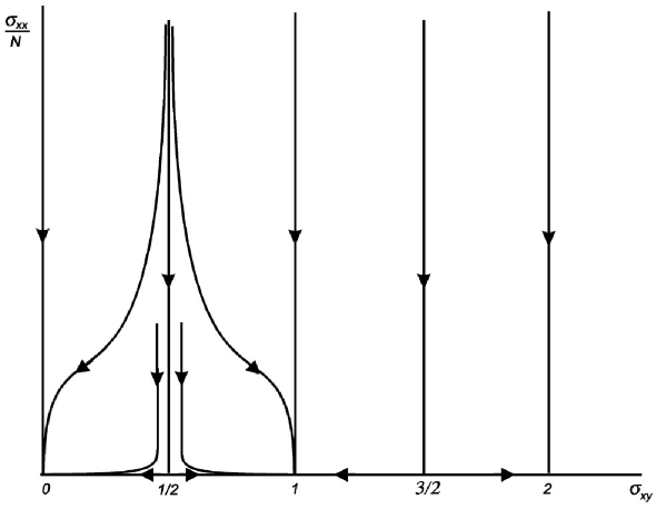
Figure 1: Large N renormalization group flow diagram for $\sigma_{xx}/N$ and the Hall conductance $\sigma_{xy}=\theta/2\pi$. The arrows indicate the direction toward the infrared.

1.4 The large $N$ expansion

One of the most impressive features of the large $N$ expansion is that it is exactly solvable for all values of $\theta$. This is unlike the $O(3)$ non-linear sigma model, for example, which is known to be integrable for $\theta=0$ and $\pi$ only and the exact information that can be extracted is rather limited [26]. Nevertheless, both cases appear as outstanding limiting examples in the more general context of replica field theory or, equivalently, the Grassmannian $U(m+n)/U(m)\times U(n)$ non-linear sigma model. This Grassmannian manifold is a generalization of the $CP^{N-1}$ manifold that describes, as is well known, the Anderson localization problem in strong magnetic fields [4].

It is extremely important to know, however, that none of the super universal features of the instanton vacuum where previously known to exist, neither in the historical papers on the large $N$ expansion [16, 17, 18, 27] nor in the intensively studied $O(3)$ case [26]. In fact, the large $N$ expansion, as it now stands, is in many ways an onslaught on the many incorrect ideas and expectations in the field that are based on the historical papers on the subject [16, 17, 27]. These historical papers are not only in conflict with the basic features of the quantum Hall effect, but also present a fundamentally incorrect albeit misleading picture of the instanton vacuum concept as a whole.

1.4.1 Gapless excitations regained

One of the most important results of the large $N$ expansion, the aforementioned diverging correlation length at $\theta=\pi$, has historically been overlooked. This is one of the main reasons why it is often assumed incorrectly that the excitations of the Grassmannian $U(m+n)/U(m)\times U(n)$ non-linear sigma model with $m,n\gtrsim 1$ always display a gap, also at $\theta=\pi$.

Notice that general arguments, based on ’t Hooft’s duality idea [28], have already indicated that the theory at $\theta=\pi$ is likely to be different. The matter has important physical consequences because the lack of any gapless excitations in the problem (or, for that matter, the lack of super universality in non-linear sigma models) would seriously complicate the possibility of establishing a microscopic theory of the quantum Hall effect that is based on general topological principles.

It now has turned out that the large $N$ expansion is one of the very rare examples where ’t Hooft’s idea of using twisted boundary conditions [28] can be worked out in great detail, thus providing an explicit demonstration of the existence of gapless excitations at $\theta=\pi$ [25]. Besides all this, the large $N$ expansion can also be used to demonstrate the general nature of the transition at $\theta=\pi$ which is otherwise is much harder to establish. For example, complete scaling functions have been obtained that set the stage for the transitions between adjacent quantum Hall plateaus [25]. In addition to this, exact expressions have been derived for the distribution functions of the mesoscopic conductance fluctuations in the problem [14]. These fluctuations render anomalously large (broadly distributed) as $\theta$ approaches $\pi$, a well known phenomenon in the theory of disordered metals. These results clearly indicate that the instanton vacuum generally displays richly complex physics that cannot be tapped if one is merely interested in the numerical value of the critical exponents alone.

The large $N$ expansion is itself a good example of this latter statement. For example, the historical results on the large $N$ expansion already indicated that the vacuum free energy with varying $\theta$ displays a cusp at $\theta=\pi$, i.e. a first order phase transition. This by itself is sufficient to establish the existence of a scaling exponent $\nu=1/d$ with $d=2$ denoting dimension of the system. However, super universality as a whole remains invisible as long as one is satisfied with the merely heuristic arguments that historically have spanned the subject [16, 17, 18]. The discovery of a new aspect of the theory, the massless chiral edge excitations, was clearly necessary before the appropriate questions could be asked and super universality be finally established.

Given the new results on the large $N$ expansion of the $CP^{N-1}$ model, it may no longer be a complete surprise to know that the instanton vacuum at $\theta=\pi$ is generically gapless, independent of the number of field components in the theory. Since all members of the Grassmannian $U(m+n)/U(m)\times U(n)$ manifold are topologically equivalent, have important features in common such as asymptotic freedom, instantons, massless chiral edge excitations etc., it is imperative that the same basic phenomena are being displayed, independent of $m$ and $n$. This includes of course the theory of actual interest, obtained by putting $m=n=0$ (replica limit).

Unlike super universality, the details of the critical singularities at $\theta=\pi$ (critical indices) may in principle be different for different values of $m$ and $n$. The situation is in this respect analogous to what happens to the classical Heisenberg ferromagnet in $2+\epsilon$ spatial dimensions. Like in two dimensions, the basic physics is essentially the same for any value of $m$ and $n$. The quantum critical behavior, however, strongly varies with a varying number of field components in the theory, each value of $m$ and $n$ representing a different universality class.

1.4.2 Instantons regained

Besides the strong coupling aspects of the instanton vacuum, the effective action for massless chiral edge excitations also provides a fundamentally new outlook on the weak coupling features of the theory that cannot be obtained in any different way. Topological excitations (instantons) have made a spectacularly novel entree, in the renormalization behavior of theory, especially after they have been totally mishandled and abused in the historical papers on the large $N$ expansion [16, 17, 18].

Within the recently established renormalization theory [25] of the $CP^{N-1}$ model with large $N$ (see Fig. 1), instantons emerge as non-perturbative topological objects that facilitate the cross-over between the Goldstone phase at weak coupling or short distances ($\sigma_{xx}\gg 1$), and the super universal strong coupling phase of the instanton vacuum ($\sigma_{xx}\ll 1$) that generally appears in the limit of much larger distances only. A detailed knowledge of instanton effects is generally important since it provides a fundamentally new concept that the theory of ordinary perturbative expansions could never give, namely $\theta$ renormalization or, equivalently, the renormalization of the Hall conductance $\sigma_{xy}$.

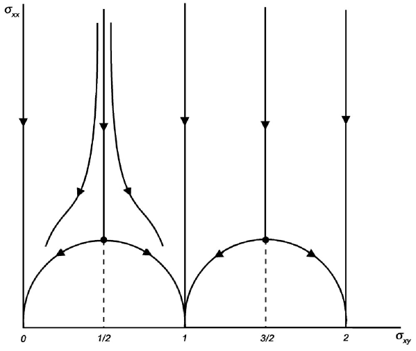
Figure 2: Renormalization group flow diagram for the conductances. The arrows indicate the scaling toward the infrared.

The concept of $\theta$ renormalization originally arose in a series of detailed papers on instantons, based on the background field methodology, that were primarily aimed at a microscopic understanding of the quantum Hall effect [21, 22]. Until to date these pioneering papers have provided most of our insights into the singularity structure of the Grassmannian $U(m+n)/U(m)\times U(n)$ theory at $\theta=\pi$, in particular the case where the number of field components is ‘small’, $0\leqslant m,n\lesssim 1$. Under these circumstances the instanton vacuum at half-integer values of $\sigma_{xy}$ (or $\theta=\pi$) develops a critical fixed point with a finite value of $\sigma_{xx}$ of order unity (see Fig. 2). This indicates that transition at $\theta=\pi$ becomes a true second order quantum phase transition with a non-trivial critical index $\nu$ that changes continuously with varying values of $m$ and $n$ in the range $0\leq m,n\lesssim 1$. This situation is distinctly different from the overwhelming majority of Grassmannian non-linear sigma models with $m,n\gtrsim 1$ for which the scaling diagram is likely to be the same as the one found in the large $N$ expansion (see Fig. 1). In that case one expects a first order phase transition but with a diverging correlation length and a fixed exponent $\nu=1/2$.

The instanton vacuum with $m=n=1$ (the $SU(2)/U(1)$ or O(3) model) is in many ways special. This case is likely to be on the interface between a large $N$-like scaling diagram (see Fig. 1) with a first order transition at $\theta=\pi$, and an instanton driven scaling diagram (see Fig. 2) where the transition is of second order. The expected $m$ and $n$ dependence of quantum criticality is illustrated in Fig. 3 which is the main topic of the present paper (see also Ref. [25]).

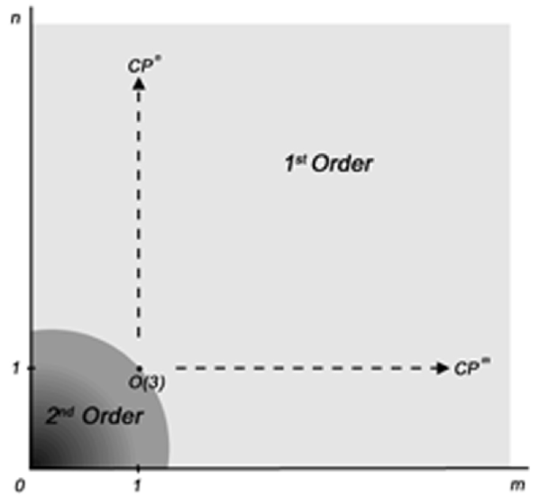
Figure 3: Nature of the transition at $\theta=\pi$ for different values of $m$ and $n$.

1.5 Quantum phase transitions

As is well known, the instanton angle $\theta$ in replica field theory was originally discovered in an attempt to resolve the fundamental difficulties of the scaling theory of Anderson localization in dealing with the quantum Hall effect [3]. However, it was not until the first experiments [6] on the plateau transitions had been conducted that the prediction of quantum criticality in the quantum Hall systems [2] became a well recognized and extensively pursued research objective in physics.

Quantum phase transitions in disordered systems are in many respects quite unusual, from ordinary critical phenomena point of view. For example, such unconventional phenomena like multifractality of the density fluctuations are known to appear as a peculiar aspect of the theory in the replica limit $m=n=0$ [29]. These subtle aspects of disordered systems primarily arose from the non-linear sigma model approach to the Anderson localization problem (mobility edge problem) in $2+\epsilon$ spatial dimensions [30, 31].

The instanton vacuum theory of the quantum Hall effect essentially predicts that the plateau transitions in the two dimensional electron gas behave in all respects like the metal-insulator transition in $2+\epsilon$ dimensions. The reduced dimensionality of the quantum Hall system offers a rare opportunity to perform numerical work on the mobility edge problem and extract accurate results on quantum critical behavior. By now there exists an impressive stock of numerical data on the critical indices of the plateau transitions, including the correlation or localization length exponent ($\nu$) [32, 33, 34, 35, 36, 37], the multifractal $f(\alpha)$ spectrum [38, 39, 40, 41, 42, 43] and even the leading irrelevant exponent ($y_{\sigma}$) in the problem [44, 45].

1.5.1 Quantitative assessments

It is important to know that the laboratory experiments and later the numerical simulations on the plateau transitions in the quantum Hall regime have primarily been guided and motivated by the renormalization group ideas that were originally obtained on the basis of the $\theta$ parameter replica field theory as well as instanton calculus [2, 21, 22]. In addition to this, the more recent discovery of super universality in non-linear sigma models, along with the completely revised insights in the large $N$ expansion, has elucidated the much sought after strong coupling features of the instanton vacuum, notably the quantum Hall effect itself, that previously remained concealed [25]. Both these strong coupling features and the renormalization group results based on instantons have put the theory of an instanton vacuum in a novel physical perspective. Together they provide the complete conceptual framework that is necessary for a detailed understanding of the quantum Hall effect as well as the $\theta$ dependence in the Grassmannian $U(m+n)/U(m)\times U(n)$ non-linear sigma model, for all non-negative values of $m$ and $n$.

In our previous papers we have already presented rough outlines on how the theory manages to interpolate between a large $N$-like scaling diagram for large values of $m,n$ (Fig. 1) and an instanton - driven renormalization behavior for small $m,n$ as indicated in Fig. 2. At present we take the theory several steps further and extend the instanton methodology in several ways. Our main objective is to make detailed predictions on the quantum critical behavior of the theory at $\theta=\pi$ with varying values of $m$ and $n$. We benefit from the fact that this quantum critical behavior is bounded by the theory in the replica limit ($m=n=0$) for which the aforementioned numerical data are available, and the distinctly different $O(3)$ non-linear sigma model ($m=n=1$) for which the critical indices are known exactly. A detailed comparison between our general results and those known for specific examples should therefore provide a stringent and interesting test of the fundamental significance of instantons in the problem.

Our most important results are listed in Table 2 where we compare the critical exponents of the theory with $m=n=0$ with those obtained from numerical simulations on the electron gas. These results clearly demonstrate the validity of a general statement made in Ref. [14, 15, 25] which says that the fundamental significance of the instanton gas is primarily found in the renormalization behavior of the theory or, equivalently, the effective action for chiral edge excitations. This leads to a conceptual understanding of the non-perturbative aspects of the theory that cannot be obtained in any different manner.

1.5.2 Outline of this paper

We start out in Section 2 with an introduction to the formalism, a brief summary of the effective action procedure for massless chiral edge excitations as well as a few comments explaining the super universal features of the instanton vacuum.

The bulk of this work mainly follows the formalism that was introduced in the original papers on instantons [21, 22]. However, the main focus at present is on several important aspects of the theory that previously remained unresolved. The first aspect concerns the ambiguity in the numerical factors that arises in the computation of the instanton determinant. These numerical factors are vitally important since they eventually enter into the renormalization group $\beta$ functions and, hence, determine the critical fixed point properties of the theory. In Section 4 we show how the theory of observable parameters can be used to actually resolve this problem. The final expressions for the $\beta$ functions that we obtain are universal in the sense that they are independent of the specific regularization scheme that is being used.

Secondly, the procedure sofar did not include the effect of mass terms in the theory and, hence, the multifractal aspects of the quantum phase transition have not yet been investigated. The technical difficulties associated with mass terms are quite notorious, however. These have historically resulted in the construction of highly non-trivial extensions of the methodology such as working with constrained instantons [47]. We briefly introduce the subject matter in Section 3 and illustrate the main ideas by means of explicit examples.

It has sofar not been obvious, however, whether the concept of a constrained instanton is any useful in the development a quantum theory. In an earlier paper on the subject  [5] it was pointed out that mass terms in the theory generally involve a different metric tensor than the one that naturally appears in the harmonic oscillator problem, i.e. their geometrical properties are incompatible. These and other complications are avoided in the methodology of spatially varying masses which is based on the various tricks introduced by ’t Hooft in evaluating instanton determinants. In Section 4 we elaborate further on the methodology of Ref. [5] and show that the idea of spatially varying masses generally facilitates explicit computations and yields more relevant results.

In Section 8 we present the detailed predictions of quantum criticality as a function of $m$ and $n$ and make a comparison with the results known from other sources. We end this paper with a conclusion, Section 9.

2 Formalism

2.1 Non-linear sigma model

First we recall the non-linear sigma model defined on the Grassmann manifold $G/H={SU(m+n)}/{S(U(m)\times U(n))}$ and in the presence of the $\theta$ term. We prefer to work in the context of the quantum Hall effect since this provides a clear physical platform for discussing the fundamental aspects of the theory that have previously remained unrecognized. It is easy enough, however, to make contact with the conventions and notations of more familiar models in quantum field theory and statistical mechanics such as the $O(3)$ formalism, obtained by putting $m=n=1$, and the $CP^{N-1}$ model which is obtained by taking $m=N-1$ and $n=1$.

The theory involves matrix field variables $Q(\textbf{r})$ of size $(m+n)\times(m+n)$ that obey the non-linear constraint

$$Q^{2}(\textbf{r})=1_{m+n}.$$ (4)

A convenient representation in terms of ordinary unitary matrices $T(\textbf{r})$ is obtained by writing

$$Q(\textbf{r})=T^{-1}(\textbf{r})\Lambda T(\textbf{r}),\qquad\Lambda=\begin{pmatrix}1_{m}&0\\ 0&-1_{n}\end{pmatrix}.$$ (5)

The action describing the low energy dynamics of the two dimensional electron system subject to a static, perpendicular magnetic field is given by [4]

$$S=-\frac{\sigma_{xx}}{8}\int d\textbf{r}\mathop{\rm tr}\nolimits(\nabla Q)^{2}+\frac{\sigma_{xy}}{8}\int d\textbf{r}\mathop{\rm tr}\nolimits\varepsilon_{ab}Q\nabla_{a}Q\nabla_{b}Q+\omega\rho_{0}\int d\textbf{r}\mathop{\rm tr}\nolimits Q\Lambda.$$ (6)

Here the quantities $\sigma_{xx}$ and $\sigma_{xy}$ represent the meanfield values for the longitudinal and Hall conductances respectively. The $\rho_{0}$ denotes the density of electronic levels in the bulk of the system, $\omega$ is the external frequency and $\varepsilon_{ab}=-\varepsilon_{ba}$ is the antisymmetric tensor.

2.2 Boundary conditions

The second term in Eq. (6) defines the topological invariant $\mathcal{C}[Q]$ which can also be expressed as a one dimensional integral over the edge of the system [21],

$$\mathcal{C}[Q]=\frac{1}{16\pi i}\int d\textbf{r}\mathop{\rm tr}\nolimits\varepsilon_{ab}Q\nabla_{a}Q\nabla_{b}Q=\frac{1}{4\pi i}\oint dx\mathop{\rm tr}\nolimits T\partial_{x}T^{-1}\Lambda.$$ (7)

Here, $\mathcal{C}[Q]$ is integer valued provided the field variable $Q$ equals a constant matrix at the edge. It formally describes the mapping of the Grassmann manifold onto the plane following the homotopy theory result

$$\pi_{2}\left(G/H\right)=\pi_{1}\left(H\right)=\Zset.$$ (8)

To study the $\sigma_{xy}$ dependence of the theory it is in many ways natural to put $\omega=0$ in Eq. (6) and let the infrared of the theory be regulated by the finite system size $L$. The conventional way of defining the $\theta$ vacuum is as follows

$$Z=\int\limits_{\partial V}\mathcal{D}Q\exp\left[-\frac{1}{g}\int d\textbf{r}\mathop{\rm tr}\nolimits(\nabla Q)^{2}+i\theta\,\mathcal{C}[Q]\right],$$ (9)

where the subscript $\partial V$ indicates that the functional integral has to be performed with $Q(\textbf{r})$ kept fixed and constant at the boundary, say $Q=\Lambda$. Under these circumstances the topological charge $\mathcal{C}[Q]$ is strictly integer quantized. The parameter $\theta$ in Eq. (9) is equal to $2\pi\sigma_{xy}$ modulo $2\pi$ and the coupling constant $g$ is identified as $8/\sigma_{xx}$,

$$\theta=2\pi\sigma_{xy}\,{\rm mod}(2\pi),\qquad g=\frac{8}{\sigma_{xx}}.$$ (10)

The theory of Eq. (9), as it stands, is one of the rare examples of an asymptotically free field theory with a vanishing mass gap. What has remarkably emerged over the years is that the theory at $\theta=\pi$ develops a gapless phase that generally can be associated with the transitions between adjacent quantum Hall plateaus. This is unlike the theory with $\theta=0,2\pi$ where the low energy excitations are expected to display a mass gap. The significance of the theory in terms of quantum Hall physics becomes all the more obvious if one recognizes that the mean field parameter $\sigma_{xy}$ for strong magnetic fields is precisely equal to the filling fraction ($\nu$) of the disordered Landau bands

$$\sigma_{xy}=\nu.$$ (11)

This means that the plateau transitions occur at half-integer filling fractions $\nu=k+1/2$ with integer $k$. On the other hand, $\theta=0,2\pi$ corresponds to integer filling fractions $\nu=k$ which generally describe the center of the quantum Hall plateaus.

As was already mentioned in the introduction, the physical objectives of the quantum Hall effect have been - from early onward - in dramatic conflict with the ideas and expectations with which the $\theta$ parameter in quantum field theory was originally perceived. Such fundamental aspects like the existence of robust topological quantum numbers, for example, have previously been unrecognized. This is just one of the reasons why the quantum Hall effect primarily serves as an outstanding laboratory where the controversies in quantum field theory can be explored and investigated in detail.

2.2.1 Massless chiral edge excitations

It has turned out that the theory of Eq. (9) is not yet the complete story. By fixing the boundary conditions in this problem (or by discarding the edge all together) one essentially leaves out fundamental pieces of physics, the massless chiral edge excitations, that eventually will put the strong coupling problem of an instanton vacuum in a novel perspective.

To see how the physics of the edge enters into the problem we consider the case where the Fermi energy of the electron gas is located in an energy gap (Landau gap) between adjacent Landau bands. This is represented by Eq. (6) by putting $\sigma_{xx}=\rho_{0}=0$ and $\sigma_{xy}=k$, i.e. the meanfield value of the Hall conductance is an integer $k$ (in units of $e^{2}/h$) and precisely equal to the number of completely filled Landau bands in the system. Eq. (6) can now be written as follows

$$\hskip 56.9055ptS_{\rm edge}[Q] = 2\pi ik\,\mathcal{C}[Q]+\omega\rho_{\rm edge}\oint dx\mathop{\rm tr}\nolimits Q\Lambda$$ (12)

$$= \oint dx\mathop{\rm tr}\nolimits\left[\frac{k}{2}T\partial_{x}T^{-1}\Lambda+\omega\rho_{\rm edge}Q\Lambda\right].$$

We have added a symmetry breaking term proportional to $\rho_{\rm edge}$ indicating that although the Fermi energy is located in the Landau gap, there still exists a finite density of edge levels ($\rho_{\rm edge}$) that can carry the Hall current. Eq. (12) is exactly solvable and describes long ranged (critical) correlations along the edge of the system. Some important examples of edge correlations are given by [11]

$$\langle Q\rangle_{\rm edge} = \Lambda,$$

$$\hskip 56.9055pt\langle Q_{+-}^{\alpha\beta}(x)Q_{-+}^{\beta\alpha}(x^{\prime})\rangle_{\rm edge} = \vartheta(x^{\prime}-x)\exp\left[-(x^{\prime}-x)\omega\rho_{\rm edge}\right].$$ (13)

Here the expectation is with respect to the one dimensional theory of Eq. (12). The symbol $\vartheta(x)$ stands for the Heaviside step function. These results are the same for all $m$ and $n$, indicating that the massless chiral edge excitations are a generic feature of the instanton vacuum concept.

Eqs (9) and (12) indicate that field configurations with an integral and fractional topological charge ${\mathcal{C}}[Q]$ describe fundamentally different physics and have fundamentally different properties. In the following Sections we show in a step by step fashion how Eq. (12) generally appears as the fixed point action of the strong coupling phase.

2.3 Effective action for the edge

We specialize from now onward to systems with an edge. The main problem next is to see how in general we can separate the bulk pieces of the action from those associated with the edge. The resolution of this problem provides fundamental information on the low energy dynamics of the system (Section 2.3.3) that is intimately related to the Kubo formalism of the conductances (Section 2.3.4). In the end (Sections 2.3.5 and 2.3.6) this leads to the much sought after Thouless’ criterion for the existence of robust topological quantum numbers that explain the precision and observability of the quantum Hall effect.

2.3.1 Bulk and edge field variables

It is convenient to introduce a change of variables

$$Q=t^{-1}Q_{0}t.$$ (14)

Here, $Q_{0}$ is generally defined as a matrix field with $Q_{0}=\Lambda$ at the edge of the system (spherical boundary conditions). The matrix field $t$ describes the fluctuations about these special spherical boundary conditions. It is easy to see that the topological charge $\mathcal{C}[Q]$ can be written as the sum of two separate pieces

$$\mathcal{C}[Q]=\mathcal{C}[t^{-1}Q_{0}t]=\mathcal{C}[Q_{0}]+\mathcal{C}[q],\qquad q=t^{-1}\Lambda t.$$ (15)

Here, the first part $\mathcal{C}[Q_{0}]$ is integer valued whereas the second part $\mathcal{C}[q]$ describes a fractional topological charge,

$$\mathcal{C}[Q_{0}]=k,\qquad-\frac{1}{2}<\mathcal{C}[q]\leq\frac{1}{2}.$$ (16)

It is easy to see that the action for the edge, Eq. (12), only contains the field variable $t$ or $q$ which we shall refer to as the edge fields in the problem. Similarly, the $Q_{0}$ are the only matrix field variables that enter into the usual definition of the $\theta$ vacuum, Eq. (9). We will refer to them as the bulk field variables.

2.3.2 Bulk and edge observables

Next, from Eqs (9) and (12) we infer that the bare or meanfield Hall conductance $\sigma_{xy}$ should in general be split into a bulk piece $\theta(\nu)$ and a distinctly different edge piece $k(\nu)$ as follows (see also Fig. 4)

$$\sigma_{xy}=\nu=\frac{\theta(\nu)}{2\pi}+k(\nu).$$ (17)

Here, $k(\nu)$ is an integer whereas $\theta(\nu)$ is restricted to be in the interval

$$-\pi<\theta(\nu)\leq\pi.$$ (18)

The new symbol $\nu$ indicates that the meanfield parameter $\sigma_{xy}$ is the same as the filling fraction of the Landau bands. Eq. (17) can also be obtained in a more natural fashion and it actually appears as a basic ingredient in the microscopic derivation of the theory.

We use the results to rewrite the topological piece of the action as follows

$$2\pi i\sigma_{xy}\mathcal{C}[Q]=i(\theta(\nu)+2\pi k(\nu))(\mathcal{C}[q]+\mathcal{C}[Q_{0}])=2\pi ik(\nu)\mathcal{C}[q]+i\theta(\nu)\mathcal{C}[Q].$$ (19)

In the second equation we have left out the term that gives rise to unimportant phase factor. Finally we arrive at the following form of the action

$$S=S_{\rm bulk}[t^{-1}Q_{0}t]+S_{\rm edge}[q],$$ (20)

where

$$S_{\rm bulk}[Q]=-\frac{\sigma_{xx}}{8}\int d\textbf{r}\mathop{\rm tr}\nolimits(\nabla Q)^{2}+i{\theta(\nu)}\mathcal{C}[Q]$$ (21)

$$S_{\rm edge}[q]=2\pi ik(\nu)\,\mathcal{C}[q].$$ (22)

Figure 4: The quantity $\sigma_{xy}^{0}=\nu$ is the sum of a quantized edge part $k(\nu)$ and an unquantized bulk part $\theta(\nu)$ .

2.3.3 Response formulae

After these preliminaries we come to the most important part of this Section, namely the definition of the effective action for chiral edge modes $S_{\rm eff}$. This is obtained by formally eliminating the bulk field variable $Q_{0}$ from the theory

$${S_{\rm eff}[q]}=S_{\rm edge}[q]+S^{\,\prime}[q],\qquad\exp S^{\,\prime}[q]=\int\limits_{\partial V}\mathcal{D}[Q_{0}]\exp S_{\rm bulk}[t^{-1}Q_{0}t].$$ (23)

The subscript ${\partial V}$ reminds us of the fact that the functional integral has to be performed with a fixed value $Q_{0}=\Lambda$ at the edge of the system. Next, from symmetry considerations alone it is easily established that $S^{\prime}$ must be of the general form [11]

$$S^{\,\prime}[q]=-\frac{\sigma^{\,\prime}_{xx}}{8}\int\limits d\textbf{r}\mathop{\rm tr}\nolimits(\nabla q)^{2}+i\theta^{\,\prime}\mathcal{C}[q].$$ (24)

We have omitted the higher dimensional terms which generally describe the properties of the electron gas at mesoscopic scales. The most important feature of this result is that the quantities $\sigma^{\prime}_{xx}=\sigma^{\prime}_{xx}(L)$ and $\theta^{\,\prime}=\theta^{\,\prime}(L)$ can be identified with the Kubo formulae for the longitudinal and Hall conductances respectively ($L$ denoting the linear dimension of the system). Notice that these quantities are by definition a measure for the response of the bulk of the system to an infinitesimal change in the boundary conditions (on the matrix field variable $Q_{0}$).

At the same time we can regulate the infrared of the system in a different manner by introducing $U(m)\times U(n)$ invariant mass terms in Eqs (21)-(22)

$$S_{\rm edge}[q]\rightarrow S_{\rm edge}[q]+\omega_{\rm edge}\rho_{\rm edge}\oint dx\mathop{\rm tr}\nolimits\Lambda q,$$ (25)

$$S_{\rm bulk}[t^{-1}Q_{0}t]\rightarrow S_{\rm bulk}[t^{-1}Q_{0}t]+\omega_{0}\rho_{0}\int d\textbf{r}\mathop{\rm tr}\nolimits\Lambda Q_{0}.$$ (26)

The different symbols $\omega_{\rm edge}$ and $\omega_{0}$ indicate that the frequency $\omega$ plays a different role for the bulk fields and edge fields respectively. Notice that the response parameters $\sigma^{\prime}_{xx}$ and $\sigma^{\prime}_{xy}$ in Eq. (24), for $L$ large enough, now depend on frequency $\omega_{0}$ rather than $L$.

$$\sigma^{\prime}_{xx}\rightarrow\sigma^{\prime}_{xx}(\omega_{0}),\qquad\sigma^{\prime}_{xy}\rightarrow\sigma^{\prime}_{xy}(\omega_{0})=k(\nu)+\frac{\theta^{\,\prime}(\omega_{0})}{2\pi}.$$ (27)

2.3.4 Background field methodology

Let us next go back to the background field methodology and notice the subtle differences with the effective action procedure as considered here. In this methodology we consider a slowly varying but fixed background matrix field $b$ that is applied directly to the original theory of Eq. (6),

$$\exp S_{\rm eff}[b^{-1}\Lambda b] = \int\mathcal{D}Q\exp\left(S_{\sigma}[b^{-1}Qb]+\omega_{0}\rho_{0}\int d\textbf{r}\mathop{\rm tr}\nolimits Q\Lambda\right),$$ (28)

$$S_{\sigma}[Q] = -\frac{\sigma_{xx}}{8}\int d\textbf{r}\mathop{\rm tr}\nolimits(\nabla Q)^{2}+2\pi i\sigma_{xy}\,\mathcal{C}[Q].$$

Here, $S_{\rm eff}$ can again be written in the following general form

$$S_{\rm eff}[q_{b}]=-\frac{\sigma^{\prime}_{xx}(\omega_{0})}{8}\int d\textbf{r}\mathop{\rm tr}\nolimits(\nabla q_{b})^{2}+2\pi i\sigma^{\prime}_{xy}(\omega_{0})\mathcal{C}[q_{b}],$$ (29)

where now $q_{b}=b^{-1}\Lambda b$. Notice that an obvious difference with the situation before is that the functional integral in Eq. (28) is now performed for an arbitrary matrix field $Q$ whereas in Eq. (23) the $Q_{0}$ is always restricted to have $Q_{0}=\Lambda$ at the edge. However, as long as one works with a finite frequency $\omega_{0}$ the boundary conditions on the $Q_{0}$ field are immaterial and the response parameters in Eq. (27) and those in Eq. (29) should be identically the same. As an important check on these statements we consider $\sigma_{xx}=0$ and $\sigma_{xy}=k$, i.e. $S_{\sigma}$ equals the action for the edge $S_{\textrm{edge}}$. In this case Eq. (29) is obtained as follows

$$\exp S_{\rm eff}[q_{b}] = \int{\mathcal{D}}Q\exp\left[\oint dx\left(\frac{k}{2}\mathop{\rm tr}\nolimits Tb\partial_{x}b^{-1}T^{-1}\Lambda+\omega\rho_{edge}\mathop{\rm tr}\nolimits Q\Lambda\right)\right]$$ (30)

$$= \left(\int{\mathcal{D}}Q\exp{S_{\textrm{edge}}[Q]}\right)\,\exp\left[\frac{k}{2}\oint dx\mathop{\rm tr}\nolimits b\partial_{x}b^{-1}\langle Q\rangle_{\textrm{edge}}\right].$$

Using Eq. (13) we can write, discarding constants,

$${S_{\rm eff}[q_{b}]}=2\pi ik~{}{\mathcal{C}}[q_{b}]$$ (31)

Comparing Eqs (29) and (31) we see that $\sigma_{xx}^{\prime}=0$ and $\sigma_{xy}^{\prime}=k$ as it should be. Notice that we obtain essentially the same result if instead of integrating we fix the $Q=\Lambda$ at the edge.

Eq. (30) clearly demonstrates why critical edge correlations should be regarded as a fundamental aspect of the instanton vacuum concept. If, for example, $S_{\textrm{edge}}$ were to display gapped excitations at the edge then we certainly would have $\langle Q\rangle_{\textrm{edge}}=0$ in Eq. (30) and instead of Eq. (31) we would have had a vanishing Hall conductance!

This, then, would be serious conflict with the quantum Hall effect which says that the quantization of the Hall conductance is in fact a robust phenomenon.

2.3.5 Thouless criterion

We next show that a Thouless criterion [23] for the quantum Hall effect can be obtained directly, as a corollary of the aforementioned effective action procedure. For this purpose we notice that if the system develops a mass gap or a finite correlation length $\xi$ in the bulk, then the theory of $S_{\textrm{bulk}}$, Eq. (21), should be insensitive to any changes in the boundary conditions, provided the system size $L$ is large enough. Under these circumstances the response quantities $\sigma^{\prime}_{xx}(L)$ and $\theta^{\,\prime}(L)$ in Eq. (24) should vanish. In terms of the conductances we can write

$$\sigma^{\prime}_{xx}(L)=\mathcal{O}\left(e^{-L/\xi}\right),\qquad\sigma^{\prime}_{xy}(L)=k(\nu)+\frac{\theta^{\prime}(L)}{2\pi}=k(\nu)+\mathcal{O}\left(e^{-L/\xi}\right).$$ (32)

This important result indicates that the quantum Hall effect is in fact a universal, strong coupling feature of the $\theta$ vacuum, independent of the number of field components $m$ and $n$. The fixed point action of the quantum Hall state is generally given by the one dimensional action [11]

$$S_{\rm eff}[q]=\oint dx\mathop{\rm tr}\nolimits\left[\frac{k(\nu)}{2}t\partial_{x}t^{-1}\Lambda+\omega\rho_{\rm edge}q\Lambda\right],$$ (33)

which is none other than the aforementioned action for massless chiral edge excitations.

In summary we can say that the background field methodology that was previously introduced for renormalization group purposes alone, now gets a new appearance in the theory and a fundamentally different meaning in term of the effective action for massless edge excitations. This effective action procedure emerges from the theory itself and, unlike the background field methodology, it provides the much sought after Thouless criterion which associates the exact quantization of the Hall conductance with the insensitivity of the bulk of the system to changes in the boundary conditions.

2.3.6 Conductance fluctuations, level crossing

The definition of the effective action, Eq. (23), implies that the exact expression for $S_{\rm eff}$ is invariant under a change in the matrix field $t\rightarrow Ut$, i.e. the replacement

$$S_{\rm eff}[t^{-1}\Lambda t]\rightarrow S_{\rm eff}[t^{-1}U^{-1}\Lambda Ut]$$ (34)

should leave the theory invariant. Here, the $U=U(\textbf{r})$ represents a unitary matrix field with an integer valued topological charge, i.e. $U(\textbf{r})$ reduces to an arbitrary $U(m)\times U(n)$ gauge at the edge of the system.

Notice that the expressions for $S_{\rm eff}$, Eqs (23) and (24), in general violate the invariance under Eq. (34). This is so because we have expressed $S^{\,\prime}[q]$ to lowest order in a series expansion in powers of the derivatives acting on the $q$ field. If the response parameters $\sigma^{\prime}_{xx}(L)$ and $\theta^{\prime}(L)$ are finite then the invariance under Eq. (34) is generally broken at each and every order in the derivative expansion. The invariance is truly recovered only after the complete series is taken into account, to infinite order. This situation typically describes a gapless phase in the theory. The infinite series (or at least an infinite subset of it) can in general be rearranged and expressed in terms of probability distributions for the response parameters $\sigma^{\prime}_{xx}(L)$ and $\theta^{\prime}(L)$. Quantum critical points, for example, seem to generically display broadly distributed response parameters. The large $N$ expansion has provided, once more, a lucid and exact example of these statements [25].

On the other hand, if the theory displays a mass gap then each term in the series for $S^{\prime}[q]$ should vanish, i.e. the response parameters are all exponentially small in the system size. It is therefore possible to employ Eq. (34) as an alternative criterion for the quantum Hall effect, namely by demanding that the theory be invariant under Eq. (34) order by order in the derivative expansion. This criterion immediately demands that $\sigma^{\prime}_{xx}$ and $\theta^{\prime}$ in Eq. (24) be zero and the effective action be given by Eq. (33). Equations (33) and (34) imply

$$S_{\rm eff}[t^{-1}U^{-1}\Lambda Ut]=S_{\rm eff}[t^{-1}\Lambda t]+2\pi ik(\nu){\mathcal{C}}[U^{-1}\Lambda U].$$ (35)

Although the matrix $U$ merely gives rise to a phase factor that can be dropped, physically it corresponds to an integer number $n_{e}$ of (edge) electrons, equal to $k(\nu){\mathcal{C}}[U^{-1}\Lambda U]$, that have crossed the Fermi level. Eq. (35) is therefore synonymous for the statement which says that the quantization of the Hall conductance $\sigma_{xy}=k(\nu)\left[e^{2}/h\right]$ is related to the quantization of flux $\Phi={\mathcal{C}}[U^{-1}\Lambda U]\left[h/e\right]$ and quantization of charge $q_{e}=n_{e}\left[e\right]$ according to

$$q_{e}=\sigma_{xy}\Phi.$$ (36)

2.4 Physical observables

The response parameters $\sigma^{\prime}_{xx}$ and $\theta^{\prime}$ as well as other observables, associated with the mass terms in the non-linear sigma model, are in many ways the most significant physical quantities in the theory that contain complete information on the low energy dynamics of the instanton vacuum. These quantities can all be expressed in terms of correlation functions of the bulk field variables $Q_{0}$ alone. In this Section we give a summary of the physical observables in the theory which then completes the theory of massless chiral edge excitations.

To start we introduce the following theory for the bulk matrix field variables (dropping the subscript “$0$” on the $Q_{0}$ from now onward)

$$Z=\int\limits_{\partial V}\mathcal{D}Q\exp\left(S_{\sigma}[Q]+S_{h}[Q]+S_{a}[Q]+S_{s}[Q]\right).$$ (37)

The subscript $\partial V$ indicates, as before, that the $Q$ is kept fixed at $Q=\Lambda$ at the edge of the system. $S_{\sigma}$ stands for

$$S_{\sigma}[Q]=-\frac{\sigma_{xx}}{8}\int d\textbf{r}\mathop{\rm tr}\nolimits(\nabla Q)^{2}+\frac{\theta}{16\pi}\int d\textbf{r}\mathop{\rm tr}\nolimits\varepsilon_{ab}Q\nabla_{a}Q\nabla_{b}Q.$$ (38)

The quantities $S_{h}$, $S_{a}$ and $S_{s}$ are the $U(m)\times U(n)$ invariant mass terms that will be specified below.

2.4.1 Kubo formula

Explicit expressions for response quantities $\sigma^{\prime}_{xx}$ and $\theta^{\prime}$ can be derived following the analysis of Ref. [22]. The following $U(m)\times U(n)$ invariant results have been obtained

$$\sigma_{xx}^{\prime}=\sigma_{xx} + \frac{\sigma_{xx}^{2}}{16mnL^{2}}\int d\textbf{r}d\textbf{r}^{\prime}\mathop{\rm tr}\nolimits\langle Q(\textbf{r})\nabla Q(\textbf{r})Q(\textbf{r}^{\prime})\nabla Q(\textbf{r}^{\prime})\rangle,$$ (39)

$$\theta^{\prime}=\theta - \frac{(m+n)\pi}{4mnL^{2}}\sigma_{xx}\int d\textbf{r}\mathop{\rm tr}\nolimits\langle\Lambda Q\varepsilon_{ab}r_{a}\partial_{b}Q\rangle$$ (40)

$$+ \frac{\pi\sigma_{xx}^{2}}{8mnL^{2}}\int d\textbf{r}d\textbf{r}^{\prime}\mathop{\rm tr}\nolimits\varepsilon_{ab}\langle Q(\textbf{r})\nabla_{a}Q(\textbf{r})Q(\textbf{r}^{\prime})\nabla_{b}Q(\textbf{r}^{\prime})\Lambda\rangle.$$

Here and from now onward the expectations are defined with respect to the theory of Eq. (37).

2.4.2 Mass terms

We shall be interested in traceless $U(m)\times U(n)$ invariant operators that are linear in $Q$ $(O_{h})$ and bilinear in $Q$ $(O_{s,a})$,

$$S_{h}[Q]=z_{h}\int d\textbf{r}\,O_{h}[Q],\qquad S_{a,s}[Q]=z_{a,s}\int d\textbf{r}\,O_{a,s}[Q].$$ (41)

Here,

$$O_{h}[Q]=\mathop{\rm tr}\nolimits\left[\Lambda-\frac{m-n}{m+n}1_{m+n}\right]Q.$$ (42)

The bilinear operators generally involve a symmetric and an antisymmetric combination [31]

$$O_{s,a}[Q]=\sum\limits_{p,q}^{\alpha,\beta}K_{s,a}^{pq}\left[Q_{pp}^{\alpha\alpha}Q_{qq}^{\beta\beta}\pm Q_{pq}^{\alpha\beta}Q_{qp}^{\beta\alpha}\right],$$ (43)

where $K_{s,a}$ is given as a $2\times 2$ matrix

$$K_{s,a}=\begin{pmatrix}-\displaystyle\frac{m}{n\pm 1}&1\\ 1&-\displaystyle\frac{n}{m\pm 1}\end{pmatrix}.$$ (44)

These quantities permit us to define physical observables $z_{h}^{\prime}$ and $z^{\prime}_{s,a}$ that are associated with the $z_{h}$ and $z_{s,a}$ fields respectively. Specifically,

$$z_{h}^{\prime}=z_{h}\frac{\langle O_{h}[Q]\rangle}{O_{h}[\Lambda]},\quad z^{\prime}_{s}=z_{s}\frac{\langle O_{s}[Q]\rangle}{O_{s}[\Lambda]},\quad z^{\prime}_{a}=z_{a}\frac{\langle O_{a}[Q]\rangle}{O_{a}[\Lambda]}.$$ (45)

The ratio on the right hand side merely indicates that the expectation value of the operators is normalized with respect to the classical value.

2.4.3 $\beta$ and $\gamma$ functions

The observable parameters of the previous Sections facilitate a renormalization group study that can be extended to include the non-perturbative effects of instantons. Since much of the analysis is based on the theory in $2+\epsilon$ spatial dimensions [31] we shall first recapitulate some of the results obtained from ordinary perturbative expansions. Let $\mu^{\prime}$ denote the momentum scale associated with the observable theory then the quantities $\sigma^{\prime}_{xx}=\sigma_{xx}(\mu^{\prime})$, $z_{i}^{\prime}=z_{i}(\mu^{\prime})$ can be expressed in terms of the renormalization group $\beta$ and $\gamma$ functions according to (see Appendix  A)

$$\hskip 71.13188pt\sigma^{\prime}_{xx} = \sigma_{xx}(\mu^{\prime})=\sigma_{xx}(\mu_{0})+\int_{\mu_{0}}^{\mu^{\prime}}\frac{d\mu}{\mu}~{}\beta_{\sigma}(\sigma_{xx})$$ (46)

$$z_{i}^{\prime} = z_{i}(\mu^{\prime})=z_{i}(\mu_{0})-\int_{\mu_{0}}^{\mu^{\prime}}\frac{d\mu}{\mu}~{}\gamma_{i}(\sigma_{xx})z_{i}(\mu),$$ (47)

where [48]

$$\hskip 85.35826pt\beta_{\sigma}(\sigma_{xx}) = \frac{m+n}{2\pi}+\frac{mn+1}{2\pi^{2}\sigma_{xx}}+{\mathcal{O}}(\sigma_{xx}^{-2})$$ (48)

$$\gamma_{h}(\sigma_{xx}) = -\frac{m+n}{2\pi\sigma_{xx}}+{\mathcal{O}}(\sigma_{xx}^{-2})$$ (49)

$$\gamma_{s}(\sigma_{xx}) = -\frac{m+n+2}{2\pi\sigma_{xx}}+{\mathcal{O}}(\sigma_{xx}^{-2})$$ (50)

$$\gamma_{a}(\sigma_{xx}) = -\frac{m+n-2}{2\pi\sigma_{xx}}+{\mathcal{O}}(\sigma_{xx}^{-2}).$$ (51)

The effects of instantons have been studied in great detail in Refs [3, 4] where the idea of the $\theta$ renormalization was introduced. The main objective of the present paper is to extend the results of Eqs (46)-(51) to include the effect of instantons. Recall that the $\gamma_{i}$ functions are of very special physical interest. For example, the quantity $\gamma_{h}$ should vanish in the limit $m,n\rightarrow 0$ indicating that the density of levels of the electron gas is in general unrenormalized. At the same time one expects the anomalous dimension $\gamma_{a}$ to become positive as $m,n\rightarrow 0$ since it physically describes the singular behavior of the (inverse) participation ratio of the electronic levels. These statements serve as an important physical constraint that one in general should impose upon the theory [31].

3 Instantons

3.1 Introduction

In the absence of symmetry breaking terms, the existence of finite action solutions (instantons) follows from the Schwartz inequality

$$\mathop{\rm tr}\nolimits\left[\nabla_{x}Q\pm iQ\nabla_{y}Q\right]^{2}\geq 0,$$ (52)

which implies

$$\frac{1}{8}\int d\textbf{r}\mathop{\rm tr}\nolimits(\nabla Q)^{2}\geq 2\pi|\mathcal{C}[Q]|.$$ (53)

Matrix field configurations that fulfill inequality (53) as an equality are called instantons. The classical action becomes

$$S_{\sigma}^{\rm inst}=-2\pi\sigma_{xx}|\mathcal{C}[Q]|+\,i\theta\mathcal{C}[Q].$$ (54)

In this paper we consider single instantons only with a topological charge $\mathcal{C}[Q]=\pm 1$. A convenient representation of the single instanton solution is given by  [21, 22]

$$Q_{\rm inst}(\textbf{r})=T^{-1}{\Lambda}_{\rm inst}(\textbf{r})T,\qquad\Lambda_{\rm inst}(\textbf{r})=\Lambda+\rho(\textbf{r}).$$ (55)

Here, the matrix $\rho^{\alpha\beta}_{pq}(\textbf{r})$ has four non-zero matrix elements only

$$\rho^{11}_{11}=-\rho^{11}_{-1-1}=-\frac{2\lambda^{2}}{|z-z_{0}|^{2}+\lambda^{2}},\qquad\rho^{11}_{1-1}=\bar{\rho}^{11}_{-11}=\frac{2\lambda(z-z_{0})}{|z-z_{0}|^{2}+\lambda^{2}},$$ (56)

with $z=x+iy$. The quantity $z_{0}$ describes the position of the instanton and $\lambda$ is the scale size. These parameters, along with the global unitary rotation $T\in U(m+n)$, describe the manifold of the single instanton. The anti-instanton solution with topological charge $\mathcal{C}[Q]=-1$ is simply obtained by complex conjugation.

Next, to discuss the mass terms in the theory, we substitute Eq. (55) into Eqs (42) and (43). Putting $T=1_{m+n}$ for the moment then one can split the result for the operators $O_{i}$ into a topologically trivial part and an instanton part as follows

$$O_{i}[Q_{\rm inst}]=O_{i}[\Lambda_{\rm inst}]=O_{i}[\Lambda]+O_{i}^{\rm inst}(\textbf{r}),$$ (57)

where

$$O_{h}[\Lambda]=\frac{4mn}{m+n},\quad O_{a}[\Lambda]=-4mn,\quad O_{s}[\Lambda]=-4mn$$ (58)

and

$$O_{h}^{\rm inst}(\textbf{r})=2\rho_{11}^{11}(\textbf{r}),\qquad O_{a}^{\rm inst}(\textbf{r})=-{4(m+n-1)}\rho_{11}^{11}(\textbf{r})$$

$$O_{s}^{\rm inst}(\textbf{r})=-{4(m+n+1)}\rho_{11}^{11}(\textbf{r})\left(1+\frac{2\rho_{11}^{11}(\textbf{r})}{m+n+2}\right).$$ (59)

Similarly we can write the free energy as the sum of two parts

$$\mathcal{F}^{class}=\mathcal{F}_{0}^{class}+\mathcal{F}_{\rm inst}^{class},$$ (60)

where $\mathcal{F}_{0}^{class}$ denotes the contribution of the trivial vacuum with topological charge equal to zero ($Q=\Lambda$) and $\mathcal{F}_{\rm inst}^{class}$ is the instanton part

$$\mathcal{F}_{0}^{class}=z_{h}\int d\textbf{r}O_{h}[\Lambda]+z_{s}\int d\textbf{r}O_{s}[\Lambda]+z_{a}\int d\textbf{r}O_{a}[\Lambda]$$ (61)

$$\hskip 42.67912pt\mathcal{F}_{\rm inst}^{class}=\int\limits_{\rm inst}\exp\Bigl{[} - 2\pi\sigma_{xx}\pm\,i\theta+z_{h}\int d\textbf{r}O_{h}^{\rm inst}(\textbf{r})$$ (62)

$$+ z_{s}\int d\textbf{r}O_{s}^{\rm inst}(\textbf{r})+z_{a}\int d\textbf{r}O_{a}^{\rm inst}(\textbf{r})\Bigr{]}.$$

The subscript “$\rm inst$” on the integral sign indicates that the integral is in general to be performed over the manifold of instanton parameters. Notice, however, that the global matrix $T$ is no longer a part of the instanton manifold except for the subgroup $U(m)\times U(n)$ only that leaves the action invariant. In the presence of the mass terms we therefore have, instead of Eq. (55),

$$Q_{\rm inst}(\textbf{r})=W^{-1}{\Lambda}_{\rm inst}(\textbf{r})W=\Lambda+W^{-1}\rho(\textbf{r})W$$ (63)

with $W\in U(m)\times U(n)$. On the other hand, the spatial integrals in the exponential of Eq. (62) still display a logarithmic divergence in the size of the system. To deal with these and other complications we shall in this paper follow the methodology as outlined in Ref. [5]. Before embarking on the quantum theory, however, we shall first address the idea of working with constrained instantons.

3.2 Constrained instantons

It is well known that the discrete topological sectors do not in general have stable classical minima for finite values of $z_{i}=0$. It is nevertheless possible construct matrix field configurations that minimize the action under certain fixed constraints. In this Section we are interested in finite action field configurations $Q$ that smoothly turn into the instanton solution of Eq. (63) in the limit where the symmetry breaking fields $z_{i}$ all go to zero. Although the methodology of this paper avoids the idea of constrained instantons all together, the problem nevertheless arises in the discussion of a special aspect of the theory, the replica limit (Section 7.5). To simplify the analysis we will consider the theory in the presence of the $S_{h}$ term only.

3.2.1 Explicit solution

To obtain finite action configurations for finite values of $z_{h}$ it is in many ways natural to start from the original solution of Eq. (63) and minimize the action with respect to a spatially varying scale size $\lambda(\textbf{r})$ rather than a spatially independent parameter $\lambda$. Write

$$\lambda^{2}\rightarrow\lambda^{2}(\textbf{r})=\lambda^{2}f\left(x,\tilde{h}^{2}\right),$$ (64)

where $f(x,\tilde{h}^{2})$ is a dimensionless function of the dimensionless quantities $x={r^{2}}/{\lambda^{2}}$ and $\tilde{h}^{2}=4z_{h}\lambda^{2}/\sigma_{xx}$ respectively. The strategy is to find an optimal function $f$ with the following constraints

$$\hskip 142.26378ptf(x,0) = 1$$ (65)

$$f(0,\tilde{h}^{2}) = 1$$ (66)

$$f(x\rightarrow\infty,\tilde{h}^{2}>0) = 0.$$ (67)

The first of these equations ensures that in the absence of mass terms ($z_{h}=\tilde{h}^{2}=0$) we regain the original instanton solution. The second and third ensure that the classical action is finite for finite values of $z_{h}$ or $\tilde{h}^{2}$.

It is easy to see that for all functions $f(x,\tilde{h}^{2})$ satisfying Eqs (65) - (67) the topological charge equals unity, i.e.

$$\mathcal{C}[Q]=\int\limits_{0}^{\infty}dx\frac{f-x\partial_{x}f}{(x+f)^{2}}=1.$$ (68)

Next, the expression for the action becomes (discarding the constant terms in the definition of $S_{h}$)

$$S_{\sigma}+S_{h}=-\pi\sigma_{xx}\int\limits_{0}^{\infty}dx\Bigl{\{}\frac{f}{(x+f)^{2}}\Bigl{[}1+\Bigl{(}1-\frac{x\partial_{x}f}{f}\Bigr{)}^{2}\Bigr{]}+\tilde{h}^{2}\frac{f}{x+f}\Bigr{\}}.$$ (69)

The function $f_{0}(x,\tilde{h}^{2})$ that optimizes the action satisfies the following equation

$$-x[2\partial^{2}_{x}f_{0}-f_{0}(\partial_{x}f_{0})^{2}]+2\frac{f_{0}\partial_{x}f_{0}}{x+f_{0}}[x\partial_{x}f_{0}-2f_{0}]+\tilde{h}^{2}f^{2}_{0}=0.$$ (70)

We are generally interested in the limit $\tilde{h}^{2}\ll 1$ only. Eq. (70) cannot be solved analytically. The asymptotic behavior of $f_{0}(x,\tilde{h}^{2})$ in the limit of large and small values of $x$ is obtained as follows. For $x\gg 1$, we find

$$f_{0}(x,\tilde{h}^{2})\propto\tilde{h}^{2}xK^{2}_{1}(\tilde{h}\sqrt{x})=\begin{cases}\displaystyle\frac{\pi\tilde{h}}{2}\sqrt{x}\exp(-2\tilde{h}\sqrt{x}),&\quad x\gg\tilde{h}^{-2},\\ \displaystyle 1+\tilde{h}^{2}x\ln\frac{\tilde{h}\sqrt{x}}{2},&\quad\tilde{h}^{-2}\gg x\gg 1.\end{cases}$$ (71)

Here, $K_{1}(z)$ stands for the modified Bessel function. In the regime $x\ll 1$ we obtain

$$f_{0}(x,\tilde{h}^{2})\approx 1+4\tilde{h}^{2}x,\qquad x\ll 1.$$ (72)

Notice that these asymptotic results can also be written more simply as follows

$$f_{0}(x,\tilde{h}^{2})\approx\begin{cases}\displaystyle\frac{\pi}{2}hr\exp(-2hr),&\quad r\gg h^{-1}\\ \displaystyle 1+(hr)^{2}\ln\frac{hr}{2},&\quad h^{-1}\gg r\gg\lambda\\ 1+4(hr)^{2},&r\ll\lambda.\end{cases}$$ (73)

In the intermediate regimes $r\approx\lambda$ and $r\approx h^{-1}$ we have obtained the solution numerically. In Fig. 5 we plot the results in terms of the matrix element $\rho^{11}_{11}(r)$, Eq. (56),

$$\rho^{11}_{11}(r)=-\frac{2\lambda}{r^{2}+\lambda^{2}}\rightarrow-\frac{2f}{x+f}.$$ (74)

Comparing the result with $\tilde{h}^{2}=0.3$ with the original instanton result, $f=1$, we see that the main difference is in the asymptotic behavior with large $r$ where the $\rho^{11}_{11}$ for the “constrained instanton” vanishes exponentially ($\propto\exp(-2hr)$), rather than algebraically ($\propto 1/r^{2}$).

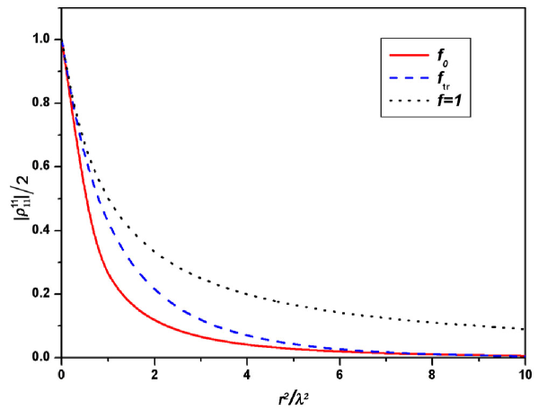
Figure 5: The matrix element $|\rho_{11}^{11}|/2$ as the function of $r^{2}/\lambda^{2}$ for $\tilde{h}^{2}=0.3$.

3.2.2 Finite action

We conclude that in the presence of the mass term $S_{h}$ the requirement of finite action forces the instanton scale size to become spatially dependent in general such that the contributions from large distances $r\gg h^{-1}$ are strongly suppressed in the spatial integrals. On the other hand, from Eqs (71) and (72) one can also see that for small scale sizes $\lambda$ such that

$$\lambda\ll\lambda_{h}\propto h^{-1},$$ (75)

the dominant contribution comes from the original, unconstrained instanton solution of Eq. (55).

In order to see the effect of the constrained instanton on the analytic form of the action we first consider a simpler example of a trial function $f_{\rm tr}(x)$ of the type

$$f_{\rm tr}(x)=\exp(-ax).$$ (76)

Here we use $a$ as a variational parameter. The classical action becomes

$$S_{\sigma}+S_{h}=-2\pi\sigma_{xx}\Bigl{[}1+\frac{a}{2}+\frac{\tilde{h}^{2}}{2}\Bigl{(}\ln\frac{1}{a}-\gamma\Bigr{)}\Bigr{]}+\mathcal{O}(\tilde{h}^{4}),$$ (77)

where the constant $\gamma\approx 0.577$ stands for the Euler constant. The optimal value of $a$ is given by

$$a=\tilde{h}^{2},\qquad f_{\rm tr}(x)=\exp(-\tilde{h}^{2}x).$$ (78)

Hence we find for Eq. (77)

$$S_{\sigma}+S_{h}=-2\pi\sigma_{xx}\Bigl{[}1+\frac{\tilde{h}^{2}}{2}\ln\frac{1.53}{\tilde{h}^{2}}\Bigr{]}.$$ (79)

This simple result obtained from the trial function (78) has the same asymptotic form as one determined by the much more complicated optimal function $f_{0}(x)$ in the limit $\tilde{h}^{2}\rightarrow 0$, except that the numerical constant $1.53$ is replaced by $0.85$.

Eq. (79) indicates that that in the limit $h\rightarrow 0$ the finite action of the constrained instanton smoothly goes over into the finite action of the unconstrained instanton. Furthermore, it is easy to see that the final result of Eq. (79) has precisely the features that one would normally associate with mass terms. Consider for example the action of the unconstrained instanton with a fixed scale size $\lambda$. By putting the system inside a large circle of radius $R$ we obtain the following result

$$S_{\sigma}+S_{h}=-2\pi\sigma_{xx}\Bigl{[}1-\frac{\lambda^{2}}{R^{2}}+\frac{\tilde{h}^{2}}{2}\ln\frac{R^{2}}{\lambda^{2}}\Bigr{]}.$$ (80)

By comparing Eq. (79) and Eq. (80) we conclude that the following effective size $R_{h}$ is induced by the $h$ field

$$R_{h}=\frac{1.47}{h}.$$ (81)

The effect of mass terms can therefore be summarized as follows. First, the integral over scale sizes $\lambda$ (see Eq. (62)) effectively proceeds over the interval $\lambda\lesssim h^{-1}$. Secondly, the spatial integrals in the theory are cut off in infrared and the effective sample size equals $R_{h}$. The two different scales that are being induced by $S_{h}$, $h^{-1}$ and $R_{h}$, are of the same order of magnitude.

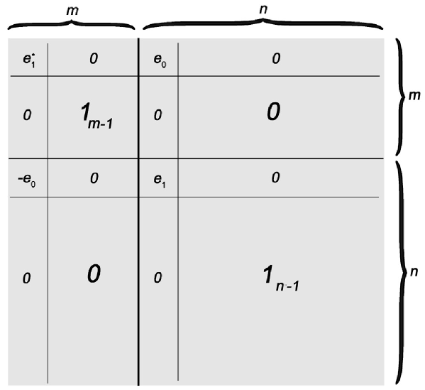
Figure 6: The matrix $R$.

4 Quantum theory

One of the problems with the idea of constrained instantons is that it does not facilitate an expansion of the theory about $z_{i}=0$ in any obvious fashion. This is unlike the method of spatially varying masses which is based on the results obtained in Ref. [21] and [22]. To start we first recapitulate the formalism of the theory without mass terms in Section 4.1. In Section 4.2 we introduce the idea of spatially varying masses. Finally, in Section 4.3 we present the complete action of the small oscillator problem that will be used in the remainder of this paper.

4.1 Preliminaries

To obtain the most general matrix field variable $Q$ with topological charge equal to unity we first rewrite the instanton solution $\Lambda_{\rm inst}$ in Eqs (55) and (56) as a unitary rotation $R$ about the trivial vacuum $\Lambda$

$$\Lambda_{\rm inst}=R^{-1}\Lambda R$$ (82)

where

$$R=\begin{pmatrix}\delta^{\alpha\beta}+(\bar{e}_{1}-1)\delta^{\alpha 1}\delta^{\beta 1}&e_{0}\delta^{\alpha 1}\delta^{\beta 1}\\ -e_{0}\delta^{\alpha 1}\delta^{\beta 1}&\delta^{\alpha\beta}+(e_{1}-1)\delta^{\alpha 1}\delta^{\beta 1}\end{pmatrix}.$$ (83)

The quantities $e_{0}$ and $e_{1}$ are defined as

$$e_{0}=\frac{\lambda}{\sqrt{|z-z_{0}|^{2}+\lambda^{2}}},\qquad e_{1}=\frac{z-z_{0}}{\sqrt{|z-z_{0}|^{2}+\lambda^{2}}}.$$ (84)

For illustration we have written the full matrix $R^{\alpha\beta}_{pp^{\prime}}$ in Fig. 6. It is a simple matter to next generalize these expressions and the result is

$$Q=T^{-1}_{0}R^{-1}q\,R\,T_{0}.$$ (85)

Here, $T_{0}$ denotes a global $U(m+n)$ rotation. The matrix $q$ with $q^{2}=1_{m+n}$ represents the small fluctuations about the one instanton. Write

$$q=w+\Lambda\sqrt{1_{m+n}-w^{2}}$$ (86)

with

$$w=\begin{pmatrix}0&v\\ v^{\dagger}&0\end{pmatrix}$$ (87)

then the matrix $q$ can formally be written as a series expansion in powers of the $m\times n$ complex matrices $v$, $v^{{\dagger}}$ which are taken as the independent field variables in the problem.

4.1.1 Stereographic projection

Eq. (85) lends itself to an exact analysis of the small oscillator problem. First we recall the results obtained for the theory without mass terms [21, 22],

$$\frac{\sigma_{xx}}{8}\int d\textbf{r}\mathop{\rm tr}\nolimits(\nabla Q)^{2}=\frac{\sigma_{xx}}{8}\int d\textbf{r}\mathop{\rm tr}\nolimits[\nabla+\textbf{A},q]^{2},$$ (88)

where the matrix A contains the instanton degrees of freedom

$$\textbf{A}=RT_{0}\nabla T^{-1}_{0}R^{-1}=R\nabla R^{-1}.$$ (89)

By expanding the $q$ in Eq. (88) to quadratic order in the quantum fluctuations $v$, $v^{\dagger}$ we obtain the following results

$$\frac{\sigma_{xx}}{8}\int d\textbf{r}\mathop{\rm tr}\nolimits[\nabla+\textbf{A},q]^{2}=\frac{\sigma_{xx}}{4}\int d\textbf{r}\mu^{2}(\textbf{r})\Biggl{[}v^{11}O^{(2)}v^{{\dagger}11}+\sum\limits_{\alpha=2}^{m}v^{\alpha 1}O^{(1)}v^{{\dagger}1\alpha}$$

$$+\sum\limits_{\beta=2}^{n}v^{1\beta}O^{(1)}v^{{\dagger}\beta 1}+\sum\limits_{\alpha=2}^{m}\sum\limits_{\beta=2}^{n}v^{\alpha\beta}O^{(0)}v^{{\dagger}\beta\alpha}\Biggr{]}.$$ (90)

The three different operators $O^{(a)}$ are given as

$$O^{(a)}=\frac{(r^{2}+\lambda^{2})^{2}}{4\lambda^{2}}\left[\nabla_{b}+\frac{ia\varepsilon_{bc}r_{c}}{r^{2}+\lambda^{2}}\right]^{2}+\frac{a}{2}.$$ (91)

The introduction of a measure $\mu^{2}(\textbf{r})$ for the spatial integration in Eq. (90),

$$\mu(\textbf{r})=\frac{2\lambda}{r^{2}+\lambda^{2}},$$ (92)

indicates that the quantum fluctuation problem is naturally defined on a sphere with radius $\lambda$. It is convenient to employ the stereographic projection

$$\eta=\frac{r^{2}-\lambda^{2}}{r^{2}+\lambda^{2}},\qquad-1<\eta<1$$ (93)

$$\theta=\tan^{-1}\frac{y}{x},\qquad 0\leq\theta<2\pi.$$ (94)

In terms of $\eta$, $\theta$ the integration can be written as

$$\int d\textbf{r}\mu^{2}(\textbf{r})=\int d\eta d\theta.$$ (95)

Moreover,

$$e_{0}=\sqrt{\frac{1-\eta}{2}},\qquad\qquad e_{1}=\sqrt{\frac{1+\eta}{2}}e^{i\theta},$$ (96)

and the operators become

$$O^{(a)}=\frac{\partial}{\partial\eta}\left[(1-\eta^{2})\frac{\partial}{\partial\eta}\right]+\frac{1}{1-\eta^{2}}\frac{\partial^{2}}{\partial^{2}\theta}-\frac{ia}{1-\eta}\frac{\partial}{\partial\theta}-\frac{a^{2}}{4}\frac{1+\eta}{1-\eta}+\frac{a}{2},$$ (97)

with $a=0,1,2$. Finally, using Eq. (90) we can count the total number of fields $v^{\alpha\beta}$ on which each of the operators $O^{(a)}$ act. The results are listed in Table 1.

Table 1: Counting the number of zero modes

Operator	The number of fields $v^{\alpha\beta}$ involved	Degeneracy
$O^{(0)}$	$(m-1)(n-1)$	$1$
$O^{(1)}$	$(m-1)+(n-1)$	$2$
$O^{(2)}$	$1$	$3$

4.1.2 Energy spectrum

We are interested in the eigenvalue problem

$$O^{(a)}\Phi^{(a)}(\eta,\theta)=E^{(a)}\Phi^{(a)}(\eta,\theta),$$ (98)

where the set of eigenfunctions $\Phi^{(a)}$ are taken to be orthonormal with respect to the scalar product

$$(\bar{\Phi}^{(a)}_{1},\Phi^{(a)}_{2})=\int d\eta d\theta\,\bar{\Phi}^{(a)}_{1}(\eta,\theta)\Phi^{(a)}_{2}(\eta,\theta).$$ (99)

The Hilbert space of square integrable eigenfunctions is given in terms of Jacobi polynomials,

$$P^{\alpha,\beta}_{n}(\eta)=\frac{(-1)^{n}}{2^{n}n!}(1-\eta)^{-\alpha}(1+\eta)^{-\beta}\frac{d^{n}}{d\eta^{n}}(1-\eta)^{n+\alpha}(1+\eta)^{n+\beta}$$ (100)

Introducing the quantum number $J$ to denote the discrete energy levels

$$\begin{array}[]{cclrcl}E^{(0)}_{J}&=&J(J+1),&J&=&0,1,\cdots\\ E^{(1)}_{J}&=&(J-1)(J+1),&J&=&1,2,\cdots\\ E^{(2)}_{J}&=&(J-1)(J+2),&J&=&1,2,\cdots\end{array}$$ (101)

then the eigenfunctions are labelled by $(J,M)$ and can be written as follows

$$\begin{array}[]{cclrcl}\Phi^{(0)}_{J,M}&=&C_{J,M}^{(0)}e^{iM\theta}\sqrt{(1-\eta^{2})^{M}}P_{J-M}^{M,M}(\eta),&\,M&=&-J,\cdots,J\\ \Phi^{(1)}_{J,M}&=&C_{J,M}^{(1)}e^{iM\theta}\sqrt{(1-\eta^{2})^{M}}\sqrt{1-\eta}P_{J-M-1}^{M+1,M}(\eta),&\,M&=&-J,\cdots,J-1\\ \Phi^{(2)}_{J,M}&=&C_{J,M}^{(2)}e^{iM\theta}\sqrt{(1-\eta^{2})^{M}}(1-\eta)P_{J-M-1}^{M+2,M}(\eta),&\,M&=&-J-1,\cdots,J-1\end{array}$$ (102)

where the normalization constants equal

$$\begin{array}[]{ccl}C_{J,M}^{(0)}&=&\displaystyle\frac{\sqrt{\Gamma(J-M+1)\Gamma(J+M+1)(2J+1)}}{2^{M+1}\sqrt{\pi}\Gamma(J+1)},\\ C_{J,M}^{(1)}&=&\displaystyle\frac{\sqrt{\Gamma(J-M)\Gamma(J+M+1)}}{2^{M+1}\sqrt{\pi}\Gamma(J)},\\ C_{J,M}^{(2)}&=&\displaystyle\frac{\sqrt{\Gamma(J-M)\Gamma(J+M+2)(2J+1)}}{2^{M+2}\sqrt{\pi}\Gamma(J)\sqrt{J(J+1)}}.\end{array}$$ (103)

4.1.3 Zero modes

From Eq. (101) we see that the operators $O^{(a)}$ have the following zero modes

$$\begin{array}[]{cclcllcllcl}O^{(0)}&\Longrightarrow&\Phi_{0,0}^{(0)}&=&1,&&&&&&\\ O^{(1)}&\Longrightarrow&\Phi_{1,-1}^{(1)}&=&\displaystyle\frac{1}{\sqrt{2\pi}}\bar{e}_{1},&\Phi_{1,0}^{(1)}&=&\displaystyle\frac{1}{\sqrt{2\pi}}e_{0},&&&\\ O^{(2)}&\Longrightarrow&\Phi_{1,-2}^{(2)}&=&\displaystyle\sqrt{\frac{3}{4\pi}}\bar{e}_{1}^{2},&\displaystyle\Phi_{1,-1}^{(2)}&=&\displaystyle\sqrt{\frac{3}{2\pi}}e_{0}\bar{e}_{1},&\Phi_{1,0}^{(2)}&=&\displaystyle\sqrt{\frac{3}{4\pi}}e_{0}^{2}.\end{array}$$ (104)

The number of the zero modes of each $O^{(a)}$ is listed in Table 1. The total we find $2(mn+m+n)$ zero modes in the problem. Next, it is straight forward to express these zero modes in terms of the instanton degrees of freedom contained in the matrices $R$ and $T_{0}$ of Eq. (85). For this purpose we write the instanton solution as follows

$$Q_{\rm inst}(\xi_{i})=U^{-1}(\xi_{i})\Lambda U(\xi_{i}).$$ (105)

Here, $U=R\,T_{0}$ and the $\xi_{i}$ stand for the position $z_{0}$ of the instanton, the scale size $\lambda$ and the generators of $T_{0}$. The effect of an infinitesimal change in the instanton parameters $\xi_{i}\rightarrow\xi_{i}+\varepsilon_{i}$ on the $Q_{\rm inst}$ can be written in the form of Eq. (85) as follows

$$Q_{\rm inst}(\xi_{i}+\varepsilon_{i})=U^{-1}(\xi_{i})q_{\varepsilon}U(\xi_{i}),$$ (106)

where

$$q_{\varepsilon}\approx\Lambda-\varepsilon_{i}\left[U\partial_{\varepsilon_{i}}U^{-1},\Lambda\right].$$ (107)

Notice that

$$-\varepsilon_{i}\left[U\partial_{\varepsilon_{i}}U^{-1},\Lambda\right]=2\varepsilon_{i}\begin{pmatrix}0&\left[U\partial_{\varepsilon_{i}}U^{-1}\right]_{1,-1}^{\alpha\beta}\\ -\left[U\partial_{\varepsilon_{i}}U^{-1}\right]_{-1,1}^{\alpha\beta}&0\end{pmatrix}.$$ (108)

By comparing this expression with Eq. (85) we see that the small changes $\varepsilon_{i}$ tangential to the instanton manifold can be cast in the form of the quantum fluctuations $v$, $v^{\dagger}$ according to

$$v^{\alpha\beta}=2\varepsilon_{i}\left[R\,T_{0}\partial_{\varepsilon_{i}}T_{0}^{-1}R^{-1}\right]_{1,-1}^{\alpha\beta},\qquad v^{{\dagger}\alpha\beta}=-2\varepsilon_{i}\left[R\,T_{0}\partial_{\varepsilon_{i}}T_{0}^{-1}R^{-1}\right]_{-1,1}^{\alpha\beta}.$$ (109)

Next we wish to work out these expressions explicitly. Let $t$ denote an infinitesimal $U(m+n)$ rotation

$$T_{0}=1_{m+n}+i\,t,$$ (110)

and $\delta\lambda$, $\delta z_{0}$ infinitesimal changes in the scale size and position respectively,

$$R(\lambda+\delta\lambda,z_{0}+\delta z_{0})=R(\lambda,z_{0})\left[1_{m+n}+\delta\lambda\,R^{-1}\partial_{\lambda}R+\delta z_{0}\,R^{-1}\partial_{z_{0}}R\right].$$ (111)

The zero frequency modes can be expressed in terms of the instanton parameters $t$, $\delta\lambda$ and $\delta z_{0}$ and the eigenfunctions $\Phi^{(a)}_{JM}$ according to

$$\begin{array}[]{lcl}\hskip 8.5359ptv^{\alpha\beta}&=&2it_{1,-1}^{\alpha\beta}\Phi_{0,0}^{(0)}\\ \left[\begin{array}[]{l}v^{\alpha 1}\\ v^{1\beta}\end{array}\right]&=&2\sqrt{2\pi}i\begin{pmatrix}t_{1,-1}^{\alpha 1}&-t_{1,1}^{\alpha 1}\\ t_{1,-1}^{1\beta}&~{}t_{-1,-1}^{1\beta}\end{pmatrix}\left[\begin{array}[]{c}\Phi_{1,-1}^{(1)}\\ \Phi_{1,0}^{(1)}\end{array}\right]\\ \hskip 8.5359ptv^{11}&=&\displaystyle 4\sqrt{\frac{\pi}{3}}\left[it_{-1,1}^{11},\left(it_{-1,-1}^{11}-it_{1,1}^{11}-\frac{\delta\lambda}{\lambda}\right),\,-it_{1,-1}^{11}+\frac{\delta\bar{z}_{0}}{\lambda}\right]\left[\begin{array}[]{c}\Phi_{1,-2}^{(2)}\\ \Phi_{1,-1}^{(2)}\\ \Phi_{1,0}^{(2)}\end{array}\right]\end{array}$$ (112)

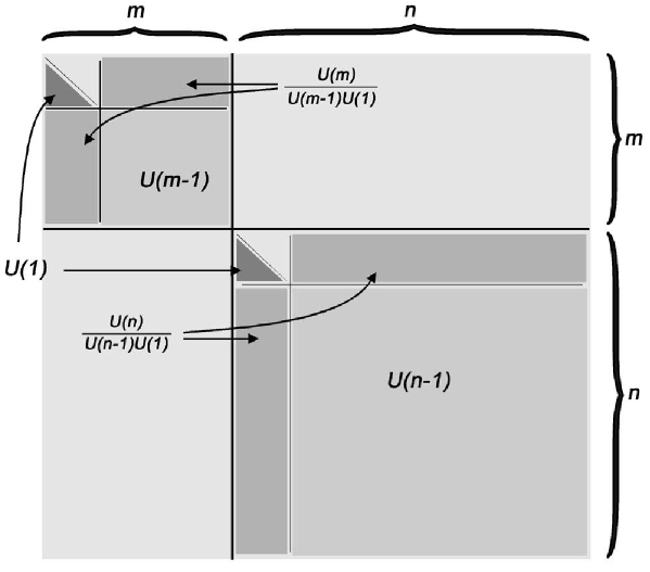
Figure 7: Symmetry breaking.

From this one can see that besides the scale size $\lambda$ and position $z_{0}$ the instanton manifold is spanned by the $t^{\alpha\beta}_{1,-1}$ and $t^{\alpha\beta}_{-1,1}$ which are the generators of $U(m+n)/U(m)\times U(n)$. The $t^{1\alpha}_{1,1}$ and $t^{\alpha 1}_{1,1}$ with $\alpha>1$ are the generators of $U(n)/U(n-1)\times U(1)$ and the $t^{1\alpha}_{-1,-1}$ and $t^{\alpha 1}_{-1,-1}$ those of $U(m)/U(m-1)\times U(1)$. Finally, $t_{1,1}^{11}-t_{-1,-1}^{11}$ is the $U(1)$ generator describing the rotation of the $O(3)$ instanton about the $z$ axis. In total we find $2(mn+m+n)$ zero modes as it should be. The hierarchy of symmetry breaking by the one-instanton solution is illustrated in Fig. 7.

4.2 Spatially varying masses

We have seen that the quantum fluctuations about the instanton acquire the metric of a sphere, Eq. (92). This, however, complicates the problem of mass terms which are naturally written in flat space. To deal with this problem we modify the definition of the mass terms and introduce a spatially varying momentum scale $\mu(\textbf{r})$ as follows

$$z_{i}\rightarrow z_{i}\,\mu^{2}(\textbf{r}),$$ (113)

such that the action now becomes finite and can be written as

$$S_{i}=z_{i}\int d\textbf{r}\,O_{i}[Q]\rightarrow z_{i}\int d\textbf{r}\,\mu^{2}(\textbf{r})O_{i}[Q].$$ (114)

Several comments are in order. First of all, we expect that the introduction of a spatially varying momentum scale $\mu(\textbf{r})$ does not alter the singularity structure of the theory at short distances. We shall therefore proceed and first develop a full quantum theory for the modified mass terms in Sections  LABEL:@@ and  LABEL:@@. Secondly, we postpone the problem of curved versus flat space all the way until the end of the computation in Section @@ where we elaborate on the tricks developed by ’t Hooft.

As we shall discuss in detail in the remainder of this paper, the validity of the procedure with spatially varying masses relies entirely on the statement which says that the quantum theory of the modified instanton problem displays exactly the same ultraviolet singularities as those obtained in ordinary perturbative expansions. In fact, we shall greatly benefit from our introduction of observable parameters since it can be used to explicitly verify this statement.

Since the action is now finite one can go ahead and formally expand the theory about $z_{i}=0$. To see how this works let us first consider the operator $O_{h}$. Using Eq. (85) we can write for $S_{h}$

$$S_{h}=z_{h}\int d\textbf{r}\,\mu^{2}(\textbf{r})\mathop{\rm tr}\nolimits A_{h}q,$$ (115)

where

$$A_{h}=R\,T_{0}\left(\Lambda-\frac{m-n}{m+n}1_{m+n}\right)T^{-1}_{0}R^{-1}.$$ (116)

We can now proceed by evaluating the expectation $\langle q\rangle$ with respect to the theory of the previous Section, Eq. (90). The details of the computation are presented in Appendix B. It is important to keep in mind, however, that the global unitary matrix $T_{0}$ is eventually restricted to run over the subgroup $U(m)\times U(n)$ only. Since it is in many ways simpler to carry out the quantum fluctuations about the theory with $T_{0}=1_{m+n}$, we shall in what follows specialize to this simpler case. We will come back to the more general situation in Section  LABEL:@@ where we show that the final results are in fact independent of the specific choice made for the matrix $T_{0}$.

4.3 Action for the quantum fluctuations

Keeping the remarks of the previous Section in mind we obtain the complete action as the sum of a classical part $S^{\rm inst}$ and a quantum part $\delta S$ as follows

$$S=S^{\rm inst}+\delta S,$$ (117)

where

$$S^{\rm inst}=-2\pi\sigma_{xx}+i\,\theta+S^{\rm inst}_{h}+S^{\rm inst}_{a}+S^{\rm inst}_{s}$$ (118)

and

$$\delta S=\delta S_{\sigma}+\delta S_{h}+\delta S_{a}+\delta S_{s}.$$ (119)

Here, $S^{\rm inst}_{i}$ stands for the classical action of the modified mass terms $O_{i}^{\rm inst}$, Eq. (57), and is given by

$$S_{h}^{\rm inst} = z_{h}\int d\textbf{r}\,\mu^{2}(\textbf{r})O_{h}^{\rm inst}(\textbf{r})=-8\pi z_{h},$$

$$S_{a}^{\rm inst} = z_{a}\int d\textbf{r}\,\mu^{2}(\textbf{r})O_{a}^{\rm inst}(\textbf{r})=16\pi(m+n-1)z_{a},$$ (120)

$$S_{s}^{\rm inst} = z_{s}\int d\textbf{r}\,\mu^{2}(\textbf{r})O_{s}^{\rm inst}(\textbf{r})=16\pi(m+n+1)z_{s}\left[1-\frac{8}{3(m+n+2)}\right].$$

Next, the results for $\delta S_{\sigma}$ and $\delta S_{i}$ can be written up to quadratic order in $v$, $v^{\dagger}$ as follows

$$\delta S_{\sigma}=-\frac{\sigma_{xx}}{4}\int\limits_{\eta\theta}\Biggl{[}\sum\limits_{\alpha=2}^{m}\sum\limits_{\beta=2}^{n}v^{\alpha\beta}O^{(0)}v^{{\dagger}\beta\alpha}+\sum\limits_{\alpha=2}^{m}v^{\alpha 1}O^{(1)}v^{{\dagger}1\alpha}+\sum\limits_{\beta=2}^{n}v^{1\beta}O^{(1)}v^{{\dagger}\beta 1}$$

$$+v^{11}O^{(2)}v^{{\dagger}11}\Biggr{]}$$ (121)

The operators $O^{(a)}$ with $a=0,1,2$ are given by Eq. (97). Furthermore,

$$\delta S_{h}=-z_{h}\int\limits_{\eta\theta}\Biggl{[}\sum\limits_{\alpha=2}^{m}\sum\limits_{\beta=2}^{n}v^{\alpha\beta}v^{{\dagger}\beta\alpha}+(1-e_{0}^{2})\left(\sum\limits_{\alpha=2}^{m}v^{\alpha 1}v^{{\dagger}1\alpha}+\sum\limits_{\beta=2}^{n}v^{1\beta}v^{{\dagger}\beta 1}\right)$$

$$+(1-2e_{0}^{2})v^{11}v^{{\dagger}11}+2(e_{0}e_{1}v^{11}+e_{0}\bar{e}_{1}v^{{\dagger}11})\Biggr{]},$$ (122)

$$\delta S_{a}=2(m+n-1)z_{a}\int\limits_{\eta\theta}\Biggl{[}\frac{m+n-2-4e_{0}^{2}}{m+n-2}\sum\limits_{\alpha=2}^{m}\sum\limits_{\beta=2}^{n}v^{\alpha\beta}v^{{\dagger}\beta\alpha}+(1-e_{0}^{2})$$

$$\hskip 142.26378pt\times\Bigl{(}\sum\limits_{\alpha=2}^{m}v^{\alpha 1}v^{{\dagger}1\alpha}+\sum\limits_{\beta=2}^{n}v^{1\beta}v^{{\dagger}\beta 1}\Bigr{)}+(1-2e_{0}^{2})v^{11}v^{{\dagger}11}$$

$$\hskip 22.76228pt+2(e_{0}e_{1}v^{11}+e_{0}\bar{e}_{1}v^{{\dagger}11})\Biggr{]},$$ (123)

$$\delta S_{s}=2\frac{m+n+1}{m+n+2}z_{s}\int\limits_{\eta\theta}\Biggl{[}(m+n+2-4e_{0}^{2})\sum\limits_{\alpha=2}^{m}\sum\limits_{\beta=2}^{n}v^{\alpha\beta}v^{{\dagger}\beta\alpha}+(1-e_{0}^{2})$$

$$\hskip 128.0374pt\times(m+n+2-8e_{0}^{2})\left(\sum\limits_{\alpha=2}^{m}v^{\alpha 1}v^{{\dagger}1\alpha}+\sum\limits_{\beta=2}^{n}v^{1\beta}v^{{\dagger}\beta 1}\right)$$

$$\hskip 128.0374pt+\Bigl{[}(1-2e_{0}^{2})(m+n+2-8e_{0}^{2})-8e_{0}^{2}|e_{1}|^{2}\Bigr{]}v^{11}v^{{\dagger}11}$$

$$\hskip 31.2982pt-4(e_{0}^{2}e_{1}^{2}v^{11}v^{11}+e_{0}^{2}\bar{e}_{1}^{2}v^{{\dagger}11}v^{{\dagger}11})$$

$$\hskip 125.19194pt+2(m+n+2-8e_{0}^{2})(e_{0}e_{1}v^{11}+e_{0}\bar{e}_{1}v^{{\dagger}11})\Biggr{]}.$$ (124)

Notice that the terms linear in $v$, $v^{\dagger}$ in Eqs (122)-(124) can be written as

$$\int\limits_{\eta\theta}\left[e_{0}e_{1}v^{11}+e_{0}\bar{e}_{1}v^{{\dagger}11}\right]\propto\int\limits_{\eta\theta}\left[\Phi^{(2)}_{1,-1}v^{11}+\bar{\Phi}^{(2)}_{1,-1}v^{{\dagger}11}\right]\propto\frac{\delta\lambda}{\lambda}.$$ (125)

This means that the fluctuations tangential to the instanton parameter $\lambda$ are the only unstable fluctuations in the problem. However, the linear fluctuations are not of any special interest to us and we proceed by formally evaluating the quantum fluctuations to first order in the fields $z_{i}$ only. The expansion is therefore with respect to the theory with $\delta S_{\sigma}$ alone and this has been analyzed in detail in Ref.[21, 22].

Finally, we also need the action $S^{0}$ for the quantum fluctuations about the trivial vacuum. The result is given by

$$S^{(0)}=\delta S_{\sigma}^{(0)}+\delta S_{h}^{(0)}+\delta S_{a}^{(0)}+\delta S_{s}^{(0)}$$ (126)

where

$$\delta S_{\sigma}^{(0)}=-\frac{\sigma_{xx}}{4}\int\limits_{\eta\theta}\sum\limits_{\alpha=1}^{m}\sum\limits_{\beta=1}^{n}v^{\alpha\beta}O^{(0)}v^{{\dagger}\beta\alpha},\qquad\delta S_{h}^{(0)}=-z_{h}\int\limits_{\eta\theta}\sum\limits_{\alpha=1}^{m}\sum\limits_{\beta=1}^{n}v^{\alpha\beta}v^{{\dagger}\beta\alpha},$$

$$\delta S_{a,s}^{(0)}=2(m+n\mp 1)z_{a,s}\int\limits_{\eta\theta}\sum\limits_{\alpha=1}^{m}\sum\limits_{\beta=1}^{n}v^{\alpha\beta}v^{{\dagger}\beta\alpha}.$$ (127)

5 Pauli-Villars regulators

Recall that after integration over the quantum fluctuations one is left with two sources of divergences. First, there are the ultraviolet divergences which eventually lead to the renormalization of the coupling constant or $\sigma_{xx}$. At present we wish to extend the analysis to include the renormalization of the the $z_{i}$ fields. The ultraviolet can be dealt with in a standard manner, employing Pauli-Villars regulator fields with masses ${\mathcal{M}}_{f}$ ($f=0,1,\cdots,K$) and with an alternating metric $\hat{e}_{f}$ [28]. We assume $\hat{e}_{0}=1$, ${\mathcal{M}}_{0}=0$ and large masses $\mathcal{M}_{f}\gg 1$ for $f>1$. The following constraints are imposed

$$\sum\limits_{f=0}^{K}\hat{e}_{f}\mathcal{M}^{k}_{f}=0,\qquad 0\leq k<K,\qquad\sum\limits_{f=1}^{K}\hat{e}_{f}\ln{\mathcal{M}}_{f}=-\ln{\mathcal{M}}.$$

The regularized theory is then defined as

$$\delta S_{\rm reg}=\delta S_{0}+\sum\limits_{f=1}^{K}\hat{e}_{f}\delta S_{f}.$$ (128)

Here action $\delta S_{f}$ is the same as the action $\delta S$ except that the kinetic operators $O^{(a)}$ are all replaced by $O^{(a)}+{\mathcal{M}}_{f}^{2}$.

Our task is to evaluate Eq. (128) to first order in the fields $z_{i}$. This means that $\delta S_{0}$ still naively diverges due to the zero modes of the operators $O^{(a)}$. These zero modes are handled separately in Section 6, by employing the collective coordinate formalism introduced in Ref.[21]. The regularized theory $\delta S_{\rm reg}$ is therefore defined by omitting the contributions of all the zero modes in $\delta S_{0}$.

To simplify the notation we shall work with $m=n$ in the subsequent Sections. The final answer will be expressed in terms of $m$ and $n$, however.

5.1 Explicit computations

To simplify the notation we will first collect the results obtained after a naive integration over the field variables $v,v^{\dagger}$. These are easily extended to include the alternating metric and the Pauli-Villars masses which will be main topic of the next Section. Consider the ratio

$$\frac{Z_{\rm inst}}{Z_{0}}=\frac{\displaystyle\int\mathcal{D}[v,v^{\dagger}]\exp S}{\displaystyle\int\mathcal{D}[v,v^{\dagger}]\exp S_{0}}=\exp\Bigl{[} - 2\pi\sigma_{xx}\pm i\theta+D$$ (129)

$$+ S_{h}^{\rm inst}+\Delta S_{h}$$

$$+ S_{a}^{\rm inst}+\Delta S_{a}$$

$$+ S_{s}^{\rm inst}+\Delta S_{s}\Bigr{]}.$$

Here, the quantum corrections $D$, $\Delta S_{h}$, $\Delta S_{a}$ and $\Delta S_{s}$ can be expressed in terms of the propagators

$$\mathcal{G}_{a}=\frac{1}{O^{(a)}}=\sum\limits_{JM}\frac{|JM\rangle_{(a)}{}_{(a)}\langle JM|}{E_{J}^{(a)}},\qquad a=0,1,2.$$ (130)

The results can be written as follows

$$D = \mathop{\rm tr}\nolimits\left[2(n-1)\Bigl{(}\ln\mathcal{G}_{1}-\ln\mathcal{G}_{0}\Bigr{)}-\Bigl{(}\ln\mathcal{G}_{2}-\ln\mathcal{G}_{0}\Bigr{)}\right],$$ (131)

$$\Delta S_{h} = -\frac{4z_{h}}{\sigma_{xx}}\mathop{\rm tr}\nolimits\Bigl{[}2(n-1)[(1-e_{0}^{2})\mathcal{G}_{1}-\mathcal{G}_{0}]+[(1-2e_{0}^{2})\mathcal{G}_{2}-\mathcal{G}_{0}]\Bigr{]},$$ (132)

$$\Delta S_{a} = \frac{8(2n-1)z_{a}}{\sigma_{xx}}\mathop{\rm tr}\nolimits\Bigl{[}(n-1)[(n-1-2e_{0}^{2})\mathcal{G}_{0}-(n-1)\mathcal{G}_{0}]$$

$$\hskip 71.13188pt+2(n-1)[(1-e_{0}^{2})\mathcal{G}_{1}-\mathcal{G}_{0}]+[(1-2e_{0}^{2})\mathcal{G}_{2}-\mathcal{G}_{0}]\Bigr{]},$$

$$\Delta S_{s} = \frac{8(2n+1)z_{s}}{(n+1)\sigma_{xx}}\mathop{\rm tr}\nolimits\Bigl{[}(n-1)^{2}[(n+1-2e_{0}^{2})\mathcal{G}_{0}-(n+1)\mathcal{G}_{0}]$$

$$\hskip 71.13188pt+2(n-1)[(1-e_{0}^{2})(n+1-4e_{0}^{2})\mathcal{G}_{1}-(n+1)\mathcal{G}_{0}]$$

$$\hskip 71.13188pt+\Bigl{(}[(1-2e_{0}^{2})(n+1-4e_{0}^{2})-4e_{0}^{2}(1-e_{0}^{2})]\mathcal{G}_{2}$$

$$\hskip 71.13188pt-(n+1)\mathcal{G}_{0}\Bigr{)}\Bigr{]}.$$

In these expressions the trace is taken with respect to the complete set of eigenfunctions of the operators $O^{(a)}$. To evaluate these expressions we need the help of the following identities (see Appendix C)

$$\sum\limits_{M=-J-a+k_{a}}^{J-k_{a}}{}_{(a)}\langle J,M|e_{0}^{2}|M,J\rangle_{(a)}=\frac{1}{2}(2J+1+a-2k_{a}),$$ (135)

$$\sum\limits_{M=-J-a+k_{a}}^{J-k_{a}}{}_{(a)}\langle J,M|e_{0}^{4}|M,J\rangle_{(a)}=\frac{1}{3}(2J+1+a-2k_{a}),$$ (136)

where $k_{a}={0,1,1}$ for $a=0,1,2$ respectively. After elementary algebra we obtain

$$D = -2(n-1)D^{(1)}-D^{(2)},$$ (137)

$$\Delta S_{h} = \hskip 62.88077pt-z_{h}\frac{4}{\sigma_{xx}}\left[(n-1)Y^{(1)}-(2n-1)Y^{(0)}\right],$$ (138)

$$\Delta S_{a} = \hskip 41.25641ptz_{a}\frac{8(2n-1)}{\sigma_{xx}}\left[(n-1)Y^{(1)}-(3n-2)Y^{(0)}\right],$$ (139)

$$\Delta S_{s} = z_{s}\frac{8(2n+1)(3n-1)}{3(n+1)\sigma_{xx}}\left[(n-1)Y^{(1)}-3nY^{(0)}\right].$$ (140)

We have introduced the following quantities

$$D^{(r)} = \sum\limits_{J=1}^{\infty}(2J+r-1)\ln E_{J}^{(r)}-\sum\limits_{J=0}^{\infty}(2J+1)\ln E_{J}^{(0)},~{}~{}~{}r=1,2$$ (141)

$$Y^{(s)} = \sum\limits_{J=s}^{\infty}\frac{2J+1-s}{E^{(s)}_{J}},\qquad s=0,1.$$ (142)

5.2 Regularized expressions

To obtain the regularized theory one has to include the alternating metric $e_{f}$ and add the masses $\mathcal{M}_{f}$ to the energies $E_{J}^{(a)}$ in the expressions for $D^{(r)}$ and $Y^{(s)}$. To start, let us define the function

$$\Phi^{(\Lambda)}(p)=\sum\limits_{J=p}^{\Lambda}2J\ln(J^{2}-p^{2}).$$ (143)

According to Eq. (128), the regularized function $\Phi^{(\Lambda)}_{\rm reg}(p)$ is given by

$$\Phi^{(\Lambda)}_{\rm reg}(p)=\sum\limits_{J=p+1}^{\Lambda}2J\ln(J^{2}-p^{2})+\sum\limits_{f=1}^{K}e_{f}\sum\limits_{J=p}^{\Lambda}2J\ln(J^{2}-p^{2}+{\mathcal{M}}^{2}_{f}),$$ (144)

where we assume that the cut-off $\Lambda$ is much larger than $\mathcal{M}_{f}$. In the presence of a large mass $\mathcal{M}_{f}$ we may consider the logarithm to be a slowly varying function of the discrete variable $J$. We may therefore approximate the summation by using the Euler-Maclaurin formula

$$\sum\limits_{J=p+1}^{\Lambda}g(J)=\int\limits_{p}^{\Lambda}g(x)dx+\frac{1}{2}g(x)\Bigr{|}_{p}^{\Lambda}+\frac{1}{12}g^{\prime}(x)\Bigr{|}_{p}^{\Lambda}.$$ (145)

After some algebra we find that Eq. (144) can be written as follows [21]

$$\Phi^{(\Lambda)}_{\rm reg}(p)=-2\Lambda(\Lambda+1)\ln\Lambda+\Lambda^{2}-\frac{\ln e\Lambda}{3}+4\sum\limits_{J=1}^{\Lambda}J\ln J$$

$$+\frac{1-6p}{3}\ln{\mathcal{M}}+2p^{2}-2\sum\limits_{J=1}^{2p}(J-p)\ln J.$$ (146)

The regularized expression for $D^{(r)}$ can be obtained as

$$D^{(r)}_{\rm reg}=\lim\limits_{\Lambda\to\infty}\left[\Phi^{(\Lambda)}_{\rm reg}\left(\frac{1+r}{2}\right)-\Phi^{(\Lambda)}_{\rm reg}\left(\frac{1}{2}\right)\right].$$ (147)

From this we obtain the final results

$$D^{(1)}_{\rm reg}=-\ln\mathcal{M}+\frac{3}{2}-2\ln 2,\qquad D^{(2)}_{\rm reg}=-2\ln\mathcal{M}+4-3\ln 3-\ln 2.$$ (148)

Next, we introduce another function

$$Y^{(\Lambda)}(p)=\sum\limits_{J=p}^{\Lambda}\frac{2J}{J^{2}-p^{2}},$$ (149)

According to Eq. (128), the regularized function $Y^{(\Lambda)}_{\rm reg}(p)$ is given by

$$Y^{(\Lambda)}_{\rm reg}(p)=\sum\limits_{f=1}^{K}e_{f}\sum\limits_{J=p}^{\Lambda}\frac{2J}{J^{2}-p^{2}+{\mathcal{M}}^{2}_{f}}+\sum\limits_{J=p+1}^{\Lambda}\frac{2J}{J^{2}-p^{2}},$$ (150)

where as before we assume that the cut-off $\Lambda\gg\mathcal{M}_{f}$. By using a similar procedure as discussed above we now find

$$Y^{(\Lambda)}_{\rm reg}(p)=2\ln\mathcal{M}+2\gamma-\sum\limits_{J=1}^{2p}\frac{1}{J}.$$ (151)

The regularized expressions for $Y^{(s)}$ can be written as

$$Y^{(s)}_{\rm reg}=\lim\limits_{\Lambda\to\infty}Y^{(\Lambda)}_{\rm reg}\left(\frac{1+s}{2}\right),$$ (152)

such that we finally obtain

$$Y^{(0)}_{\rm reg}=2\ln\mathcal{M}+2\gamma-1,\qquad Y^{(1)}_{\rm reg}=2\ln\mathcal{M}+2\gamma-\frac{3}{2}.$$ (153)

We therefore have the following results for the quantum corrections

$$D^{\rm reg} = 2n\ln\mathcal{M}+n(4\ln 2-3)-1+3\ln\frac{3}{2},$$ (154)

$$\Delta S_{h}^{\rm reg} = \hskip 92.75581ptz_{h}\frac{8n}{\sigma_{xx}}\left[\ln\mathcal{M}e^{\gamma-1/2}-\frac{2n-1}{4n}\right],$$ (155)

$$\Delta S_{a}^{\rm reg} = \hskip 42.10995pt-z_{a}\frac{16(2n-1)^{2}}{\sigma_{xx}}\left[\ln\mathcal{M}e^{\gamma-1/2}-\frac{3n-2}{2(2n-1)}\right],$$ (156)

$$\Delta S_{s}^{\rm reg} = -z_{s}\frac{16(2n+1)^{2}(3n-1)}{3\sigma_{xx}(n+1)}\left[\ln\mathcal{M}e^{\gamma-1/2}-\frac{3n}{2(2n+1)}\right].$$ (157)

Apart from the logarithmic singularity in $\mathcal{M}$, the numerical constants in the expression for $D^{\rm reg}$ are going to play an important role in what follows. This is unlike the expressions for $\Delta S_{a}^{\rm reg}$ where the second term in the brackets should actually be considered as higher order terms in an expansion in powers of $1/\sigma_{xx}$. We collect the various terms together and obtain the following result for the instanton contribution to the free energy

$$\ln\left[\frac{Z_{\rm inst}}{Z_{0}}\right]^{\rm reg}=-1+3\ln\frac{3}{2} - (m+n)\left(\gamma+\frac{3}{2}-2\ln 2\right)\pm i\,\theta$$ (158)

$$-2\pi \sigma_{xx} \left[1-\frac{m+n}{2\pi\sigma_{xx}}\ln\mathcal{M}e^{\gamma}\right]$$ (159)

$$-8\pi z_{h} \left[1-\frac{m+n}{2\pi\sigma_{xx}}\ln\mathcal{M}e^{\gamma-1/2}\right]$$ (160)

$$+16\pi(m+n-1) z_{a} \left[1-\frac{m+n-1}{\pi\sigma_{xx}}\ln\mathcal{M}e^{\gamma-1/2}\right]$$ (161)

$$+\frac{16\pi(m+n+1)(3m+3n-2)}{3(m+n+2)} z_{s} \left[1-\frac{m+n+1}{\pi\sigma_{xx}}\ln\mathcal{M}e^{\gamma-1/2}\right].$$ (162)

5.3 Observable theory in Pauli Villars regularization

The important feature of these last expressions, as we shall see next, is that the quantum corrections to the parameters $\sigma_{xx}$, $z_{h}$, $z_{a}$ and $z_{a}$ are all identically the same as those obtained from the perturbative expansions of the observable parameters $\sigma^{\prime}_{xx}$, $z^{\prime}_{h}$, $z^{\prime}_{a}$ and $z^{\prime}_{a}$ introduced in Section 2.4. Notice that we have already evaluated this theory in dimensional regularization in Appendix B. The problem, however, is that the different regularization schemes (dimensional versus Pauli Villars) are not related to one another in any obvious fashion. Unlike dimensional regularization, for example, it is far from trivial to see how the general form of the observable parameters, Eq. (46), can be obtained from the theory in Pauli Villars regularization.

In Appendix D we give the details of the computation using Pauli-Villars regulators. Denoting the results for $\sigma_{xx}^{\prime}$ and $z_{i}^{\prime}$ by $\sigma_{xx}(\mathcal{M})$ and $z_{i}(\mathcal{M})$ respectively,

$$\sigma_{xx}^{\prime}=\sigma_{xx}(\mathcal{M}),~{}~{}~{}z_{i}^{\prime}=z_{i}(\mathcal{M})$$ (163)

then we have

$$\hskip 85.35826pt\sigma_{xx}(\mathcal{M}) = \sigma_{xx}\left[1-\frac{m+n}{2\pi\sigma_{xx}}\ln\mathcal{M}e^{\gamma}\right],$$ (164)

$$z_{i}(\mathcal{M}) = \hskip 7.11317ptz_{i}\left[1+\frac{\gamma_{i}^{(0)}}{\sigma_{xx}}\ln\mathcal{M}e^{\gamma-1/2}\right].$$ (165)

The coefficients $\gamma_{i}^{(0)}$ are given by

$$\gamma_{h}^{(0)}=-\frac{m+n}{2\pi},\qquad\gamma_{a}^{(0)}=-\frac{m+n-1}{\pi},\qquad\gamma_{s}^{(0)}=-\frac{m+n+1}{\pi}.$$ (166)

Since so much of what follows is based on the results obtained in this Section and the previous one, it is worthwhile to first present a summary of the various issues that are involved.
First of all, it is important to emphasize that our results for observable parameter $\sigma_{xx}^{\prime}$, Eq. (164), resolve an ambiguity that is well known to exist, in the instanton analysis of scale invariant theories. Given Eq. (164) one uniquely fixes the quantity $\sigma_{xx}(\mathcal{M})$ (Eq. 159) and the constant term of order unity (Eq. 158) that is otherwise left undetermined. This result becomes particularly significant when we address the non-perturbative aspects of the renormalization group $\beta$ functions in Section 7.
Secondly, the results for $z_{i}$ in the observable theory, Eq. 165), explicitly shows that the idea of spatially varying masses does not alter the ultraviolet singularity structure of the the instanton theory, i.e. Eqs 160 - 162. A deeper understanding of this problem is provided by the computations in Appendix D where we show that Pauli-Villars regularization retains translational invariance in the sense that the expectation of local operators like $<O_{i}\left(Q(r)\right)>$ is independent of $r$. This aspect of the problem is especially meaningful when dealing with the problem of electron-electron interactions. As is well known, the presence of mass terms generally alters the renormalization of the theory at short distances in this case, i.e. the renormalization group $\beta$ functions [9].
Finally, on the basis of the theory of observable parameters Eqs  (164) and (165) we may summarize the results of our instanton computation, Eqs  (158)-(162), as follows

$$\ln\left[\frac{Z_{\rm inst}}{Z_{0}}\right]^{\rm reg}= - 1+3\ln\frac{3}{2}-(m+n)\left(\gamma+\frac{3}{2}-2\ln 2\right)$$ (167)

$$- 2\pi\sigma_{xx}(\mathcal{M})\pm\,i\theta(\nu)$$ (168)

$$+ ~{}~{}~{}~{}~{}z_{h}(\mathcal{M})\int d\textbf{r}\mu^{2}(\textbf{r})O_{h}^{\rm inst}(\textbf{r})$$ (169)

$$+ ~{}~{}~{}~{}~{}z_{s}(\mathcal{M})\int d\textbf{r}\mu^{2}(\textbf{r})O_{s}^{\rm inst}(\textbf{r})$$ (170)

$$+ ~{}~{}~{}~{}~{}z_{a}(\mathcal{M})\int d\textbf{r}\mu^{2}(\textbf{r})O_{a}^{\rm inst}(\textbf{r}).$$ (171)

Here, the quantities $O_{i}^{\rm inst}(\textbf{r})$ are the classical expressions given by Eq.(59). On the other hand, the parameters $\sigma_{xx}(\mathcal{M})$ and $z_{i}(\mathcal{M})$ are precisely those obtained from the observable theory.

6 Instanton manifold

In this Section we first recapitulate the integration over the zero frequency modes following Refs [21] and [22]. In the second part of this Section we address the zero modes describing the $U(m+n)/U(m)\times U(n)$ rotation of the instanton that we sofar have discarded.

6.1 Zero frequency modes

The complete expression for ${Z_{\rm inst}}/{Z_{0}}$ can be written as follows

$$\frac{Z_{\rm inst}}{Z_{0}}=\frac{\int\mathcal{D}[Q_{\rm inst}]\left[Z_{\rm inst}\right]^{\rm reg}}{\int\mathcal{D}[Q_{0}]\left[Z_{0}\right]^{\rm reg}}.$$ (172)

Here, $Q_{\rm inst}$ denotes the manifold of the instanton parameters as is illustrated in Fig. 7

$$\int\mathcal{D}[Q_{\rm inst}] = A_{\rm inst}\int d\textbf{r}_{0}\int\frac{d\lambda}{\lambda^{3}}\int{\mathcal{D}}[U(1)]$$ (173)

$$\times \int{\mathcal{D}}\left[\frac{U(m)}{U(1)\times U(m-1)}\right]\int{\mathcal{D}}\left[\frac{U(n)}{U(1)\times U(n-1)}\right]$$

$$\times \int{\mathcal{D}}\left[\frac{U(m+n)}{U(m)\times U(n)}\right].$$

The $Q_{0}$ represents the zero modes associated with the trivial vacuum

$$\int\mathcal{D}[Q_{0}]=A_{0}\int{\mathcal{D}}\left[\frac{U(m+n)}{U(m)\times U(n)}\right].$$ (174)

The numerical factors $A_{\rm inst}$ and $A_{0}$ are given by

$$A_{\rm inst} = \langle e^{4}_{0}\rangle\langle|e_{1}|^{4}\rangle\langle e^{2}_{0}|e_{1}|^{2}\rangle\left(\langle e^{2}_{0}\rangle\langle|e_{1}|^{2}\rangle\right)^{m+n-2}\langle 1\rangle^{(m-1)(n-1)}\pi^{-mn-m-n}$$ (175)

$$A_{0} = \langle 1\rangle^{mn}\pi^{-mn}$$ (176)

where the average $\langle\cdots\rangle$ is with respect to the surface of a sphere

$$\langle f\rangle=\sigma_{xx}\int\limits_{-1}^{1}d\eta\int\limits_{0}^{2\pi}d\theta f(\eta,\theta).$$ (177)

Notice that in the absence of symmetry breaking terms the integration over $U(m+n)/U(m)\times U(n)$ drops out in the ratio. We shall first discard this integration in the final answer which is then followed by a justification in Section 6.2. With the help of the identity [21]

$$\int{\mathcal{D}}\left[\frac{U(k)}{U(1)\times U(k-1)}\right]=\frac{\pi^{k-1}}{\Gamma(k)},$$ (178)

we can write the complete result as follows

$$\frac{Z_{\rm inst}}{Z^{(0)}}=\frac{mn}{2}D_{mn}\int d\textbf{r}_{0}\int\frac{d\lambda}{\lambda^{3}}(2\pi\sigma_{xx})^{n+m}\exp S^{\prime}_{\rm inst}$$ (179)

where

$$S^{\prime}_{\rm inst}=-2\pi\sigma_{xx}({\mathcal{M}})\pm i\theta+z_{h}({\mathcal{M}})\int\limits_{\eta\theta}O_{h}^{\rm inst}+z_{s}({\mathcal{M}})\int\limits_{\eta\theta}O_{s}^{\rm inst}+z_{a}({\mathcal{M}})\int\limits_{\eta\theta}O_{a}^{\rm inst}.$$ (180)

The numerical constant $D_{mn}$ is given by

$$D_{mn}=\frac{4}{\pi e}e^{-(m+n)(\gamma+3/2-\ln 2)}\Gamma^{-1}(1+m)\Gamma^{-1}(1+n).$$ (181)

6.2 The $U(m+n)/U(m)\times U(n)$ zero modes

To justify the result of Eq. (179) we next consider the full expression for $Z_{\rm inst}/Z_{0}$ that includes the $U(m+n)/U(m)\times U(n)$ rotational degrees of freedom. For simplicity we limit ourselves to the theory in the presence of the $z_{h}$ field only. We now have

$$\frac{Z_{\rm inst}}{Z_{0}}=\frac{\int\mathcal{D}[Q_{\rm inst}]\exp\{-2\pi\sigma_{xx}\pm i\,\theta+z_{h}\int\limits_{\eta\theta}\mathop{\rm tr}\nolimits\Lambda_{h}T^{-1}_{0}\left[R^{-1}\langle q\rangle R\right]^{\rm reg}T_{0}\}}{\int\mathcal{D}[{Q}_{0}]\exp\{z_{h}\int\limits_{\eta\theta}\mathop{\rm tr}\nolimits\Lambda_{h}{t}^{-1}_{0}\left[\langle q\rangle_{0}\right]^{\rm reg}{t}_{0}\}}.$$ (182)

Here, we have defined

$$\Lambda_{h}=\Lambda-\frac{m-n}{m+n}1_{m+n}.$$ (183)

The expectation $\langle\cdots\rangle$ is with respect to the theory of $\delta S_{\sigma}$, Eq. (121), whereas $\langle\cdots\rangle_{0}$ refers to the quantum theory of the trivial vacuum which is obtained from $\delta S_{\sigma}$ by replacing all operators $O^{(a)}$ by $O^{(0)}$. Let us write the rotational degrees of freedom $T_{0}\in U(m+n)$ as follows

$$T_{0}=t_{0}W,\qquad Q_{0}=t_{0}^{-1}\Lambda t_{0}.$$ (184)

The quantity $t_{0}$ or $Q_{0}$ runs over the manifold $U(m+n)/U(m)\times U(n)$ and $W$ stands for the remaining degrees of freedom $U(m)/U(m-1)\times U(1)$, $U(n)/U(n-1)\times U(1)$ and $U(1)$ respectively. We can write

$$\int\mathcal{D}[Q_{\rm inst}]=A_{\rm inst}\int d\textbf{r}_{0}\frac{d\lambda}{\lambda^{3}}\mathcal{D}[Q_{0}]\mathcal{D}[W]$$ (185)

The quantity $\left[R^{-1}\langle q\rangle R\right]^{\rm reg}$, unlike $\left[\langle q\rangle_{0}\right]^{\rm reg}$ in Eq. (182), is not invariant under $U(m)\times U(n)$ rotations. We therefore perform the integration over $W$ explicitly as follows

$$\left\langle\exp\left[z_{h}\int\limits_{\eta\theta}\mathop{\rm tr}\nolimits\Lambda_{h}t^{-1}_{0}W^{-1}\left[R^{-1}\langle q\rangle R\right]^{\rm reg}Wt_{0}\right]\right\rangle_{W}\qquad\qquad{}$$ (186)

$${}\qquad\qquad\qquad=\exp\left[z_{h}\int\limits_{\eta\theta}\frac{O_{h}(Q_{0})}{O_{h}(\Lambda)}\mathop{\rm tr}\nolimits\Lambda_{h}\left[R^{-1}\langle q\rangle R\right]^{\rm reg}+\mathcal{O}(z_{h}^{2})\right].$$

Here,

$$\langle X[W]\rangle_{W}=\frac{\int\mathcal{D}[W]X[W]}{\int\mathcal{D}[W]}.$$ (187)

The $Q_{0}$ is now the only rotational degree of freedom left in the terms with $z_{h}$ and the result can therefore be written as follows

$$\frac{Z_{\rm inst}}{Z^{(0)}}=\frac{mn}{2}D_{mn}\int d\textbf{r}_{0}\int\frac{d\lambda}{\lambda^{3}}(2\pi\sigma_{xx})^{m+n}\exp\left[-2\pi\sigma_{xx}\pm i\,\theta+\delta S^{\prime}_{\rm inst}\right],$$ (188)

where

$$\exp\delta S^{\prime}_{\rm inst}=\frac{\int\mathcal{D}[Q_{0}]\exp\{z_{h}\int\limits_{\eta\theta}\frac{O_{h}(Q_{0})}{O_{h}(\Lambda)}\mathop{\rm tr}\nolimits\Lambda_{h}\left[R^{-1}\langle q\rangle R\right]^{\rm reg}\}}{\int\mathcal{D}[{Q}_{0}]\exp\{z_{h}\int\limits_{\eta\theta}\frac{O_{h}({Q}_{0})}{O_{h}(\Lambda)}\mathop{\rm tr}\nolimits\Lambda_{h}\left[\langle q\rangle_{0}\right]^{\rm reg}\}}.$$ (189)

We can write the result as an expectation with respect to the matrix field variable $Q_{0}$,

$$\exp\delta S^{\prime}_{\rm inst}=\left\langle\exp\{z_{h}\int\limits_{\eta\theta}\frac{O_{h}(Q_{0})}{O_{h}(\Lambda)}\mathop{\rm tr}\nolimits\Lambda_{h}\left[R^{-1}\langle q\rangle R-\langle q\rangle_{0}\right]^{\rm reg}\}\right\rangle_{Q_{0}},$$ (190)

where

$$\langle X[Q_{0}]\rangle_{Q_{0}}=\frac{\int\mathcal{D}[Q_{0}]\exp\{z_{h}\int\limits_{\eta\theta}\frac{O_{h}(Q_{0})}{O_{h}(\Lambda)}\mathop{\rm tr}\nolimits\Lambda_{h}\left[\langle q\rangle_{0}\right]^{\rm reg}\}X[Q_{0}]}{\int\mathcal{D}[{Q}_{0}]\exp\{z_{h}\int\limits_{\eta\theta}\frac{O_{h}({Q}_{0})}{O_{h}(\Lambda)}\mathop{\rm tr}\nolimits\Lambda_{h}\left[\langle q\rangle_{0}\right]^{\rm reg}\}}.$$ (191)

Notice that by putting the classical value $\langle q\rangle=\langle q\rangle_{0}=\Lambda$ in the expression $[\cdots]^{\rm reg}$ in Eq. (190) we precisely obtain the quantity $O_{h}^{\rm inst}$. We therefore identify (see also Eq. (180))

$$\int\limits_{\eta\theta}z_{h}\mathop{\rm tr}\nolimits\Lambda_{h}\left[R^{-1}\langle q\rangle R-\langle q\rangle_{0}\right]^{\rm reg}=\int\limits_{\eta\theta}z_{h}(\mathcal{M})O_{h}^{\rm inst}.$$ (192)

This is precisely the result that was obtained before, by fixing $Q_{0}=\Lambda$ at the outset. By the same token we write

$$z_{h}\mathop{\rm tr}\nolimits\Lambda_{h}\left[\langle q\rangle_{0}\right]^{\rm reg}=z_{h}(\mathcal{M})O_{h}(\Lambda)$$ (193)

We have already seen that the quantity $z_{h}(\mathcal{M})$ defined by Eq. (192) differs from that of Eq. (193) by a constant of order $1/\sigma_{xx}$ which is not of interest to us. The final expression for $\delta S^{\prime}_{\rm inst}$ can now be written in a more transparent fashion as follows

$$\exp\delta S^{\prime}_{\rm inst}=\left\langle\exp\left\{\frac{O_{h}(Q_{0})}{O_{h}(\Lambda)}\int\limits_{\eta\theta}z_{h}(\mathcal{M})O_{h}^{\rm inst}\right\}\right\rangle_{Q_{O}},$$ (194)

where instead of Eq. (191) we now write

$$\langle X[Q_{0}]\rangle_{Q_{0}}=\frac{\int\mathcal{D}[Q_{0}]\exp\{\int\limits_{\eta\theta}z_{h}(\mathcal{M}){O_{h}(Q_{0})}\}X[Q_{0}]}{\int\mathcal{D}[{Q}_{0}]\exp\{\int\limits_{\eta\theta}z_{h}(\mathcal{M})O_{h}({Q}_{0})\}}.$$ (195)

In summary we can say that as long as one works with mass terms in curved space, the rotational degrees of freedom are non-trivial and the integration over the global matrix field $Q_{0}$ has to be performed in accordance with Eq. (195). However, we are ultimately interested in the theory in flat space which means that the integral over the unit sphere $\int d\eta d\theta$ in Eq. (195) is going to be replaced by the integral over the entire plane in flat space, $\int d\textbf{r}$. This then fixes the matrix variable $Q_{0}$ in Eqs (LABEL:OmegaInstRes1) and (195) to its classical value $Q_{0}=\Lambda$. The final results are therefore the same as those that are obtained by putting $Q_{0}=\Lambda$ at the outset of the problem.

7 Transformation from curved space to flat space

In this Section we embark on the various steps that are needed in order express the final answer in quantities that are defined in flat space. As a first step we have undo the transformation $z_{i}\rightarrow z_{i}\mu^{2}({\bf r})$ that was introduced in Section 4.2 (see Eq. (113)). This means that the integrals over $\eta$, $\theta$ in the expression for $S^{\prime}_{\rm inst}$, Eq. (180), have to be replaced as follows

$$\int d\eta d\theta O_{i}^{\textrm{inst}}=\int d\textbf{r}\mu^{2}(\textbf{r})O_{i}^{\textrm{inst}}({\bf r})\quad\rightarrow\quad\int d\textbf{r}O_{i}^{\textrm{inst}}({\bf r}).$$ (196)

The complete expression for the instanton contribution to the free energy is therefore the same as Eq. (179) but with $S^{\prime}_{\rm inst}$ now given by

$$\hskip 85.35826ptS^{\prime}_{\rm inst}\quad\rightarrow\quad - 2\pi\sigma_{xx}({\mathcal{M}})\pm i\theta$$ (197)

$$+ \int^{\prime}d\textbf{r}z_{h}({\mathcal{M}})O_{h}^{\rm inst}(\textbf{r})$$ (198)

$$+ \int^{\prime}d\textbf{r}z_{s}({\mathcal{M}})O_{s}^{\rm inst}(\textbf{r})$$ (199)

$$+ \int^{\prime}d\textbf{r}z_{a}({\mathcal{M}})O_{a}^{\rm inst}(\textbf{r}).$$ (200)

The “prime” on the integral signs reminds us of the fact that the mass terms still formally display a logarithmic divergence in the infrared. However, from the discussion on constrained instantons we know that a finite value of $z_{i}$ generally induces an infrared cut-off on both the spatial integrals $\int d\textbf{r}O_{i}^{\rm inst}(\textbf{r})$ and the integral over scale sizes $\lambda$ in the theory. Keeping this in mind, we can proceed and evaluate the expressions for the physical observables of the theory, introduced in Section 2.4.

7.1 Physical observables

According to definitions in Section 2.4 we obtain the following results for the parameters $\sigma_{xx}^{\prime}$ and $\theta^{\prime}$ (see also Ref.  [21, 22])

$$\sigma_{xx}^{\prime} = \sigma_{xx}(\mathcal{M})-{D_{mn}}\int^{\prime}\frac{d\lambda}{\lambda}(2\pi\sigma_{xx})^{m+n+2}e^{-2\pi\sigma_{xx}(\mathcal{M})}\cos\theta$$ (201)

$$\frac{\theta^{\prime}}{2\pi} = \frac{\theta}{2\pi}\hskip 25.6073pt-D_{mn}\int^{\prime}\frac{d\lambda}{\lambda}(2\pi\sigma_{xx})^{m+n+2}e^{-2\pi\sigma_{xx}(\mathcal{M})}\sin\theta.$$ (202)

Similarly we obtain the $z^{\prime}_{i}$ parameters as follows

$$z_{i}^{\prime}=z_{i}(\mathcal{M})+D_{mn}\int^{\prime}\frac{d\lambda}{\lambda}(2\pi\sigma_{xx})^{m+n}e^{-2\pi\sigma_{xx}(\mathcal{M})}\cos\theta$$ (203)

$$\hskip 56.9055pt\times z_{i}(\mathcal{M})\left(\frac{mn}{O_{i}[\Lambda]}\int^{\prime}\frac{d\textbf{r}}{\lambda^{2}}O_{i}^{\rm inst}(\textbf{r})\right),$$

where $i=a,h$ and $s$. By using the results of Eqs (57) and (58), the expression simplifies somewhat and can be written in a more general fashion as follows

$$z_{i}^{\prime}=z_{i}(\mathcal{M})+\pi\gamma_{i}^{(0)}D_{mn}\int^{\prime}\frac{d\lambda}{\lambda}(2\pi\sigma_{xx})^{m+n}e^{-2\pi\sigma_{xx}(\mathcal{M})}\cos\theta$$ (204)

$$\hskip 56.9055pt\times z_{i}(\mathcal{M})\int^{\prime}d\textbf{r}\frac{\mu(\textbf{r})}{\lambda}.$$

The important feature of the results of this Section is that the non-perturbative (instanton) contributions are all unambiguously expressed in terms of the perturbative quantities $\sigma_{xx}({\mathcal{M}})$, $\theta$ and $z_{i}({\mathcal{M}})$.

7.2 Transformation  $\mu^{2}({\bf r}){\mathcal{M}}\rightarrow\mu_{0}$

Next we wish to obtain the results in terms of a spatially flat momentum scale $\mu_{0}$, rather than in the spatially varying quantity $\mu^{2}(\textbf{r})\mathcal{M}$ which appears in the Pauli-Villars regularization scheme. For this purpose we introduce the following renormalization group counter terms

$$\sigma_{xx}({\mathcal{M}})\rightarrow\sigma_{xx}({\mathcal{M}})\left[1+\frac{m+n}{2\pi\sigma_{xx}}\ln\frac{\mu(\textbf{r})\mathcal{M}}{\mu_{0}}\right]\hskip 113.81102pt{}$$ (205)

$$=\sigma_{xx}\left[1-\frac{m+n}{2\pi\sigma_{xx}}\ln\frac{\mu_{0}}{\mu(\textbf{r})}e^{\gamma}\right]=\sigma_{xx}(\mu(\textbf{r})),$$

$$z_{i}({\mathcal{M}})\rightarrow z_{i}({\mathcal{M}})\left[1+\frac{\gamma_{i}^{(0)}}{\sigma_{xx}}\ln\frac{\mu(\textbf{r}){\mathcal{M}}}{\mu_{0}}\right]\hskip 113.81102pt{}$$ (206)

$$=z_{i}\left[1-\frac{\gamma^{(0)}_{i}}{\sigma_{xx}}\ln\frac{\mu_{0}}{\mu(\textbf{r})}e^{\gamma-1/2}\right]=z_{i}(\mu(\textbf{r})).$$

The expression for $S^{\prime}_{\rm inst}$ now becomes

$$\hskip 71.13188ptS^{\prime}_{\rm inst}\quad\rightarrow\quad - \int d\textbf{r}\sigma_{xx}(\mu(\textbf{r}))\mathop{\rm tr}\nolimits(\nabla Q_{\rm inst}(\textbf{r}))^{2}\pm i\theta$$ (207)

$$+ \int^{\prime}d\textbf{r}z_{h}(\mu(\textbf{r}))O_{h}^{\rm inst}(\textbf{r})$$ (208)

$$+ \int^{\prime}d\textbf{r}z_{s}(\mu(\textbf{r}))O_{s}^{\rm inst}(\textbf{r})$$ (209)

$$+ \int^{\prime}d\textbf{r}z_{a}(\mu(\textbf{r}))O_{a}^{\rm inst}(\textbf{r}).$$ (210)

7.3 The $\beta$ functions

Let us first evaluate Eq. (207) which can be written as

$$\int d{\bf r}~{}\sigma_{xx}(\mu({\bf r}))\mathop{\rm tr}\nolimits\nabla_{i}Q_{\textrm{inst}}({\bf r})\nabla_{i}Q_{\textrm{inst}}({\bf r})=\int d{\bf r}\mu^{2}({\bf r})\sigma_{xx}(\mu({\bf r}))=2\pi\sigma_{xx}(\zeta\lambda),$$ (211)

where

$$\sigma_{xx}(\zeta\lambda)=\sigma_{xx}-\frac{m+n}{2\pi}\ln{\zeta\lambda\mu_{0}}e^{\gamma},\qquad\zeta=e^{2}/4.$$ (212)

Notice that the expression for $\sigma_{xx}(\zeta\lambda)$ can be simply obtained from $\sigma_{xx}({\mathcal{M}})$ by replacing the Pauli-Villars mass $\mathcal{M}$ according to

$${\mathcal{M}}\rightarrow\zeta\lambda\mu_{0}.$$ (213)

We next wish to express the quantity $\sigma_{xx}^{\prime}({\mathcal{M}})$ in a similar fashion. Write

$$\hskip 113.81102pt\sigma_{xx}^{\prime}({\mathcal{M}}) \rightarrow \sigma_{xx}^{\prime}(\mu^{\prime}({\bf r}))$$ (214)

$$\sigma_{xx}^{\prime}(\zeta\lambda^{\prime}) = \frac{1}{2\pi}\int d{\bf r}(\mu^{\prime}({\bf r}))^{2}\sigma_{xx}^{\prime}(\mu^{\prime}({\bf r})).$$ (215)

One can think of the $\mu^{\prime}({\bf r})=2\lambda^{\prime}/(r^{2}+\lambda^{\prime 2})$ as being a background instanton with a large scale size $\lambda^{\prime}$. The expressions for $\sigma_{xx}^{\prime}$ and $\theta^{\prime}$ in flat space can now be written as follows

$$\sigma_{xx}^{\prime}(\zeta\lambda^{\prime}) = \sigma_{xx}(\zeta\lambda^{\prime})-{D_{mn}}\int^{\prime}\frac{d\lambda}{\lambda}(2\pi\sigma_{xx})^{m+n+2}e^{-2\pi\sigma_{xx}(\zeta\lambda)}\cos\theta$$ (216)

$$\frac{\theta^{\prime}(\zeta\lambda^{\prime})}{2\pi} = ~{}\frac{\theta}{2\pi}\hskip 22.76228pt-{D_{mn}}\int^{\prime}\frac{d\lambda}{\lambda}(2\pi\sigma_{xx})^{m+n+2}e^{-2\pi\sigma_{xx}(\zeta\lambda)}\sin\theta.$$ (217)

In words, the scale size $\lambda^{\prime}$ has identically the same meaning for the perturbative and instanton contributions. Notice that $\sigma_{xx}(\zeta\lambda^{\prime})$ is the same as Eq. (212) with $\lambda$ replaced by $\lambda^{\prime}$. Next, introducing an arbitrary scale size $\lambda_{0}$ we can write the perturbative expression $\sigma_{xx}(\zeta\lambda_{0})$ as follows

$$\sigma_{xx}(\zeta\lambda^{\prime})=\sigma_{xx}(\zeta\lambda_{0})-\frac{m+n}{2\pi}\ln\frac{\lambda^{\prime}}{\lambda_{0}}=\sigma_{xx}(\zeta\lambda_{0})-\frac{m+n}{2\pi}\int_{\lambda_{0}}^{\prime}\frac{d\lambda}{\lambda}.$$ (218)

On the basis of these results one obtains the following complete expressions for the quantities $\sigma_{xx}^{\prime}$ and $\theta^{\prime}$

$$\sigma_{xx}^{\prime} = \sigma_{xx}(\zeta\lambda_{0})-\int^{\prime}_{\zeta\lambda_{0}}\frac{d[\zeta\lambda]}{\zeta\lambda}\left[\frac{m+n}{2\pi}+{D_{mn}}(2\pi\sigma_{xx})^{m+n+2}e^{-2\pi\sigma_{xx}(\zeta\lambda)}\cos\theta\right],$$

$$\frac{\theta^{\prime}}{2\pi} = ~{}\frac{\theta(\zeta\lambda_{0})}{2\pi}\hskip 5.12128pt-\int^{\prime}_{\zeta\lambda_{0}}\frac{d[\zeta\lambda]}{\zeta\lambda}{D_{mn}}(2\pi\sigma_{xx})^{m+n+2}e^{-2\pi\sigma_{xx}(\zeta\lambda)}\sin\theta.$$ (219)

Several remarks are in order. First of all, we have made use of the well known fact that the quantities $\sigma_{xx}$ in the integral over scale sizes all acquire the same quantum corrections and can be replaced by $\sigma_{xx}(\zeta\lambda)$. Secondly, although the instanton contributions are finite in the ultraviolet, they have nevertheless dramatic consequences for the behavior of the system in the infrared. Equations (220) and (219) determine the renormalization group $\beta$ functions as follows

$$\sigma_{xx}^{\prime} = \sigma_{xx}(\zeta\lambda_{0})-\int^{\prime}_{\zeta\lambda_{0}}\frac{d[\zeta\lambda]}{\zeta\lambda}\beta_{\sigma}(\sigma_{xx}(\zeta\lambda),\theta(\zeta\lambda))$$ (220)

$$\frac{\theta^{\prime}}{2\pi} = ~{}\frac{\theta(\zeta\lambda_{0})}{2\pi}\hskip 5.12128pt-\int^{\prime}_{\zeta\lambda_{0}}\frac{d[\zeta\lambda]}{\zeta\lambda}\beta_{\theta}(\sigma_{xx}(\zeta\lambda),\theta(\zeta\lambda))$$ (221)

where

$$\beta_{\sigma}(\sigma_{xx},\theta) = -\frac{d\sigma_{xx}}{d\ln\lambda}\hskip 13.08846pt=\frac{m+n}{2\pi}+{D_{mn}}(2\pi\sigma_{xx})^{m+n+2}e^{-2\pi\sigma_{xx}(\zeta\lambda)}\cos\theta,$$

$$\beta_{\theta}(\sigma_{xx},\theta) = -\frac{d(\theta/2\pi)}{d\ln\lambda}={D_{mn}}(2\pi\sigma_{xx})^{m+n+2}e^{-2\pi\sigma_{xx}(\zeta\lambda)}\sin\theta.$$ (222)

These final results which generalize those obtained earlier, on the basis of perturbative expansions (see Eq. (48)), are universal in the sense that they are independent of the particular regularization scheme that is being used to define the renormalized theory.

7.4 Negative anomalous dimension

Eqs (212), (213) and (215) provide a general prescription that should be used to translate the parameters $z_{i}({\mathcal{M}})$ and $z_{i}^{\prime}({\mathcal{M}})$ into the corresponding quantities $z_{i}({\zeta\lambda})$ and $z_{i}^{\prime}({\zeta\lambda^{\prime}})$ in flat space. Analogous to Eqs (211) and (215) we introduce the parameters $z_{i}$ and $z_{i}^{\prime}$ associated with scale sizes $\lambda$ and $\lambda^{\prime}$ respectively as follows

$$\hskip 85.35826ptz_{i}({\zeta\lambda}) = \frac{1}{2\pi}\int d{\bf r}\mu^{2}({\bf r})z_{i}(\mu({\bf r})),$$ (223)

$$z_{i}^{\prime}({\zeta\lambda^{\prime}}) = \frac{1}{2\pi}\int d{\bf r}(\mu^{\prime}({\bf r}))^{2}z_{i}(\mu({\bf r}).$$ (224)

Equation (223) implies that $z_{i}(\zeta\lambda)$ is related to $z_{i}({\mathcal{M}})$ according to the prescription of Eq. (213),

$$z_{i}(\zeta\lambda)=z_{i}\left[1-\frac{\gamma_{i}^{(0)}}{\sigma_{xx}}\ln{\zeta\lambda\mu_{0}}e^{\gamma-1/2}\right].$$ (225)

It is important to emphasize that the final expressions for $z_{i}({\zeta\lambda})$ and $\sigma_{xx}({\zeta\lambda})$ are consistent with those obtained in dimensional regularization (Appendix  A). Next we make use of Eqs (212), (223) and (224) and write the result for $z_{i}^{\prime}$, Eq. (204), as follows

$$z_{i}^{\prime}(\zeta\lambda^{\prime})=z_{i}(\zeta\lambda^{\prime})+D_{mn}\int^{\prime}\frac{d\lambda}{\lambda}(2\pi\sigma_{xx})^{m+n}e^{-2\pi\sigma_{xx}(\zeta\lambda)}{A}_{i}\cos\theta.$$ (226)

The problem that remains is to find the appropriate expression for the quantity $A_{i}$ which is defined as

$$A_{i}=\pi\gamma_{i}^{(0)}\int^{\prime}d\textbf{r}\frac{\mu(\textbf{r})}{\lambda}z_{i}({\mu(\textbf{r})}).$$ (227)

7.4.1 Amplitude $A_{i}$

To evaluate $A_{i}$ further it is convenient to introduce the quantity $M_{i}(\textbf{r})$ and write

$$A_{i}=-2\pi^{2}\gamma_{i}^{(0)}z_{i}(\mu(0))\int\limits_{\mu(0)}^{\mu(L^{\prime})}d[\ln\mu(\textbf{r})]M_{i}(\textbf{r}),\qquad M_{i}(\textbf{r})=\frac{z_{i}(\mu(\textbf{r}))}{z_{i}(\mu(0))}.$$ (228)

In the language of the Heisenberg ferromagnet $M_{i}(\textbf{r})$ represents a spatially varying spontaneous magnetization which is measured relative to the center $|\textbf{r}|=0$ of the instanton. Notice that for small instanton sizes $\lambda$ which are of interest to us, the associated momentum scale $\mu(\textbf{r})$ strongly varies from large values ${\mathcal{O}}(\lambda^{-1})$ at short distances ($|\textbf{r}|\ll\lambda$) to small values ${\mathcal{O}}(|\textbf{r}|^{-2})$ at very large distances ($|\textbf{r}|\gg\lambda$). Since a continuous symmetry cannot be spontaneously broken in two dimensions the results indicate that $M_{i}(\textbf{r})$ generally vanishes for large $|\textbf{r}|$. We therefore expect the amplitude $A_{i}$ to remain finite as $L^{\prime}\rightarrow\infty$. This is quite unlike the theory at a classical level where $A_{i}$ diverges and one is forced to work with the idea of constrained instantons.

Notice that the theory in the replica limit $m=n=0$ is in many ways special. In this case the anomalous dimension $\gamma_{i}$ of mass terms can have an arbitrary sign which means that $M_{a}(\textbf{r})$ can diverge as $|\textbf{r}|$ increases. In what follows we shall first deal with the problem of ordinary negative anomalous dimensions, including $\gamma_{i}=0$. This is then followed by an analysis of the special cases.

7.4.2 Details of computation

To simplify the discussion of the amplitude $A_{i}$ we limit ourselves to the theory with $\theta=0,\pi$ such that $\beta_{\theta}=0$ and $\beta_{\sigma}$, $\gamma_{i}$ are functions of $\sigma_{xx}$ only,

$$\gamma_{i}({\sigma_{xx}},\theta)\rightarrow\gamma_{i}({\sigma_{xx}}),\qquad\beta_{\sigma}({\sigma_{xx}},\theta)\rightarrow\beta_{\sigma}({\sigma_{xx}}).$$ (229)

Write

$$M_{i}(\textbf{r})=\exp\Bigl{\{}-\int\limits_{\ln\mu(0)}^{\ln\mu(\textbf{r})}d[\ln\mu]\gamma_{i}\Bigr{\}},$$ (230)

then the complete expression for $A_{i}$ becomes

$$A_{i}=-2\pi^{2}\gamma_{i}^{(0)}z_{i}(\mu(0))\int\limits_{\ln\mu(0)}^{\ln\mu(L^{\prime})}d[\ln\mu(\textbf{r})]\exp\Bigl{\{}-\int\limits_{\ln\mu(0)}^{\ln\mu(\textbf{r})}d[\ln\mu]\gamma_{i}\Bigr{\}}.$$ (231)

As a next step we change the integrals over $\ln\mu$ into integrals over $\sigma_{xx}$ and write

$$A_{i}=z_{i}(\mu(0)){\mathcal{H}}_{i}(\sigma_{xx}(\mu(0))),$$ (232)

where

$$\mathcal{H}_{i}=-2\pi^{2}\gamma_{i}^{(0)}\int\limits_{\sigma_{xx}(\mu(0))}^{\sigma_{xx}(\mu(L^{\prime}))}\frac{d\sigma_{xx}}{\beta_{\sigma}(\sigma_{xx})}\exp\Bigl{\{}-\int\limits_{\sigma_{xx}(\mu(0))}^{\sigma_{xx}}\frac{d\sigma}{\beta_{\sigma}(\sigma)}\gamma_{i}(\sigma)\Bigr{\}}.$$ (233)

The meaning of this result becomes more transparent if we write it in differential form. Taking the derivative of $\mathcal{H}_{i}$ with respect to $\ln\lambda$ we find

$$\left(\beta_{\sigma}(\sigma_{xx}(\mu(0)))\frac{d}{d\sigma_{xx}(\mu(0))}-\gamma_{i}(\sigma_{xx}(\mu(0)))\right)\mathcal{H}_{i}=2\pi^{2}\gamma^{(0)}_{i}\left(1+M_{i}(L^{\prime})\right).$$ (234)

Since in general we have $M_{i}(L^{\prime})\to 0$ for $\gamma^{(0)}_{i}<0$ we can safely put $L^{\prime}=\infty$ from now onward. At the same time one can solve Eq. (234) in the weak coupling limit $\lambda\to 0$ where $\mu(0)$, $\sigma_{xx}(\mu(0))\to\infty$. Under these circumstances it suffices to insert for $\gamma_{i}$ and $\beta_{\sigma}$ the perturbative expressions

$$\hskip 85.35826pt\gamma_{i}({\sigma_{xx}}) = \frac{\gamma_{i}^{(0)}}{\sigma_{xx}}+\mathcal{O}(\sigma_{xx}^{-2}),$$ (235)

$$\beta_{\sigma}({\sigma_{xx}}) = \beta_{0}+\frac{\beta_{1}}{\sigma_{xx}}+\mathcal{O}(\sigma_{xx}^{-2}),$$ (236)

where

$$\beta_{0}=\frac{m+n}{2\pi},\qquad\beta_{1}=\frac{mn+1}{2\pi^{2}}.$$ (237)

The differential equation becomes

$$\left(\beta_{0}+\frac{\beta_{1}}{\sigma_{xx}(\mu(0))}\right)\frac{d\mathcal{H}_{i}}{d\sigma_{xx}(\mu(0))}-\frac{\gamma_{i}^{(0)}}{\sigma_{xx}(\mu(0))}\mathcal{H}_{i}=2\pi^{2}\gamma^{(0)}_{i}.$$ (238)

The special solution can be written as follows

$$\mathcal{H}_{i}^{(1)}=\frac{2\pi^{2}\gamma_{i}^{(0)}}{\beta_{0}-\gamma_{i}^{(0)}}\left(\sigma_{xx}(\mu(0))+\frac{\beta_{1}}{\gamma_{i}^{(0)}}\right)$$ (239)

indicating that $\mathcal{H}_{i}$ can be written as a series expansion in powers of $1/\sigma_{xx}(\mu(0))$. The special solution $\mathcal{H}_{i}^{(1)}$ does not generally vanish when $\gamma_{i}^{(0)}\to 0$, however. To obtain the solution with the appropriate boundary conditions we need to solve the homogeneous equation. The result is

$$\mathcal{H}_{i}^{(0)}=C\left(1+\frac{\beta_{0}}{\beta_{1}}\sigma_{xx}(\mu(0))\right)^{\gamma_{i}^{(0)}/\beta_{0}}.$$ (240)

We obtain $\mathcal{H}_{i}=0$ for $\gamma_{i}^{(0)}=0$ provided we choose

$$C=-\frac{2\pi^{2}\gamma_{i}^{(0)}}{\beta_{0}-\gamma_{i}^{(0)}}\frac{\beta_{1}}{\gamma_{i}^{(0)}}.$$ (241)

The desired result for ${\mathcal{H}}_{i}(\sigma_{xx}(\mu(0)))$ therefore becomes

$${\mathcal{H}}_{i}=\frac{2\pi^{2}\gamma_{i}^{(0)}}{\beta_{0}-\gamma_{i}^{(0)}}\left\{\sigma_{xx}(\mu(0))+\frac{\beta_{1}}{\gamma_{i}^{(0)}}\left[1-\left(1+\frac{\beta_{0}}{\beta_{1}}\sigma_{xx}(\mu(0))\right)^{\gamma_{i}^{(0)}/\beta_{0}}\right]\right\}.$$ (242)

As a final step we next express $\sigma_{xx}(\mu(0))$ and $z_{i}(\mu(0))$ in terms of the flat space quantities $\sigma_{xx}(\zeta\lambda)$ and $z_{i}(\zeta\lambda)$ respectively. From the definitions of Eqs (212), (225), (205) and (206) we obtain the following relations

$$\hskip 85.35826pt\sigma_{xx}(\mu(0)) = \sigma_{xx}(\zeta\lambda)\left[1+\frac{\beta_{0}}{\sigma_{xx}(\zeta\lambda)}\ln 2\zeta\right],$$

$$z_{i}(\mu(0)) = \hskip 8.5359ptz_{i}(\zeta\lambda)\left[1+\frac{\gamma_{i}^{(0)}}{\sigma_{xx}(\zeta\lambda)}\ln 2\zeta\right].$$ (243)

For our purposes the correction terms ${\mathcal{O}}(\sigma_{xx}^{-1})$ are unimportant and it suffices to simply replace the $\sigma_{xx}(\mu(0))$ and $z_{i}(\mu(0))$ by $\sigma_{xx}(\zeta\lambda)$ and $z_{i}(\zeta\lambda)$ respectively in the final expression for $z_{i}^{\prime}$,

$$z_{i}^{\prime}(\zeta\lambda^{\prime})=z_{i}(\zeta\lambda^{\prime})+D_{mn}\int^{\prime}\frac{d\lambda}{\lambda}(2\pi\sigma_{xx})^{m+n}z_{i}(\zeta\lambda){\mathcal{H}}_{i}(\sigma_{xx}(\zeta\lambda))e^{-2\pi\sigma_{xx}(\zeta\lambda)}\cos\theta.$$ (244)

This result solves the problem stated at the outset which is to express the amplitude $A_{i}$, Eq. (88), in terms of the quantities $z_{i}(\zeta\lambda)$ and $\sigma_{xx}(\zeta\lambda)$, i.e.

$$A_{i}=z_{i}(\zeta\lambda){\mathcal{H}}_{i}(\zeta\lambda)$$ (245)

with the function ${\mathcal{H}}_{i}$ given by Eq. (242).

7.4.3 $\gamma_{i}$ function

Introducing an arbitrary renormalization point $\lambda_{0}$ as before one can write the perturbative expression for $z_{i}(\zeta\lambda^{\prime})$, Eq. (225), as follows

$$z_{i}(\zeta\lambda^{\prime})=z_{i}(\zeta\lambda_{0})+\int_{\zeta\lambda_{0}}^{\prime}\frac{d[\zeta\lambda]}{\zeta\lambda}\frac{\gamma_{i}^{(0)}}{\sigma_{xx}(\zeta\lambda)}z_{i}(\zeta\lambda)$$ (246)

then Eq. (244) can be written in terms of the $\gamma_{i}$ function as follows

$$z_{i}^{\prime}(\zeta\lambda^{\prime})=z_{i}(\zeta\lambda_{0})+\int_{\zeta\lambda_{0}}^{\prime}\frac{d[\zeta\lambda]}{\zeta\lambda}\gamma_{i}(\sigma_{xx}(\zeta\lambda),\theta(\zeta\lambda))z_{i}(\zeta\lambda)$$ (247)

where the complete expression for $\gamma_{i}$ equals

$$\gamma_{i}(\sigma_{xx},\theta)=\frac{\gamma_{i}^{(0)}}{\sigma_{xx}}+D_{mn}(2\pi\sigma_{xx})^{m+n}{\mathcal{H}}_{i}(\sigma_{xx})e^{-2\pi\sigma_{xx}}\cos\theta,$$ (248)

with

$${\mathcal{H}}_{i}(\sigma_{xx}) = \frac{2\pi^{2}\gamma_{i}^{(0)}}{\beta_{0}-\gamma_{i}^{(0)}}\left\{\sigma_{xx}+\frac{\beta_{1}}{\gamma_{i}^{(0)}}\left[1-\left(1+\frac{\beta_{0}}{\beta_{1}}\sigma_{xx}\right)^{\gamma_{i}^{(0)}/\beta_{0}}\right]\right\}.$$ (249)

This final expression generalizes the results obtained earlier, on the basis of perturbative expansions (see Eq. (49)). Moreover, it demonstrates that the replica limit can in general be taken, at least for all operators with $\gamma_{i}^{(0)}\leq 0$.

7.5 Free energy

For completeness we next discuss the part $S_{h}$ of the free energy (199)

$$S_{h}=\int^{\prime}d\textbf{r}z_{h}(\mu(\textbf{r}))O_{h}^{\rm inst}({\bf r}).$$ (250)

Notice that $S_{h}$ can be expressed in terms of the amplitude $A_{h}$, Eq. (245),

$$S_{h}=\frac{2\lambda^{2}A_{h}}{\pi\gamma_{h}^{(0)}}=2\lambda^{2}z_{h}(\zeta\lambda)\frac{{\mathcal{H}}_{h}(\zeta\lambda)}{\pi\gamma_{h}^{(0)}}.$$ (251)

Although this result is correct for positive values of $m$ and $n$, it does not give the right result in the replica limit $m=n=0$ where both $\gamma_{h}^{(0)}$ and ${\mathcal{H}}_{i}$ go to zero. To obtain the correct result for ${\mathcal{H}}_{h}(\zeta\lambda)/(\pi\gamma_{h}^{(0)})$ in this case we write Eq. (234) as follows

$$\left(\beta_{\sigma}(\sigma_{xx}(\mu(0)))\frac{d}{d\sigma_{xx}(\mu(0))}-\gamma_{h}(\sigma_{xx}(\mu(0)))\right)\left[\frac{{\mathcal{H}}_{h}(\zeta\lambda)}{\pi\gamma_{h}^{(0)}}\right]=-2\pi\left(1+M_{h}(L^{\prime})\right).$$ (252)

In the limit where $\gamma_{h}=0$ we have $M_{h}(L^{\prime})=1$ and Eq.(252) becomes simply

$$\frac{d}{d\ln\lambda}\frac{{\mathcal{H}}_{h}(\zeta\lambda)}{\pi\gamma_{h}^{(0)}}=4\pi.$$ (253)

The result is given by

$$\frac{{\mathcal{H}}_{h}(\zeta\lambda)}{\pi\gamma_{h}^{(0)}}=2\pi\ln\tilde{h}^{2}+\textrm{const}$$ (254)

and the expression for $S_{h}$ becomes

$$S_{h}=4\pi z_{h}\lambda^{2}\left(\ln\tilde{h}^{2}+\textrm{const}\right).$$ (255)

This result can of course be obtained directly from Eq. (231) by substituting $h^{-1}$ for $L^{\prime}$. In this way we recover the result on the basis of constrained instantons, Section 3.2.

7.6 Positive anomalous dimension

In case the anomalous dimension of the $z_{a}$ becomes positive ($\gamma_{a}^{(0)}>0$) we have to follow a slightly different route. The quantity to consider in this case is $y_{a}=z_{a}^{-1}$ which has an ordinary negative anomalous dimension

$$y_{a}^{\prime}=y_{a}(\mathcal{M})-\pi\gamma_{a}^{(0)}D_{mn}\int^{\prime}\frac{d\lambda}{\lambda} (2\pi\sigma_{xx})^{m+n}e^{-2\pi\sigma_{xx}(\mathcal{M})}\cos\theta$$ (256)

$$\times y_{a}(\mathcal{M})\int^{\prime}d\textbf{r}\frac{\mu(\textbf{r})}{\lambda}.$$

In fact, the analysis for the $y_{a}$ field proceeds along exactly the same lines as written in the previous Section and the $\gamma$ function is correctly given by Eq. (248). Since the $\gamma_{a}$ functions of the $y_{a}$ and $z_{a}$ fields are identical except for a difference in the overall sign, one can trivially obtain the final result for the $z_{a}$ field from the known expression for the $y_{a}$ field. This leads to the following generalization of Eq. (248)

$$\gamma_{i}=\frac{\gamma_{i}^{(0)}}{\pi\sigma_{xx}}+D_{mn}(2\pi\sigma_{xx})^{m+n}\tilde{\mathcal{H}}_{i}(\sigma_{xx})e^{-2\pi\sigma_{xx}}\cos\theta$$ (257)

where

$$\tilde{\mathcal{H}}_{i}=\frac{2\pi^{2}\gamma_{i}^{(0)}}{\beta_{0}+|\gamma_{i}^{(0)}|}\left[\sigma_{xx}-\frac{\beta_{1}}{|\gamma_{i}^{(0)}|}\left\{1-\left(1+\frac{\beta_{0}}{\beta_{1}}\sigma_{xx}\right)^{-|\gamma_{i}^{(0)}|/\beta_{0}}\right\}\right].$$ (258)

This final expression which holds for both positive and negative values of $\gamma_{i}^{(0)}$, including $\gamma_{i}^{(0)}=0$, is one of the main results of the present work. In the remainder of this paper we shall embark on the physical consequences of our results.

8 Summary of results

Since the theory with an ordinary integer number of field components $m,n\gtrsim 1$ is distinctly different from the one with $0\leq m,n\lesssim 1$ we next discuss the two cases separately.

8.1 $m,n\gtrsim 1$

In this case the results for the $\beta$ and $\gamma$ functions are essentially the same for all values of $m,n$ and consistent with the Mirmin-Wagner-Coleman theorem which says that a continuous symmetry cannot be spontaneously broken in two dimensions. The $\gamma_{i}$ functions are all negative and the results can be written as

$$\begin{array}[]{lclcr}\beta_{\sigma}&=&\displaystyle\frac{m+n}{2\pi}+\displaystyle\frac{mn+1}{2\pi^{2}\sigma_{xx}}&+&D_{mn}(2\pi\sigma_{xx})^{m+n+2}e^{-2\pi\sigma_{xx}}\cos 2\pi\sigma_{xy},\\ \beta_{\theta}&=&&&D_{mn}(2\pi\sigma_{xx})^{m+n+2}e^{-2\pi\sigma_{xx}}\sin 2\pi\sigma_{xy},\end{array}$$ (259)

$$\begin{array}[]{lclcr}\gamma_{s,a}&=&\displaystyle-\frac{m+n\pm 1}{\pi\sigma_{xx}}&-&\displaystyle\frac{2\pi(m+n\pm 1)}{3(m+n)\pm 2}D_{mn}(2\pi\sigma_{xx})^{m+n+1}e^{-2\pi\sigma_{xx}}\cos 2\pi\sigma_{xy},\\ \gamma_{h}&=&\displaystyle-\frac{m+n}{2\pi\sigma_{xx}}&-&\displaystyle\frac{\pi}{2}D_{mn}(2\pi\sigma_{xx})^{m+n+1}e^{-2\pi\sigma_{xx}}\cos 2\pi\sigma_{xy}.\end{array}$$ (260)

We see that along the $\theta=0$ line the instanton contributions $\propto e^{-2\pi\sigma_{xx}}$ generally reinforce the results obtained from ordinary perturbation theory. This means that the instanton contribution generally tends to make the $\beta_{\sigma}$ function more positive and the $\gamma_{i}$ functions more negative. Therefore, upon decreasing the momentum scale - or in the limit of large distances - the instantons enhance the flow of the system toward the strong coupling phase or symmetric phase.

Notice that for $\theta=\pi$ the perturbative and non-perturbative contributions carry an opposite sign indicating that the $\theta=\pi$ line displays infrared properties that are generally different from those along $\theta=0$. The instanton contributions indicate that the renormalization group flow is generally controlled by the weak coupling fixed point located at $\sigma_{xx}=\infty$ and the strong coupling fixed points located at $\sigma_{xx}=0$. The large $N$ expansion can be used as a stage setting for what happens in the strong coupling symmetric phase. The results of Ref. [25] indicate that although the transition at $\theta=\pi$ is a first order one, there is nevertheless a diverging length scale in the problem

$$\xi=\xi_{0}|\theta-\pi|^{-1/2},$$ (261)

where the exponent $1/2$ equals $1/D$ with $D=2$ the dimension of the system. The following scaling results have been found [25]

$$\hskip 71.13188pt\sigma_{xx}(X,Y) = \frac{e^{-X}}{e^{-2X}+1+2Ye^{-X}}Y$$ (262)

$$\sigma_{xy}(X,Y) = k(\nu)+\frac{1+Ye^{-X}}{e^{-2X}+1+2Ye^{-X}}$$ (263)

with

$$\hskip 85.35826ptX = \frac{L^{2}}{\xi_{0}^{2}}|\theta(\nu)-\pi|=\pm\left[\frac{L}{\xi}\right]^{2}$$ (264)

$$Y \propto \frac{\sinh(X)}{X}\exp\left(-\frac{L}{\xi_{M}}\right).$$ (265)

These scaling results are in many ways the same as those expected for second order transitions and indicate that the $\theta$ vacuum generically displays all the fundamental features of the quantum Hall effect.

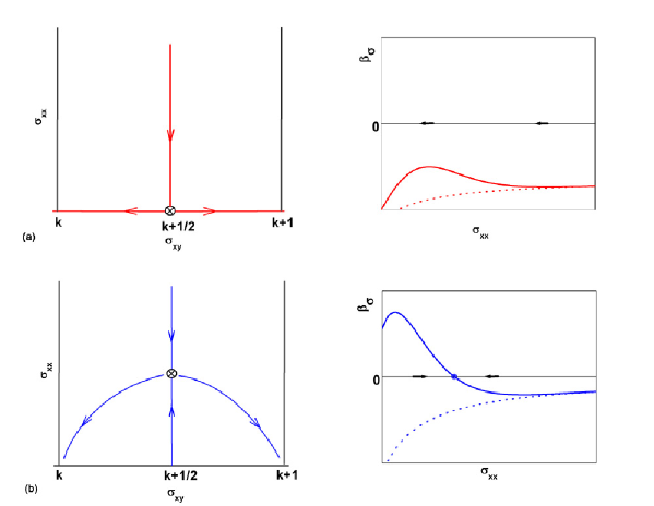
Figure 8: The renormalization group flow diagram for different values of field components $n$ and $m$. (a) The results for large values $n,m\gtrsim 1$. (b) The results for small values $n,m\lesssim 1$.

Equations (262)-(265) are valid in the regime where $L\gg\xi_{M}$ where $\xi_{M}$ denotes the correlation length that describes the cross-over between the weak coupling Goldstone singularities at short distances (described by Eqs (260)) and the quantum Hall singularities (described by Eqs (262)-(265)) that generally occur at much larger distances only. An overall sketch of the renormalization in the $\sigma_{xx}$, $\sigma_{xy}$ conductivity plane is given in Fig. 8a. We see that the infrared of the system is generally controlled by the stable quantum Hall fixed points with $\sigma_{xy}=k(\nu)$ and the unstable fixed points located at $\sigma_{xy}=k(\nu)+1/2$ that describe the singularities of the plateau transitions.

8.2 $0\leq m,n\lesssim 1$

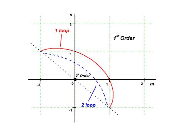
Figure 9: Nature of the transition at $\sigma_{xy}=k+1/2$. The solid red line separates the regions of the first and second order transitions as predicted by $\beta_{\sigma}$, $\beta_{\theta}$, Eqs (260). The dashed blue line is obtained by extending the perturbative contributions to $\beta_{\sigma}$ to include the two-loop results.

Figure 8b illustrates how for small values of $m$ and $n$ the instanton contributions to the $\beta$ functions produce an infrared zero along the line $\theta=\pi$ with $\sigma_{xx}=\mathcal{O}(1)$. This indicates that the transition at $\theta=\pi$ now becomes a true second order one. In Fig.  9 we have plotted the lines in the $m$, $n$ plane that separate the regimes of first order and second order transitions.

To proceed we first address the replica limit $m=n=0$ where the theory describes the physics of the disordered electron gas. The results for the $\beta$ and $\gamma$ functions can be summarized as follows

$$\begin{array}[]{lcccr}\beta_{\sigma}&=&\displaystyle\frac{1}{2\pi^{2}\sigma_{xx}}&+&\displaystyle\frac{16\pi}{e}\sigma_{xx}^{2}e^{-2\pi\sigma_{xx}}\cos 2\pi\sigma_{xy},\\ \beta_{\theta}&=&&&\displaystyle\frac{16\pi}{e}\sigma_{xx}^{2}e^{-2\pi\sigma_{xx}}\sin 2\pi\sigma_{xy},\\ \gamma_{s}&=&-\displaystyle\frac{1}{\pi\sigma_{xx}}&-&\displaystyle\frac{8\pi}{e}\sigma_{xx}e^{-2\pi\sigma_{xx}}\cos 2\pi\sigma_{xy},\\ \gamma_{a}&=&\displaystyle\frac{1}{\pi\sigma_{xx}}&+&\displaystyle\frac{8\pi}{e}\sigma_{xx}e^{-2\pi\sigma_{xx}}\cos 2\pi\sigma_{xy},\\ \gamma_{h}&=&0.&&\end{array}$$ (266)

Here we have extended the quantity $\beta_{\sigma}$ to include the perturbative results obtained to two loop order.

We see that along the lines where $\sigma_{xy}$ is an integer, the instanton contributions generally enhance the tendency of the system toward Anderson localization. Like the theory with large values of $m$ and $n$, this means that the $\beta_{\sigma}$ function renders more positive in the presence of instantons. Unlike the previous case, however, the $\gamma_{h}$ function is now identically zero whereas the $\gamma_{a}$ function becomes manifestly positive. As already mentioned earlier, these results are extremely important and dictated by the physics of the problem.

When $\sigma_{xy}$ is close to half-integer values the perturbative and non-perturbative contributions generally carry the opposite sign. The critical infrared fixed point $\beta_{\sigma}=0$ at $\sigma_{xx}^{*}\approx 0.88$ (Fig.  10) indicates that the electron gas de-localizes. Notice that the situation is in many ways identical to the mobility edge problem in $2+\epsilon$ spatial dimensions except for the fact that the transition is now being approached from the insulating side only.

The consequences of this fixed point for the physics of the electron gas can be summarized as follows.

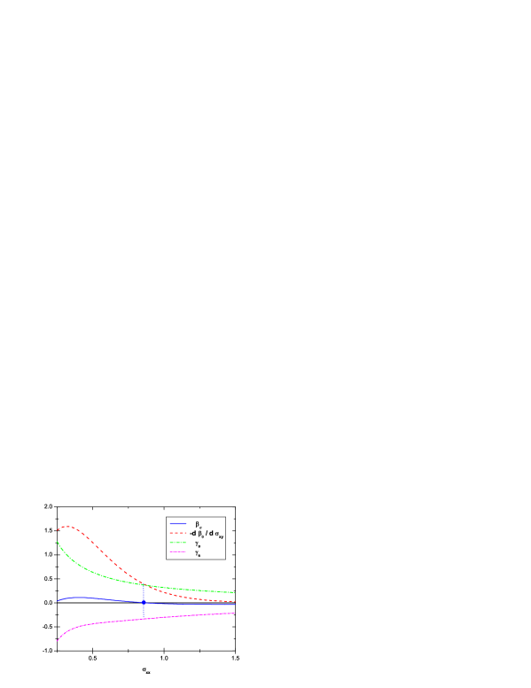
Figure 10: The plot of $\beta_{\sigma}$, $-d\beta_{\theta}/d\sigma_{xy}$, $\gamma_{a}$ and $\gamma_{s}$ as functions of $\sigma_{xx}$ at $\sigma_{xy}=k+1/2$. Blue dot denotes the fixed point.

1. Localization length. Introducing the quantities

$$\Delta_{\theta}=\sigma_{xy}^{0}-k(\nu_{B}^{*})-\frac{1}{2}=\nu_{B}-\nu_{B}^{*},\qquad\Delta_{\sigma}=\sigma_{xx}^{0}-\sigma_{xx}^{*}$$ (267)

which denote the linear environment of the critical fixed point then the divergent localization length $\xi$ of the electron gas can be expressed as

$$\xi=\xi_{0}|\Delta_{\theta}|^{-\nu}.$$ (268)

Here, $\xi_{0}$ is an arbitrary length scale determined by the microscopics of the electron gas and the localization length exponent $\nu$ is obtained as

$$\nu=-\left[\left(\displaystyle\frac{d\beta_{\theta}}{d\sigma_{xy}}\right)^{*}\right]^{-1}\approx 2.8$$ (269)

2. Transport parameters. Next, the ensemble averaged transport parameters of the electron gas can be written as regular functions of two scaling variables $X$ and $Y$ (see Ref. [2])

$$\sigma_{xx}=\sigma_{xx}(X,Y),\qquad\sigma_{xy}=\sigma_{xy}(X,Y),$$ (270)

where

$$X=\left(\frac{L}{\xi_{0}}\right)^{y_{\theta}}\Delta_{\theta},\qquad Y=\left(\frac{L}{\xi_{0}}\right)^{y_{\sigma}}\Delta_{\sigma}$$ (271)

with

$$y_{\theta}=\nu^{-1}\approx 0.36,\qquad y_{\sigma}=-\left(\frac{d\beta_{\sigma}}{d\sigma_{xx}}\right)^{*}\approx-0.17.$$ (272)

Besides the aforementioned results obtained from the large $N$ expansions there exists, until to date, no knowledge on the explicit form of the scaling functions. Nevertheless, there indications which tell us that the functions $\sigma_{xx}(X,Y)$ and $\sigma_{xy}(X,Y)$ are, in fact, very similar for all the cases of interest. For example, recent experiments on quantum criticality in the quantum Hall regime have shown that the scaling functions for the true, interacting electron gas are given by [8]

$$\hskip 71.13188pt\sigma_{xx}(X,Y) = \frac{e^{-X}}{e^{-2X}+1+2Ye^{-X}}$$ (273)

$$\sigma_{xy}(X,Y) = k(\nu)+\frac{1+Ye^{-X}}{e^{-2X}+1+2Ye^{-X}}.$$ (274)

Notice that these results are strikingly similar to those obtained from the large $N$ expansion, in spite of the fact that the two systems in question are physically totally different. Both systems are realizations of an instanton vacuum, however. The results therefore indicate that the list of super universal features of the theory is likely to be extended to include the actual form of the scaling functions $\sigma_{xx}(X,Y)$ and $\sigma_{xy}(X,Y)$.

3. Inverse participation ratio. The electronic wave functions $\Psi_{E}(\textbf{r})$ near the Fermi energy $E$ define a quantity

$$P^{(2)}=\Bigl{\langle}\int d\textbf{r}|\Psi_{E}(\textbf{r})|^{4}\Bigr{\rangle},$$ (275)

which is called the inverse participation ratio. Here, the brackets denote the average with respect to the impurity ensemble. $P^{(2)}$ is a measure for the inverse of the volume that is taken by these electronic levels. It is expected to be zero for extended states and finite for localized states. Hence, this quantity can be used as an alternative probe for Anderson localization. In the language of the non-linear sigma model language we can expressed this quantity in terms of the antisymmetric operator $O_{a}$ according to

$$P^{(2)}\propto\Bigl{\langle}z_{h}O_{a}(Q)\Bigr{\rangle}_{z_{h}\to 0}=\xi^{-D_{2}}f_{2}\left(z_{h}\xi^{d},\Delta_{\sigma}\xi^{y_{\sigma}}\right)|_{z_{h}\to 0}.$$ (276)

Here the expectation is with respect to the non-linear sigma model in the presence of the operator $O_{h}$. The exponent $D_{2}$ equals

$$D_{2}=D-\gamma_{a}^{*}\approx 1.67$$ (277)

with $D=2$ denoting the dimension of the system. It is interesting to remark that the numerical value of $D_{2}$ is largely determined by the perturbative contribution to $\gamma_{a}$, the instanton part merely contributing an amount of roughly three percent.

4. Multifractality. Following Wegner  [30] the generalized inverse participation ratio is defined as follows

$$P^{(q)}=\Bigl{\langle}\int d\textbf{r}|\Psi_{E}(\textbf{r})|^{2q}\Bigr{\rangle}.$$ (278)

The mapping of $P^{(q)}$ onto the non-linear sigma model now involves composite operators with $q$ matrix field variables $Q$. On the basis of this mapping one expects a scaling behavior of the form

$$P^{(q)}\propto\xi^{-(q-1)D_{q}}f_{q}(z_{h}\xi^{d},\Delta_{\sigma}\xi^{y_{\sigma}}).$$ (279)

The generalized dimension $D_{q}$ can be written in terms of the anomalous dimension $\gamma_{q}$ of the composite operators according to

$$D_{q}=D-\frac{\gamma_{q}^{*}}{q-1}.$$ (280)

The following perturbative expression is known  [49]

$$\gamma_{q}=\frac{q(q-1)}{2\pi\sigma_{xx}}+\mathcal{O}(\sigma_{xx}^{-2}).$$ (281)

Based on our results, Eqs (257) and (258), we ready generalize the expression for $\gamma_{q}$ to include the effect of instantons. We obtain

$$\gamma_{q}=\frac{q(q-1)}{2\pi\sigma_{xx}}-\frac{8\pi}{e}\sigma_{xx}B\Bigl{(}\pi\sigma_{xx}q(q-1)\Bigr{)}e^{-2\pi\sigma_{xx}},$$ (282)

where function $B(x)$ is obtained from the $\beta_{0}\to 0$ limit of the ${\tilde{\mathcal{H}}}(\sigma_{xx})$ function and is equal to

$$B(x)=1-\frac{1-e^{-x}}{x}.$$ (283)

The validity of Eq. (282) is likely to be limited to the case of small values of $q$ only, presumably $q\ll 10$. This is so because the higher order terms in the perturbative series for $\gamma_{q}$ are rapidly increasing with increasing values of $q$  [49]. The result for $D_{q}$ becomes

$$D_{q}=D-\frac{q}{2}\gamma^{*}_{a}\left[1-\frac{\gamma^{*}_{a}}{2q(q-1)}B\left(\frac{q(q-1)}{\gamma^{*}_{a}}\right)\right],$$

where $\gamma^{*}_{a}=1/\pi\sigma_{xx}^{*}\approx 0.36$. An important feature of these results is that $\gamma_{q}^{*}\rightarrow 0$ or $D_{q}\rightarrow D$ as $q$ approaches zero. This property permits one to express the multifractal properties of generalized inverse participation ratios in terms of the $f(\alpha)$ singularity spectrum as follows. Introducing the variable

$$\alpha_{q}=D_{q}-(q-1)\frac{dD_{q}}{dq}$$ (284)

then $f(\alpha_{q})$ is given by

$$f(\alpha_{q})=q\alpha_{q}-(q-1)D_{q}.$$ (285)

To proceed let us first consider the perturbative contributions to the generalized dimension $D_{q}$, Eqs (280) and (281). The result can be cast in the familiar form

$$f(\alpha)=D-\frac{(\alpha-\alpha_{0})^{2}}{4(\alpha_{0}-D)},$$ (286)

where

$$\alpha_{0}=D+\frac{1}{2}\gamma_{a}^{*}.$$ (287)

The result of Eq. (286) generally describes the $f(\alpha)$ singularity spectrum near its maximum value at $\alpha=\alpha_{0}$ only. Next, by taking into account the effects from instantons (see Eq. (282)) we find that the expression of Eq. (287) is only slightly modified in that the quantity $\alpha_{0}$ is now given by

$$\alpha_{0}=D+\frac{3}{8}\gamma_{a}^{*}.$$ (288)

Whereas Eq. (287) leads to a numerical value $\alpha_{0}=2.18$, Eq. (288) gives $\alpha_{0}=2.14$. Again we find that the instanton contribution is numerically a small fraction of the final answer. We attribute important significance to these results since they are an integral part of the final conclusion of this paper which says that the quantum critical aspects of the electron gas are within the range of weak coupling expansion techniques.

As a final remark it should be mentioned that the tails of the $f(\alpha)$ singularity spectrum, which are generally controlled by the $D_{q}$ with large values of $q$, is beyond the scope of the present analysis.

8.3 Comparison with numerical work

In Table 2 we compare our results for the critical indices $\nu$, $y_{\sigma}$, $D_{2}$ and $\alpha_{0}$ with those extracted from numerical simulations on the electron gas. The agreement is in many respects spectacular, indicating that our instanton analysis captures some of the most essential and detailed physics of the problem.

Table 2: The critical and multifractal exponents for the model of noninteracting electrons.

Exponent	Instantons	Numerical results
		$2.5\pm 0.5$ [32], $2.34\pm 0.04$ [33]
$\nu$	$2.8\pm 0.4$	$2.3\pm 0.08$ [34], $2.4\pm 0.1$ [35]
		$2.2\pm 0.1$ [36], $2.43\pm 0.18$ [37]
$y_{\sigma}$	$-0.17\pm 0.02$	$-0.38\pm 0.04$ [44], $-0.4\pm 0.1$ [45]
$D_{2}$	$1.67\pm 0.03$	$1.62\pm 0.04$ [38], $1.62\pm 0.02$ [39]
		$1.40\pm 0.02$ [41]
$\alpha_{0}$	$2.14\pm 0.02$	$2.30\pm 0.07$ [42], $2.29\pm 0.02$ [43]
		$2.260\pm 0.003$ [45]

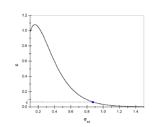
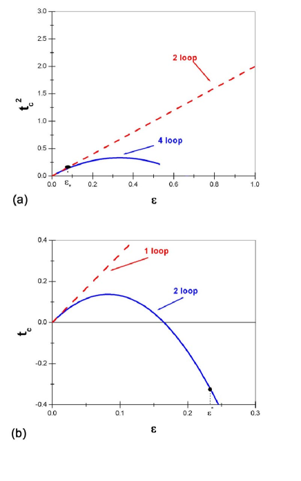
Figure 11: The dependence of $\epsilon$ on the $\sigma_{xx}$ for the model of free electrons $m=n=0$.

Figure 12: The dependence of the critical point $t_{c}=1/\pi\sigma^{*}_{xx}$ from $\epsilon$. (a) The model of free electrons, $m=n=0$. (b) The model with $m=n=0.3$.

The study of the multi fractal aspects of the problem - as done in the previous Section - already indicates that higher order instanton effects are numerically of minor importance. To generally understand why the effects of multi-instanton configurations do not carry much weight, however, one might argue that the very existence of the critical fixed point at $\sigma_{xx}=\sigma_{xx}^{*}$ and $\sigma_{xy}=k(\nu)+1/2$ implies that the corrections due to multi-instantons typically involve factors like $e^{-4\pi\sigma_{xx}^{*}}$ which are negligible as compared to the leading order result $e^{-2\pi\sigma_{xx}^{*}}$. To specify the thought we introduce the quantity

$$\epsilon=\frac{16\pi}{e}\sigma_{xx}e^{-2\pi\sigma_{xx}}.$$ (289)

In the neighborhood of the lines $\sigma_{xy}=k(\nu)+1/2$ the renormalization group functions (266) can then be written in the form of an ordinary $\epsilon$-expansion

$$\hskip 85.35826pt\beta_{\sigma} = -\epsilon\sigma_{xx}+\frac{1}{2\pi^{2}\sigma_{xx}}+\left[\left[\beta_{\sigma}\right]\right],$$ (290)

$$\frac{d\beta_{\theta}}{d\sigma_{xy}} = -2\pi\epsilon\sigma_{xx}+\left[\left[\frac{d\beta_{\theta}}{d\sigma_{xy}}\right]\right],$$

$$\gamma_{s} = \frac{\epsilon}{2}-\frac{1}{\pi\sigma_{xx}}+\left[\left[\gamma_{s}\right]\right],$$

$$\gamma_{a} = -\frac{\epsilon}{2}+\frac{1}{\pi\sigma_{xx}}+\left[\left[\gamma_{a}\right]\right],$$ (291)

$$\gamma_{h} = 0.$$

The brackets $[[\cdots]]$ in the $\beta$ and $\gamma$ functions generally stand for the higher order terms that contain the more complex contributions from the multi-instanton configurations. It is clear, however, that in order for the one-instanton approach to be successful the parameter $\epsilon$ must be a small quantity. By the same token, the expressions $[[\cdots]]$ should be well approximated by inserting the leading order corrections as obtained from ordinary perturbative expansions

$$\hskip 85.35826pt\left[\left[\beta_{\sigma}\right]\right] = \displaystyle\frac{3}{8\pi^{4}\sigma_{xx}^{3}}+\cdots,$$ (292)

$$\left[\left[\displaystyle\frac{d\beta_{\theta}}{d\sigma_{xy}}\right]\right] = 0,$$

$$\left[\left[\gamma_{s}\right]\right] = \displaystyle-\frac{3(1+c)}{8\pi^{3}\sigma_{xx}^{3}}+\cdots,$$

$$\left[\left[\gamma_{a}\right]\right] = \displaystyle\frac{3}{8\pi^{3}\sigma_{xx}^{3}}+\cdots.$$

Here, the constant $c$ has not yet been computed explicitly. The critical fixed point can then be obtained formally as an expansion in powers of $\epsilon$,

$$(\pi\sigma_{xx}^{*})^{-2}=2\epsilon\left(1-\frac{3}{2}\epsilon\right).$$ (293)

Similarly, the critical indices can be obtained as

$$\begin{array}[]{lcrcccr}y_{\theta}&=&\sqrt{2\epsilon}\Bigl{(}1&+&&&\displaystyle\frac{3}{4}\epsilon\Bigr{)},\\ y_{\sigma}&=&-\sqrt{2\epsilon}\Bigl{(}1&-&\displaystyle\frac{3}{2}\sqrt{2\epsilon}&+&\epsilon\Bigr{)},\\ \gamma_{s}^{*}&=&-\sqrt{2\epsilon}\Bigl{(}1&-&\displaystyle\frac{1}{4}\sqrt{2\epsilon}&+&\displaystyle\frac{3c}{4}\epsilon\Bigr{)},\\ \gamma_{a}^{*}&=&\sqrt{2\epsilon}\Bigl{(}1&-&\displaystyle\frac{1}{4}\sqrt{2\epsilon}&&\Bigr{)},\\ \gamma_{h}^{*}&=&0&&&&.\end{array}$$ (294)

A simple computation next tells us that at the fixed point $\sigma_{xx}^{*}$ the parameter $\epsilon$ equals $\epsilon\approx 0.07$ which is indeed a “small” quantity in every respect. In Fig.  12 we have plotted the curve $\epsilon$ with varying values of $\sigma_{xx}$ according to Eq. (289). We see that the fixed point values $\sigma_{xx}^{*}$ and $\epsilon^{*}$ are located well inside the “exponential tail” region where the curve is dominated by the instanton factors $e^{-2\pi\sigma_{xx}}$. In Fig.  12(a) we have plotted the critical value $t^{2}_{c}=(\pi\sigma_{xx}^{*})^{-2}$ with varying values of $\epsilon$ in two-loop approximation where the correction term $\left[\left[\beta_{\sigma}\right]\right]$ in $\beta_{\sigma}$ (see Eqs (290)) has been dropped, as well as in four-loop approximation where this term is retained. The results clearly indicate that the theory with $m=n=0$ lies well inside the regime of validity of the weak coupling expansions as considered in this paper.

Finally, we have used the highest order correction terms in the series of Eq. (294) as an estimate for the uncertainty in the exponent values based on instantons (see Table 2).

8.4 Continuously varying exponents and a conjecture

The critical behavior at $\theta=\pi$ changes continuously as the value of $m$ and $n$ increases. In Figs  13 and 14 we plot our instanton results for the exponents $\nu$ and $y_{\sigma}$ in the interval $0\leq m=n\lesssim 0.3$. In Fig. 15 the results are presented for the three different exponents $\gamma_{i}^{*}$ with varying $m=n$. Of interest is the critical end-point $m=n\approx 0.3$ or, more generally, the boarder line in the $m,n$ plane that separates the regimes of second order and first order phase transitions (Fig. 9). From the mechanism by which the critical fixed point in $\beta_{\sigma}$ is generated (see Fig. 8) it is clear that the boarding line is defined by the points $m,n$ where the exponent $y_{\sigma}$ renders marginal. Along this line the expansion of the $\beta$ functions about the fixed point values $\sigma_{xx}^{*}$ and $\sigma_{xy}^{*}=k(\nu)+1/2$ can be written as follows

$$\hskip 85.35826pt\beta_{\sigma} = -\alpha_{2}\left(\sigma_{xx}-\sigma_{xx}^{*}\right)^{2}$$ (295)

$$\beta_{\theta} = -\nu^{-1}\left(\sigma_{xy}-k(\nu)-\frac{1}{2}\right).$$

Here, $\nu$ equals the correlation length exponent and $\alpha_{2}$ is a positive constant. Notice that the variable $\sigma_{xx}-\sigma_{xx}^{*}>0$ scales to zero in the infrared and, hence, this quantity is marginally irrelevant. On the other hand, the variable $\sigma_{xx}-\sigma_{xx}^{*}<0$ increases with increasing length scales and this quantity is therefore marginally relevant. A characteristic feature of marginally relevant/irrelevant scaling variables is that the critical correlation functions of the system are no longer given by simple power laws but, rather, they acquire logarithmic corrections.

The problem, however, is that the exact location of this line in the $m,n$ plane is beyond the scope of the present analysis. It is easy to see, for example, that the quantity $\epsilon$ (Eq. 289), unlike the theory with $m=n=0$, cannot be considered as a “small” parameter when the values of $m$ and $n$ increase. For illustration we compare in Fig. 12 the critical fixed point $t_{c}=1/\pi\sigma_{xx}^{*}$ with varying values of $\epsilon$ for two different values of $m=n$. Whereas the theory with $m=n=0$ lies well inside the range of validity of the “$\epsilon$ expansion”, this is no longer the case when $m=n\approx 0.3$. At the same time, the expansion is no longer controlled by the exponential tails $e^{-2\pi\sigma_{xx}}$ when the values of $m$ and $n$ increase. All this indicates that the exact location of the critical boarding line in the $m,n$ plane necessarily involves a detailed knowledge of multi-instanton effects.

In spite of these and other complications, however, there are very good reasons to believe that our instanton results display all the qualitative features of quantum criticality in the theory with small $m,n$. It is well known, for example, that the $O(3)$ model at $\theta=\pi$ exhibits a second order phase transition. Since the (algebraic) correlation functions turn out to have logarithmic corrections in this case [50] it is natural to associate the point $m=n=1$ with the aforementioned boarder line in the $m,n$ plane. This means that the regime of second order phase transitions actually spans the interval $0\leq m=n\leq 1$ in Figs 13 - 15, rather than $0\leq m=n\leq 0.3$ as predicted by our instanton analysis. At the same time one expects the global phase diagram (Fig. 9) to be slightly modified and replaced by Fig. 3 in the exact theory.

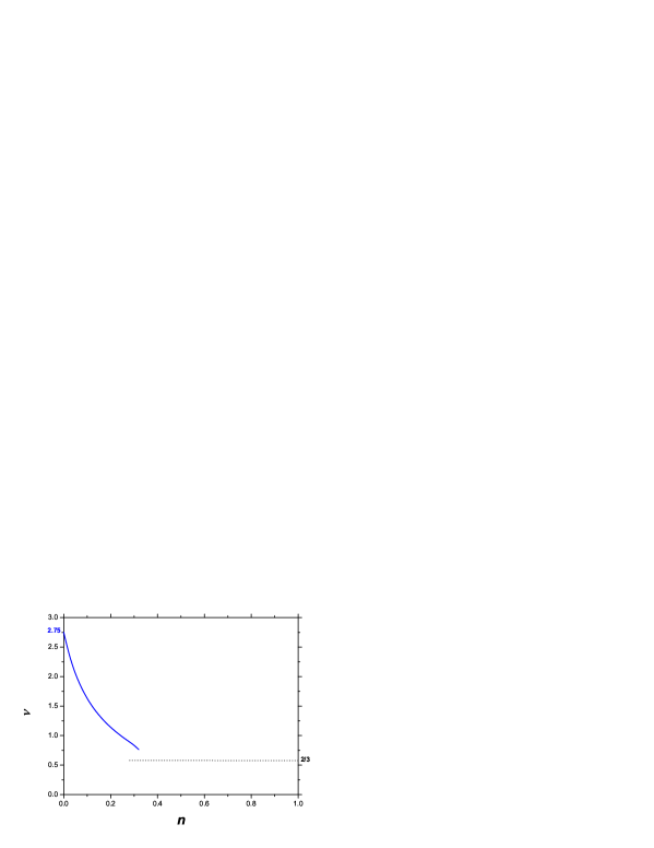
Figure 13: The correlation length exponent $\nu$ with varying values of $0\leq m=n\lesssim 1$. For comparison we have plotted the value $\nu=2/3$ which is known to be the exact result for $m=n=1$, see text.

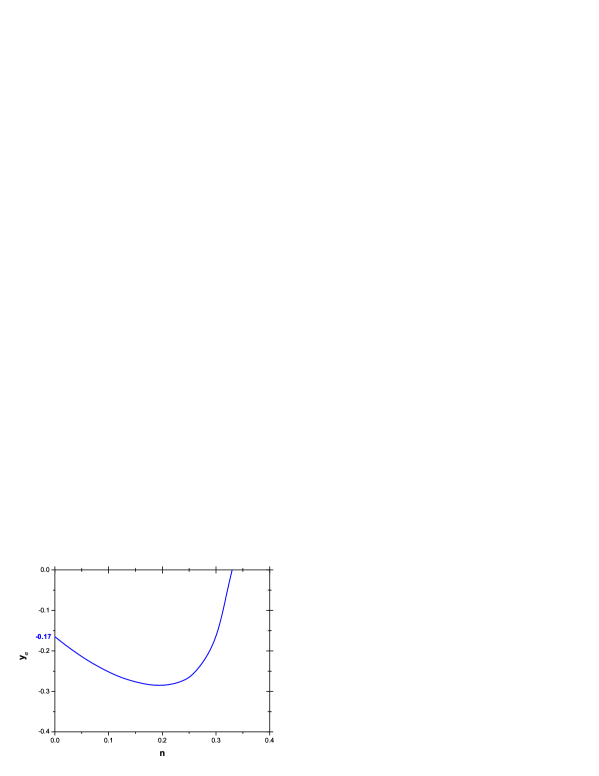
Figure 14: The irrelevant exponent $y_{\sigma}$ with varying values of $0\leq m=n\lesssim 1$, see text.

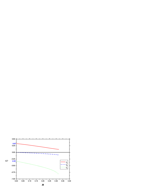
Figure 15: The anomalous dimension $\gamma_{s}^{*}$, $\gamma_{a}^{*}$ and $\gamma_{h}^{*}$ with varying values of $0\leq m=n\lesssim 1$, see text.

9 Conclusion

The results of this paper are an integral part of the general statement which says the physics of the quantum Hall effect is a super universal strong coupling feature of the topological concept of an instanton vacuum in asymptotically free field theory. We have shown that the instanton gas unequivocally describes the cross-over between the Goldstone phase where perturbation theory applies and the completely non-perturbative regime of the quantum Hall effect that generally appears in the limit of much larger distances only.

As a major technical advance we have obtained not only the non-perturbative $\beta$ functions of the theory but also the anomalous dimension or $\gamma$ function associated with mass terms. Amongst many other things, the results of this paper lay the foundation for a non-perturbative analysis of the electron gas that includes the effects of electron-electron interactions.

Whereas the theory with finite $m,n>1$ has been discussed in detail in previous work, on the basis of the large $N$ expansion, the main objective of the present analysis has been the theory with $0\leq m,n\leq 1$. In this case one expects a second order phase transition at $\theta=\pi$ that is characterized by a finite value of $\sigma_{xx}^{*}$ as well as continuously varying exponents. Although much of the global phase structure of the theory was either known or anticipated in previous work by one of us, we have shown that the technical advances made in this paper are nevertheless extremely important. The main difference with the previous situation is that certain ambiguities in the theory have been removed, notably the definition of the $\beta$ functions. Moreover, by extending the theory to include the renormalization group $\gamma$ functions we have not only resolved some of the outstanding problems in the instanton methodology, but also facilitated detailed comparisons between the predictions of the theory on the one hand, and the data known from numerical experiments on the free electron gas on the other.

We have seen that the results of the theory with $m=n=0$ agree remarkably well with the exponent values extracted from numerical simulations (Table 2). Notice that this is the first time - ever since the $\theta$ parameter was introduced in the theory of the quantum Hall effect by one of us - that accurate estimates for the critical indices of the plateau transitions have been obtained analytically. The advances reported in this paper are obviously important since they teach us something fundamental about the strong coupling problems in QCD where the algebra is the same, but experiments are impossible.

10 Acknowlegements

This research was funded in part by the Dutch National Science Foundations NWO and FOM. One of us (IB) is indebted to the Forschungszentrum Jülich (Landau Scholarship), Dynasty Foundation, Russian Foundation for Basic Research (RFBR), and the Russian Ministry of Science for financial support.

Appendix A Appendix. Observable and renormalized theories in $2+\epsilon$ dimensions

Br$\acute{e}$zin et.al. [48] originally showed that the non-linear sigma model in $2+\epsilon$ dimensions generally involves a renormalization of the coupling constant or $\sigma_{xx}$ and one renormalization associated with each of the operators $O_{i}$. Denoting the bare parameters of the theory by $\sigma_{xx}=1/g_{0}$ and $z_{i}^{0}$ then the relation between the bare theory and renormalized theory $g$ and $z_{i}$ is given by

$$\sigma_{xx}=\frac{1}{g_{0}}=\frac{1}{g}\mu^{\epsilon}Z(g),\qquad z_{i}^{0}=z_{i}Z_{i}(g)$$ (296)

with $\mu$ an arbitrary momentum scale. The functions $Z(g)$ and $Z_{i}(g)$ are usually fixed by the requirement that the theory be finite in $\epsilon$. According to the minimum subtraction scheme, for example, one employs the $Z$ and $Z_{i}$ for the purpose of absorbing the pole terms in $\epsilon$ and nothing but the pole terms. However, it is well known that in order to be consistent with the infrared behavior of the theory the terms that are finite in $\epsilon$ can play an important role. Cross-over problems, for example, are treated incorrectly within the minimum subtraction scheme and usually involve a very specific choice of the functions $Z$ that includes terms that are finite in $\epsilon$. In this Section we show that the arbitrariness in the renormalization group is in general avoided if one employs the renormalizations $Z$ and $Z_{i}$ for the purpose of identifying the renormalized and observable theories. For simplicity we shall present the results for the theory in the presence of the operator $O_{h}$ only. It is convenient to introduce a change of variables. Write

$$\sigma_{xx}^{\prime}=\frac{1}{g^{\prime}},\qquad\sigma_{xx}=\frac{1}{g_{0}},$$ (297)

and

$$z_{h}^{\prime}=\frac{(h^{\prime})^{2}}{g^{\prime}},\qquad z^{0}_{h}=\frac{h^{2}_{0}}{g_{0}}.$$ (298)

Since the $g^{\prime},h^{\prime}$ fields have the same meaning for the various Grassmannian manifolds listed in Table 3 we shall from now onward work within the general $G/H$ non-linear sigma model. Starting from the action

$$S=\frac{a}{2}S_{\sigma}[Q]+S_{h}[Q],$$ (299)

Table 3: Coefficients of two-loop computation

$G/H$	$a$	$A_{1}$	$A_{2}$	$B$
$\displaystyle\frac{SO(m+n)}{S(O(m)\times O(n))}$	$1$	$m+n-2$	$2mn-m-n$	$4-2m-2n$
$\displaystyle\frac{SU(m+n)}{S(U(m)\times U(n))}$	$2$	$m+n$	$2(mn+1)$	$0$
$\displaystyle\frac{SP(m+n)}{SP(m)\times SP(n)}$	$4$	$m+n+1$	$\displaystyle 2mn+\frac{m+n}{2}$	$m+n+1$

then a straightforward computation to order $\epsilon^{2}$ of the observable quantities $\sigma_{xx}^{\prime}$ (see Eq. (39)) and $z_{h}^{\prime}$ (see Eq. (45)) yields the following results

$$\frac{1}{g^{\prime}} = \frac{1}{g_{0}}\left(1+A_{1}\frac{g_{0}h^{\epsilon}_{0}}{\epsilon}+\frac{1}{2}\left(A_{2}-B\right)\frac{g^{2}_{0}h^{2\epsilon}_{0}}{\epsilon}-\frac{1}{2}A_{2}Cg^{2}_{0}h^{2\epsilon}_{0}\right),$$ (300)

$$\frac{(h^{\prime})^{2}}{g^{\prime}} = \frac{h^{2}_{0}}{g_{0}}\left(1+\left(A_{1}-\frac{B}{A_{1}}\right)\frac{g_{0}h^{\epsilon}_{0}}{\epsilon}-\left(A_{1}-\frac{B}{A_{1}}\right)\frac{B}{A_{1}}\;\frac{g^{2}_{0}h^{2\epsilon}_{0}}{\epsilon^{2}}\left(1+\frac{\epsilon}{2}\right)\right).$$ (301)

Here, the coefficients $A_{1}$, $A_{2}$ and $B$ are listed in Table 3 and $C$ is a numerical constant. A factor $2\Gamma\left(1-\epsilon/2\right)(4\pi)^{-1-\epsilon/2}$ has been absorbed in a redefinition of the $g_{0}$ and $g^{\prime}$.

The results of Eqs (300) and (301) have originally been used in  [51] for the purpose of expressing the observable parameters in $2+\epsilon$ dimensions in terms of equations of state. Here we shall point out a slightly different interpretation of these results which is obtained by recognizing that the $h^{\prime}$ field actually plays the role of momentum scale that is associated with the observable quantities $g^{\prime}$ or $\sigma_{xx}^{\prime}$ and $z_{h}^{\prime}$. This observation permits one to identify the observable and renormalized theories in the following manner. First we employ Eqs (300) and (301) and eliminate the $h_{0}$ field in the dimensionless combination $g_{0}h_{0}^{\epsilon}$ in favor of the induced momentum scale $h^{\prime}$. The results can be written as

$$\frac{1}{g^{\prime}} = \frac{1}{g_{0}}\left(1+A_{1}\frac{g_{0}(h^{\prime})^{\epsilon}}{\epsilon}+\frac{1}{2}A_{2}\frac{g^{2}_{0}(h^{\prime})^{2\epsilon}}{\epsilon}-\frac{1}{2}A_{2}Cg^{2}_{0}(h^{\prime})^{2\epsilon}\right),$$ (302)

$$\frac{(h^{\prime})^{2}}{g^{\prime}} = \frac{h^{2}_{0}}{g_{0}}\left(1+\left(A_{1}-\frac{B}{A_{1}}\right)\frac{g_{0}(h^{\prime})^{\epsilon}}{\epsilon}-\left(A_{1}-\frac{B}{A_{1}}\right)\frac{B}{A_{1}}\;\frac{g^{2}_{0}(h^{\prime})^{2\epsilon}}{\epsilon^{2}}\right).$$ (303)

As a second step we make use of Eq. (302) and eliminate the bare parameter $g_{0}$ in the combination $g_{0}(h^{\prime})^{\epsilon}$ in favor of the $g^{\prime}$. Introducing the dimensionless quantity

$$\bar{g}=g^{\prime}(h^{\prime})^{\epsilon},$$ (304)

then we obtain from Eqs (302) and (303)

$$\hskip 113.81102pt\frac{1}{g_{0}} = \frac{(h^{\prime})^{\epsilon}}{\bar{g}}Z(\bar{g}),$$ (305)

$$\frac{h^{2}_{0}}{g_{0}} = \frac{(h^{\prime})^{2+\epsilon}}{\bar{g}}\;{Z_{h}(\bar{g})},$$ (306)

where to order ${\bar{g}}^{2}$ the $Z$ and $Z_{h}$ are given by

$$\hskip 85.35826ptZ(\bar{g}) = 1-A_{1}\frac{\bar{g}}{\epsilon}-A_{2}(1-\epsilon C)\frac{\bar{g}^{2}}{2\epsilon},$$ (307)

$${Z_{h}(\bar{g})} = 1-\left(A_{1}-\frac{B}{A_{1}}\right)\frac{\bar{g}}{\epsilon}.$$ (308)

Equations (305) and (306) provide a natural definition of the quantities $Z(g)$ and $Z_{h}(g)$ that appear in the expressions of the renormalized theory, Eqs (296). By fixing the renormalizations $Z$ and $Z_{h}$ according to Eqs (307) and (308) we obtain renormalization group $\beta$ and $\gamma$ functions in the usual manner

$$\beta(g) = \frac{dg}{d\ln\mu}=\frac{\epsilon g}{1-g\displaystyle\frac{d\ln Z}{dg}}=\epsilon g-A_{1}g^{2}-g^{3}A_{2}(1-\epsilon C),$$ (309)

$$\gamma_{h}(g) = -\frac{d\ln z_{h}}{d\ln\mu}=\beta(g)\frac{d}{dg}\ln Z_{h}(g)=-\left(A_{1}-\frac{B}{A_{1}}\right)g+O(g^{3}).$$ (310)

Moreover, the choice of Eqs (305) and (306) implies that the observable theories at different momentum scales $h^{\prime}$ and $h$ respectively can in general be expressed in terms of the $\beta$ and $\gamma$ functions according to

$$\hskip 85.35826pt\bar{g} = g(h^{\prime})=g(h)+\int_{h}^{h^{\prime}}\frac{d\mu}{\mu}\beta(g)$$ (311)

$$z_{h}^{\prime} = z_{h}(h^{\prime})=z_{h}(h)-\int_{h}^{h^{\prime}}\frac{d\mu}{\mu}\gamma_{h}(g)z_{h}(\mu).$$ (312)

The skeptical reader might want to explicitly verify the fact that the results of Eqs (311) and (312) are consistent with the original definition of the observable theory, Eqs (302) and (303). Starting from Eq. (302), for example, one proceeds by inserting ${g_{0}}={h^{-\epsilon}}{g}Z^{-1}(g)$ where $g$ is now defined for momentum scale $h$. This leads to the following expression

$${\bar{g}}=g({h}^{\prime})=g(h)+{\mathcal{I}}\left(g(h),\frac{h^{\prime}}{h}\right)$$ (313)

where

$${\mathcal{I}}\left(g(h),\frac{h^{\prime}}{h}\right) = g\left[\left(\frac{h^{\prime}}{h}\right)^{\epsilon}-1\right]-A_{1}\frac{g^{2}}{\epsilon^{2}}\left\{\epsilon+A_{1}g\left[\left(\frac{h^{\prime}}{h}\right)^{\epsilon}-1\right]\right\}\left(\frac{h^{\prime}}{h}\right)^{\epsilon}$$ (314)

$$\times \left[\left(\frac{h^{\prime}}{h}\right)^{\epsilon}-1\right]-A_{2}\frac{g^{3}}{2\epsilon}\left(1-\epsilon C\right)\left(\frac{h^{\prime}}{h}\right)^{\epsilon}\left[\left(\frac{h^{\prime}}{h}\right)^{2\epsilon}-1\right].$$

Simple algebra next shows that to the appropriate order in $g$ the following identity holds

$$\frac{d}{d\ln{h}}{\mathcal{I}}\left(g(h),\frac{h^{\prime}}{h}\right)=-\beta(g(h)).$$ (315)

This means that Eqs (311) and (313) are indeed identical expressions. Similarly, by starting from Eq. (303), i.e.

$$z_{h}^{\prime}=z_{h}^{0}\left(1+\left(A_{1}-\frac{B}{A_{1}}\right)\frac{g_{0}(h^{\prime})^{\epsilon}}{\epsilon}-\left(A_{1}-\frac{B}{A_{1}}\right)\frac{B}{A_{1}}\;\frac{g^{2}_{0}(h^{\prime})^{2\epsilon}}{\epsilon^{2}}\right),$$ (316)

one obtains the following result for the observable quantity $z_{h}^{\prime}$

$$z_{h}^{\prime}=z_{h}(h^{\prime})=z_{h}(h)+{\mathcal{J}}\left(g(h),\frac{h^{\prime}}{h}\right)$$ (317)

where

$${\mathcal{J}}\left(g(h),\frac{h^{\prime}}{h}\right)=z_{h}(h)\left(A_{1}-\frac{B}{A_{1}}\right)\frac{g}{\epsilon}\left[1-\frac{B}{A_{1}}\frac{g}{\epsilon}\left(\frac{h^{\prime}}{h}\right)^{\epsilon}\right]\left[\left(\frac{h^{\prime}}{h}\right)^{\epsilon}-1\right].$$ (318)

Differentiating with respect to $\ln h$ leads to the following result

$$\frac{d}{d\ln{h}}{\mathcal{J}}\left(g(h),\frac{h^{\prime}}{h}\right)=z_{h}(h)\gamma_{h}(g(h))$$ (319)

which means that Eqs (312) and (317) are identically the same as well.

Appendix B Appendix. Calculation of $\langle S_{h}\rangle$

In order to perform evaluation of $\langle S_{h}\rangle$ for general instanton solution $T_{0}^{-1}R^{-1}\Lambda RT_{0}$ it is convenient to use for matrix $Q$ the parameterization (85). Then we have

$$S_{h}=z_{h}\int\limits_{\eta\theta}\mathop{\rm tr}\nolimits\Lambda_{h}T_{0}^{-1}R^{-1}qRT_{0},$$ (320)

Expanding the matrix $q$ to the second order in $w$ (see Eq.(86)), we obtain

$$S_{h}=S_{h}^{(0)}+S_{h}^{(1)}+S_{h}^{(2)}.$$ (321)

Here the first term

$$S_{h}^{(0)}=z_{h}\int\limits_{\eta\theta}\mathop{\rm tr}\nolimits\Lambda_{h}T_{0}^{-1}R^{-1}\Lambda RT_{0}$$ (322)

is the classical value of $S_{h}$. Next one

$$S_{h}^{(1)}=z_{h}\int\limits_{\eta\theta}\mathop{\rm tr}\nolimits\Lambda_{h}T^{-1}R^{-1}wRT,$$ (323)

contains linear in $w$ terms. The last term in Eq.(320) is as follows

$$S_{h}^{(2)}=-\frac{z_{h}}{2}\int\limits_{\eta\theta}\mathop{\rm tr}\nolimits\Lambda_{h}T^{-1}R^{-1}\Lambda w^{2}RT.$$ (324)

Linear terms. The matrix $(R^{-1}wR)^{\alpha\beta}$ has the following form in the retarded-advanced space for different values of $\alpha$ and $\beta$. If $\alpha=2,\cdots,n$ and $\beta=2,\cdots,m$, then

$$(R^{-1}wR)^{\alpha\beta}=\begin{pmatrix}0&\bar{\Phi}_{0,0}^{(0)}v^{\alpha\beta}\\ \Phi_{0,0}^{(0)}v^{\dagger\alpha\beta}&0\end{pmatrix}.$$ (325)

For $\alpha\neq 1$ we find

$$(R^{-1}wR)^{\alpha 1}=\sqrt{2\pi}\begin{pmatrix}-\bar{\Phi}_{1,0}^{(1)}v^{\alpha 1}&\bar{\Phi}_{1,-1}^{(1)}v^{\alpha 1}\\ \Phi_{1,-1}^{(1)}v^{\dagger\alpha 1}&\Phi_{1,0}^{(1)}v^{{\dagger}\alpha 1}\end{pmatrix}$$ (326)

and analogous for $(R^{-1}wR)^{1\alpha}$. Finally,

$$(R^{-1}wR)^{11}=\sqrt{\frac{4\pi}{3}}\begin{pmatrix}-\frac{1}{\sqrt{2}}\bar{\Phi}_{1,-1}^{(2)}v^{11}-\frac{1}{\sqrt{2}}\Phi_{1,-1}^{(2)}v^{{\dagger}11}&\bar{\Phi}_{1,-2}^{(2)}v^{11}-\Phi_{1,0}^{(2)}v^{{\dagger}11}\\ -\bar{\Phi}_{1,0}^{(2)}v^{11}+\Phi_{1,-2}^{(2)}v^{{\dagger}11}&\frac{1}{\sqrt{2}}\bar{\Phi}_{1,-1}^{(2)}v^{11}+\frac{1}{\sqrt{2}}\Phi_{1,-1}^{(2)}v^{{\dagger}11}\end{pmatrix}.$$ (327)

From Eqs(325)-(327) we see that after integration over $\eta$, $\theta$ the zero modes survive only.

Quadratic terms. The fluctuations $w$ the quadratic term (324) ought to be considered as the massive modes. After averaging over $w$ we obtain

$$\langle S_{h}^{(2)}\rangle=-\frac{z_{h}}{2}\int\limits_{\eta\theta}\mathop{\rm tr}\nolimits\Lambda_{h}T^{-1}R^{-1}\Lambda GRT,$$ (328)

where the matrix $G$ is diagonal in the replica and retarded-advanced spaces

$$G^{\alpha\beta}_{pp^{\prime}}=\delta^{\alpha\beta}_{pp^{\prime}}G^{(\alpha)}_{p}.$$ (329)

The diagonal elements $G^{\alpha}_{p}$ are defined as

$$G^{(\alpha)}_{1}=\begin{cases}\displaystyle\frac{m-1}{O^{(1)}}+\frac{1}{O^{(2)}},&\alpha=1,\\ \displaystyle\frac{m-1}{O^{(0)}}+\frac{1}{O^{(1)}},&\alpha=2,\cdots n.\end{cases}$$ (330)

$$G^{(\alpha)}_{-1}=\begin{cases}\displaystyle\frac{n-1}{O^{(1)}}+\frac{1}{O^{(2)}},&\alpha=1,\\ \displaystyle\frac{n-1}{O^{(0)}}+\frac{1}{O^{(1)}},&\alpha=2,\cdots m.\end{cases}$$ (331)

Hence the matrix $R^{-1}\Lambda GR$ can be written as

$$R^{-1}\Lambda GR=\Lambda G+(R^{-1}\Lambda R-\Lambda)\frac{G_{1}^{(1)}+G^{(1)}_{-1}}{2}.$$ (332)

Thus the renormalization due to the quadratic fluctuations yields

$$\langle S_{h}\rangle=z_{h}\int\limits_{\eta\theta}\left(1-\frac{2}{\sigma_{xx}}\frac{G_{1}^{(1)}+G_{-1}^{(1)}}{2}\right)\mathop{\rm tr}\nolimits\Lambda_{h}T_{0}^{-1}(R^{-1}\Lambda R-\Lambda)T_{0}$$

$$+z_{h}\int\limits_{\eta\theta}\mathop{\rm tr}\nolimits\Lambda_{h}T_{0}^{-1}\Lambda\left(1_{m+n}-\frac{2}{\sigma_{xx}}G\right)T_{0}.$$ (333)

Instanton vacuum. Now we split the matrix $T_{0}\in U(m+n)$ as

$$T_{0}=Wt_{0},\qquad W\in U(m)\times U(n)$$ (334)

and integrate over $W$ in order to restore the $U(m)\times U(n)$ invariance. Then we obtain

$$\langle S_{h}\rangle\to - z_{h}\frac{1}{mn}\int\limits_{\eta\theta}e^{2}_{0}\left(1-\frac{2}{\sigma_{xx}}\frac{G_{1}^{(1)}+G_{-1}^{(1)}}{2}\right)\mathop{\rm tr}\nolimits\Lambda_{h}t_{0}^{-1}\Lambda Xt_{0}$$ (335)

$$+ z_{h}\int\limits_{\eta\theta}\mathop{\rm tr}\nolimits\Lambda_{h}t_{0}^{-1}\Lambda\Bigl{[}1_{m+n}-\frac{1}{mn\sigma_{xx}}$$

$$\times \left(\frac{1}{O^{(2)}}+\frac{m+n-2}{O^{(1)}}+\frac{(m-1)(n-1)}{O^{(0)}}\right)X\Bigr{]}t_{0},$$

where

$$X=(m+n)1_{m+n}+(m-n)\Lambda.$$ (336)

By using the traceless nature of the matrix $\Lambda_{h}$, we find

$$\langle S_{h}\rangle=-z_{h}\frac{m+n}{2mn}\left[1-\frac{1}{4\pi\sigma_{xx}}\int\limits_{\eta\theta}\left(\frac{2}{O^{(2)}}+\frac{m+n-2}{O^{(1)}}\right)\right]\int\limits_{\eta\theta}\mathop{\rm tr}\nolimits\Lambda_{h}t_{0}^{-1}\Lambda t_{0}$$

$$+z_{h}\left[1-\frac{1}{4\pi mn\sigma_{xx}}\int\limits_{\eta\theta}\left(\frac{1}{O^{(2)}}+\frac{m+n-2}{O^{(1)}}+\frac{(m-1)(n-1))}{O^{(0)}}\right)\right]$$

$$\times\int\limits_{\eta\theta}\mathop{\rm tr}\nolimits\Lambda_{h}t_{0}^{-1}\Lambda t_{0}.$$ (337)

Trivial vacuum. The same procedure of taking into account the fluctuations about the trivial vacuum $\Lambda$ instead of Eq.(333) leads eventually to

$$\langle S_{h}\rangle_{0}=z_{h}\int\limits_{\eta\theta}\mathop{\rm tr}\nolimits\Lambda_{h}T_{0}^{-1}\Lambda\left(1_{m+n}-\frac{1}{\sigma_{xx}}\frac{1}{O^{(0)}}X\right)T_{0},$$ (338)

Now it is worth mentioning that due to the traceless nature of the matrix $\Lambda_{h}$ the second part of the matrix $X$ (proportional to $\Lambda$) does not contribute to the $\langle S_{h}\rangle_{0}$. Hence, we obtain

$$\langle S_{h}\rangle_{0}=z_{h}\int\limits_{\eta\theta}\left(1-\frac{m+n}{\sigma_{xx}}\frac{1}{O^{(0)}}\right)\mathop{\rm tr}\nolimits\Lambda_{h}T_{0}^{-1}\Lambda T_{0}.$$ (339)

Finally, we find

$$\langle S_{h}\rangle_{0}=z_{h}\left(1-\frac{m+n}{4\pi\sigma_{xx}}\int\limits_{\eta\theta}\frac{1}{O^{(0)}}\right)\int\limits_{\eta\theta}\mathop{\rm tr}\nolimits\Lambda_{h}T_{0}^{-1}\Lambda T_{0}.$$ (340)

Appendix C Appendix. Matrix elements

Let us define matrix elements of a function $f(\eta,\theta)$ as

$${}_{(a)}\left\langle J,M|f(\eta,\theta)|M^{{}^{\prime}},J^{{}^{\prime}}\right\rangle_{(b)}=\int\limits_{\eta\theta}\Phi_{J,M}^{(a)}(\eta,\theta)f(\eta,\theta)\bar{\Phi}_{J^{{}^{\prime}},M^{{}^{\prime}}}^{(b)}(\eta,\theta),$$

where $a,b=0,1,2$. By using the following relation for the Jacobi polynomials [52]

$$(2n+\alpha+\beta)P_{n}^{(\alpha-1,\beta)}(x)=(n+\alpha+\beta)P_{n}^{(\alpha,\beta)}(x)-(n+\beta)P_{n}^{(\alpha,\beta)}(x),$$ (341)

and the normalization condition

$$\int\limits_{-1}^{1}dx(1-x)^{\alpha}(1+x)^{\beta}P_{n}^{(\alpha,\beta)}(x)P_{m}^{(\alpha,\beta)}(x)\hskip 113.81102pt$$ (342)

$$\hskip 56.9055pt=\delta_{n,m}2^{\alpha+\beta+1}\frac{\Gamma(\alpha+n+1)\Gamma(\beta+n+1)}{(\alpha+\beta+2n+1)\Gamma(n+1)\Gamma(\alpha+\beta+n+1)},$$

we find the following results for diagonal matrix elements of functions $e_{0}^{2}$ and $e_{0}^{4}$

$$\hskip 85.35826pt{}_{(1)}\left\langle J,M|e_{0}^{2}|M,J\right\rangle_{(1)} = \frac{1}{2}\left[1+\frac{2M+1}{4J^{2}-1}\right],$$ (343)

$${}_{(2)}\left\langle J,M|e_{0}^{2}|M,J\right\rangle_{(2)} = \frac{1}{2}\frac{M+1}{J(J+1)},$$

$${}_{(2)}\left\langle J,M|e_{0}^{4}|M,J\right\rangle_{(2)}=\frac{(M+1)(3M-J(J+1)(M-3))-J^{2}(J+1)^{2}}{2J(J+1)(2J-1)(2J+3)}.$$

Performing the summation over $M$ we obtain

$$\hskip 85.35826pt\sum\limits_{M=-J}^{J-1}{}_{(1)}\left\langle J,M|e_{0}^{2}|M,J\right\rangle_{(1)} = \frac{2J}{2},$$

$$\sum\limits_{M=-J-1}^{J-1}{}_{(2)}\left\langle J,M|e_{0}^{2}|M,J\right\rangle_{(2)} = \frac{2J+1}{2}.$$

$$\sum\limits_{M=-J-1}^{J-1}{}_{(2)}\left\langle J,M|e_{0}^{4}|M,J\right\rangle_{(2)} = \frac{2J+1}{3}.$$

Appendix D Appendix. Renormalization around the trivial vacuum with the help of Pauli-Villars procedure

The $\sigma_{xx}$ renormalization. In order to find the renormalization of the $\sigma_{xx}$ conductivity we should compute the average in Eq.(39). Using the parameterization $Q=T_{0}^{-1}qT_{0}$ with the global unitary matrix $T_{0}\in U(m)\times U(n)$ and expanding the $q$ to the second order in $w$, we obtain

$$\sigma_{xx}^{\prime}=\sigma_{xx}+\frac{\sigma_{xx}^{2}}{16mn}\int d\textbf{r}\nabla^{2}\sum\limits_{\alpha,\gamma=1}^{m}\sum\limits_{\beta,\delta=1}^{n}\Bigl{[}\langle v^{\alpha\beta}(\textbf{r})v^{{\dagger}\delta\alpha}(\textbf{r}^{\prime})\rangle_{0}\langle v^{\gamma\delta}(\textbf{r}^{\prime})v^{{\dagger}\beta\gamma}(\textbf{r})\rangle_{0}$$ (344)

$$+\langle v^{\alpha\beta}(\textbf{r})v^{{\dagger}\beta\gamma}(\textbf{r}^{\prime})\rangle_{0}\langle v^{\gamma\delta}(\textbf{r}^{\prime})v^{{\dagger}\delta\alpha}(\textbf{r})\rangle_{0}\Bigr{]},$$

where a point $\textbf{r}^{\prime}$ can be chosen arbitrary since the averages are depend only on the difference of the coordinates. Now by going from $(x,y)$ to $(\eta,\theta)$ coordinates and performing the averages, we find

$$\sigma_{xx}^{\prime}=\sigma_{xx}-2\pi\beta_{0}\int\limits_{\eta\theta}O^{(0)}\mathcal{G}_{0}(\eta\theta;\eta^{\prime}\theta^{\prime})\mathcal{G}_{0}(\eta^{\prime}\theta^{\prime};\eta\theta).$$ (345)

Integrating over $\eta,\theta$ and introducing the Pauli-Villars masses as above, we leads to the following result

$$\sigma_{xx}^{\prime}=\sigma_{xx}-2\pi\beta_{0}\left[\sum\limits_{J=1}\frac{1}{E_{J}^{(0)}}+\sum\limits_{f=1}^{K}\hat{e}_{f}\sum\limits_{J=0}\frac{E_{J}^{(0)}}{(E_{J}^{(0)}+\mathcal{M}^{2}_{f})^{2}}\right]$$ (346)

$$\times\sum\limits_{M=-J}^{J}\Phi_{JM}^{(0)}(\eta^{\prime},\theta^{\prime})\bar{\Phi}_{JM}^{(0)}(\eta^{\prime},\theta^{\prime}).$$

It is worth mentioning that the Jacobi polynomial $P_{J-M}^{M,M}(\eta)$ is proportional to the Gegenbauer polynomial $C_{J-M}^{M+1/2}(\eta)$. By using the summation theorem [52]

$$C_{J}^{\lambda}(\cos\phi\cos\phi^{\prime}+z\sin\phi\sin\phi^{\prime})=\frac{\Gamma(2\lambda-1)}{\Gamma^{2}(\lambda)}\sum\limits_{M=0}^{J}\frac{2^{2M}\Gamma(J-M+1)}{\Gamma(J+M+2\lambda)}\Gamma^{2}(M+\lambda)$$

$$\times(2M+2\lambda-1)\sin^{M}\phi\sin^{M}\phi^{\prime}C^{M+\lambda}_{J-M}(\cos\phi)C^{M+\lambda}_{J-M}(\cos\phi^{\prime})C_{M}^{\lambda-1/2}(z)$$ (347)

with $z=1$ and $\lambda=1/2$, we find that the projection operator

$$\sum\limits_{M=-J}^{J}\Phi_{JM}^{(0)}(\cos\phi,\theta)\bar{\Phi}_{JM}^{(0)}(\cos\phi^{\prime},\theta)=\frac{2J+1}{4\pi}C^{1/2}_{J}\left(\cos(\phi-\phi^{\prime})\right).$$ (348)

Since $C^{1/2}_{J}(1)=1$, we obtain

$$\sigma_{xx}^{\prime}=\sigma_{xx}-\frac{\beta_{0}}{2}\lim\limits_{\Lambda\to\infty}\Biggl{[}\sum\limits_{J=3/2}^{\Lambda}\frac{2J(J^{2}-\frac{1}{4})}{(J^{2}-\frac{1}{4})^{2}}+\sum\limits_{f=1}^{K}\hat{e}_{f}\sum\limits_{J=1/2}^{\Lambda}\frac{2J(J^{2}-\frac{1}{4})}{(J^{2}-\frac{1}{4}+\mathcal{M}^{2}_{f})^{2}}\Biggr{]}.$$ (349)

Finally, evaluation of the sums above yields

$$\sigma_{xx}^{\prime}=\sigma_{xx}-\frac{\beta_{0}}{2}\left(Y^{(0)}_{\rm reg}+1\right)=\sigma_{xx}\left(1-\frac{\beta_{0}}{\sigma_{xx}}\ln\mathcal{M}e^{\gamma}\right)$$ (350)

The $z_{i}$ renormalization. The renormalized quantities $z_{i}^{\prime}$ with $i=a,s,h$ are defined by Eqs (45). Using the parameterization $Q=T_{0}^{-1}qT_{0}$ with the global unitary matrix $T_{0}\in U(m)\times U(n)$ and expanding $q$ to the second order in $w$, we find

$$z_{i}^{\prime}=z_{i}\left(1+\frac{\gamma^{(0)}_{i}\pi}{2mn}\sum\limits_{\alpha=1}^{m}\sum\limits_{\beta=1}^{n}\langle v^{\alpha\beta}v^{{\dagger}\beta\alpha}\rangle_{0}\right).$$ (351)

Here the average $\langle\cdots\rangle_{0}$ is defined with the respect to the action $\delta S_{\sigma}^{(0)}$ (see Eqs  (127)). The averages yield

$$z_{i}^{\prime}=z_{i}\left(1+\frac{2\pi\gamma_{i}^{(0)}}{\sigma_{xx}}\mathcal{G}_{0}(\eta\theta;\eta\theta)\right)$$ (352)

By using Eq.(348), we find

$$z_{i}^{\prime}=z_{i}\left(1+\frac{\gamma_{i}^{(0)}}{2\sigma_{xx}}Y^{(0)}\right).$$ (353)

With a help of the result (153) for the $Y_{\textrm{reg}}^{(0)}$ we finally obtain

$$z_{i}^{\prime}=z_{i}\left(1+\frac{\gamma_{i}^{(0)}}{\sigma_{xx}}\ln\mathcal{M}e^{\gamma-1/2}\right).$$ (354)