Dynamics of Money and Income Distributions

Abstract

We study the model of interacting agents proposed by Chatterjee (2003) that allows agents to both save and exchange wealth. Closed equations for the wealth distribution are developed using a mean field approximation.

We show that when all agents have the same fixed savings propensity, subject to certain well defined approximations defined in the text, these equations yield the conjecture proposed by Chatterjee (2003) for the form of the stationary agent wealth distribution.

If the savings propensity for the equations is chosen according to some random distribution we show further that the wealth distribution for large values of wealth displays a Pareto like power law tail, ie $P(w)\sim w^{1+a}$. However the value of $a$ for the model is exactly 1. Exact numerical simulations for the model illustrate how, as the savings distribution function narrows to zero, the wealth distribution changes from a Pareto form to to an exponential function. Intermediate regions of wealth may be approximately described by a power law with $a>1$. However the value never reaches values of $\sim 1.6-1.7$ that characterise empirical wealth data. This conclusion is not changed if three body agent exchange processes are allowed. We conclude that other mechanisms are required if the model is to agree with empirical wealth data.

url]www.maths.tcd.ie/$\sim$przemek url]www.tcd.ie/Physics/People/Peter.Richmond

1 Introduction

The distribution of wealth or income in society has been of great interest for many years. Italian economist Vilfredo Pareto (1897) was the first to suggest it followed a “natural law” where the higher end of the wealth distribution is described by power law, $P\left(w\right)\sim w^{-1-\alpha}$. Repeated empirical studies Levy Solomon (1997); Dragulescu (2001); Reed Hughes (2002); Aoyama Souma (2003) show that the power law tail exhibits a remarkable spatial and temporal stability and while the value of the exponent, $\alpha$, may vary slightly, it changes little from the value $\sim 1.5$.

Even though the collected data stem from different sources and can be incomplete because of difficulties in accessibility (poor conclusions from income data in Sweden in Levy Solomon (1997) due to a too small number of wealth ranges in the data; total net capital of individual at death in the United States (US) reported to the Bureau of Census and the Inland Revenue for tax heritage purposes in Dragulescu (2001); distributions of sizes of incomes, cities, internet files, biological taxa, gene family and protein family frequencies in Reed Hughes (2002); and income distributions in the Japan in Aoyama Souma (2003)) the common conclusion which can be drawn is that the high end that exhibits the power law is characterised by several multiples or even tens of multiples of the average income/wealth (only $5\%$ of population income-data in the US conforms to a power-law and the power law for the yearly income data in the United Kingdom sets in only for $>50k\pounds$ Dragulescu (2001), income distributions in the Japan in 2000 exhibit power laws only for $>5\cdot 10^{4}$ thousands of Yen).

For around $100$ years the tantalising Pareto law remained without explanation. The renewed interest by physicists and mathematicians in econo- and sociophysics has however led to publication of a number of new papers on the topic in recent years (see Slanina (2004) for an extensive literature review).

The fact that multiplicative power law processes can lead to power law distributions has been known for many years from studies as diverse as the frequency of words in text Yule (1997), economic growth Gibrat (1931), city populations Zipf (1949), wealth distribution Ijiri (1977) and stochastic renewal processes Kesten (1973).

In the analysis of these distributions Solomon (2002) has recently proposed the use of Generalised Lotka Volterra (GLV) equation that combines a multiplicative random process with an autocatalytic process. The latter redistributes a fraction of the total money to ensure the money possessed by an agent is never zero. This simulates in a simplistic way the effect of a tax. The model equations lead to a wealth distribution $P(w)$ of the form:

$$P\left(w\right)\sim\frac{e^{(1-\alpha)/w}}{w^{1+\alpha}}$$ (1)

where and $\alpha-1$ is a positive number that is a ratio of parameters of the model that are related to social security and some random investements respectively. For large values of income $w$ this indeed exhibits a Pareto behaviour.

However two issues arise. The first is that empirical studies of income distributions show that this function does not describe well the very low end of the income distribution which is essentially exponentialDragulescu (2001). The second relates to use of the multiplicative stochastic term. It is certainly necessary to secure the right form for the distribution function but how does it arise in the first place?

More recently Chatterjee (2003) have developed a model of pairwise interacting agents $i$ and $j$ that exchange money by analogy with an ensemble of gas molecules that exchange momentum. In Chatterjee (2003)’s model, however, the agents are allowed to save a fraction $\lambda_{i}$ of their money prior to an interaction. The total money held between two agents is conserved during the interaction process. The governing equations for the evolution of wealth $w_{i}$ and $w_{j}$ of agents $i$ and $j$ respectively are given by:

$$w_{i}\left(t+1\right) = \lambda_{i}w_{i}+\epsilon\left[(1-\lambda_{i})w_{i}+(1-\lambda_{j})w_{j}\right]$$

$$w_{j}\left(t+1\right) = \lambda_{j}w_{j}+\left[1-\epsilon\right]\left[(1-\lambda_{i})w_{i}+(1-\lambda_{j})w_{j}\right]$$ (2)

Here each agent, $i$, has a savings propensity, $\lambda_{i}$. The remaining money is divided during the exchange process in a random manner determined by a uniformly distributed random number $\epsilon$ between zero and one. From their numerical calculations Chatterjee (2003) found the following results for the stationary wealth distribution $P(w)$. Here

1. With no saving ($\lambda_{i}$ = 0 for all $i$) agents behave randomly and the distribution follows the Gibbs rule $P(w)\sim exp(-w/\left<w\right>)$ where $\left<w\right>$ is the average wealth of agent. $P(w)$ has a maximum when $w=0$.

2. If the saving propensity is non-zero and takes the same constant value for all agents ($\lambda_{i}=\lambda$ for all $i$) the resulting distribution can be fitted well by the heuristic function:

   $$P\left(w\right)=\frac{n^{n}}{\Gamma(n)}w^{n-1}\exp\left(-nw\right)$$ (3)

   where $\Gamma(n)$ is the gamma function and the parameter $n$ is related to the saving propensity, $\lambda$ as follows:

   $$n\left(\lambda\right)=1+\frac{3\lambda}{1-\lambda}$$ (4)

   The power, $w^{n-1}$, qualitatively changes the distribution so that it has a maximum for $w>0$. The author does not give any theoretical arguments for the use of this distribution.

3. If the saving propensity for the agents is chosen according to some random distribution, like uniform or power-law distributions with $0\leq\lambda\leq 1$, the numerical output for large values of money gives $P\left(w\right)\sim w^{-1-\alpha}$. This is the celebrated Pareto law. Numerical calculations yield a value for $\alpha=1.03\pm 0.03.$ The authors show empirical data for wealth distributions for both Japan and the USA. These data clearly exhibit power laws with values of $\alpha$ greater than this value. However the authors leave the reader wondering whether the model could fit this data better. A further calculation allowing only a fraction, $p$, of agents to save is made but the the value for the Pareto law remains unchanged. The authors do not investigate the possible changes in $\alpha$ as a result of using savings distributions that differ from uniform distributions.

This work is interesting in that it brings together within one framework the distributions of both Gibbs and Pareto. However it leaves open tantalizing questions.

1. Is it possible to predict analytically the expressions 3 and 4?

2. How does the value of $\alpha$ within the model depend on the nature of the savings distribution?

3. Could it be that the value of $\alpha$ is actually unity?

4. Is there a way of reconciling the approach based on the GLV equations and the exchange theory of Chakrabarti?

Note that caution has to be taken by fitting the models described above to income data obtained from Inland Revenues in different countries. As pointed out in Dragulescu (2000) the wealth has to be understood as a commodity that is subject to an incessant process of exchange rather then as valueables like precious metals, “hard currency”, bonds or works of art that have been deposited in a bank account in order to serve as a lifetime security. In this sense the distributions that come out of the models should be fitted to a momentary distribution of money in the society; a distribution they may or may not be in equillibrium. Since people rarely disclose their momentary wealth the statistical data one avails of regards more the total wealth of individuals, ie the wealth that has been accumulated throughout their whole lifetimes and is reported to the Revenue office only after death (to fulfill the heritage tax requirements). Since, however, individuals with small and medium wealths are rather unlikely to invest parts of their income in any sort of lifetime securities, because their earnings are small and are spent in their total to cover the cost of living, the low end of the momentary money distribution in equillibrium should coincide with the low end of the wealth distribution obtained from the Revenue data. Differences will only be observed in the high end.

In the next section we develop the theory for the model by Chatterjee (2003) and show that it is indeed possible to demonstrate that the conjecture summarised above is, to within a certain well defined approximation, correct. We then study asymptotically the behaviour of the wealth distribution for the case where the savings propensity varies for the agents and demonstrate that if the wealth distribution $P(w)\sim w^{1+\alpha}$ then $\alpha$ is exactly unity for this model. We demonstrate in section 2.2 that this conclusion remains unchanged even when three agent exchange processes are allowed. The conclusions of the mean field analytic analysis are supported by exact numerical simulations shown in Figs. 5 and 6.

2 Theoretical analysis

Complete information about the processes at time t is given by the N agent distribution function $f_{N}(v_{1},\ldots,v_{N}).$ In what follows we shall assume the mean-field approximation. This implies that the $N$-agent distribution function:

$$f_{N}(v_{1},\ldots,v_{N})=P\left(\bigcap_{i}v_{i}\leq V_{i}\leq v_{i}+dv\right)/(dv)^{N}=\prod_{i}f_{1}(v_{i})$$ (5)

We can now invoke the Boltzmann equation Ernst (1981) for the one-agent wealth $v$ distribution $f_{1}(v;t)$ at time $t$. Thus:

$$\partial_{t}f_{1}(v;t)=\int dwdv^{\prime}dw^{\prime}\left(W\left(v\;w|v^{\prime}\;w^{\prime}\right)f_{1}(v^{\prime})f_{1}(w^{\prime})-W\left(v^{\prime}\;w^{\prime}|v\;w\right)f_{1}(v)f_{1}(w)\right)$$ (6)

where the transition probabilities $W\left({}\right)$ are given via the rules for the collision-dynamics (2):

$$W\left(v^{\prime}\;w^{\prime}|v\;w\right)=$$ (7)

$$\delta\left(v^{\prime}-\left(\lambda v+\epsilon(1-\lambda)(v+w)\right)\right)\cdot\delta\left(w^{\prime}-\left(\lambda w+(1-\epsilon)(1-\lambda)(v+w)\right)\right)$$

Introducing the Laplace transform $\tilde{f}_{1}(x;t):=\int_{0}^{\infty}f_{1}(v;t)\exp(-vx)dv$ we obtain an integro-differential equation for the temporal evolution:

$$\partial_{t}\tilde{f}_{1}(x;t)+\tilde{f}_{1}(x;t)=\left\langle\tilde{f}_{2}\left(\lambda x+\epsilon\left(1-\lambda\right)x,\epsilon\left(1-\lambda\right)x;t\right)\right\rangle$$ (8)

where the random spatial variability of the saving propensities $\lambda$ and exchange fractions $\epsilon$ is accounted for by the averaging process $\left\langle{}\right\rangle$ over their random distributions.

We note at this point that this model assumes elastic scattering, i.e. conservation of wealth during the exchange process (2) and the existence of a stationary solution. This is in contrast to many previous models formulated in different contexts where ’wealth’ may be either lost Krapivsky (2002); Ben-Avraham (2003); Bobylev (2000); Baldassarri (2002) or gained Slanina (2004) in the exchange process and the distribution function has a power-law-tail only in an asymptotic sense.

We now write the stationary solutions $\tilde{f}_{1}(x)=lim_{t\longrightarrow\infty}\tilde{f}_{1}(x;t)$ both in terms of solutions of non-linear integral equations (Master Equations (MEs)) and in terms of expansions $\tilde{f}_{1}(x)=\sum_{n=0}^{\infty}(-1)^{n}m_{n}x^{n}$ over moments (Ms) $\left\langle v^{n}\right\rangle=m_{n}\cdot n!$ which satisfy recursion relations. It is convenient to distinguish two cases:

(I) Saving propensity: $\lambda\neq 0$ but equal for all agents:

$$\mbox{ME:}\quad x\tilde{f}_{1}(x)=\frac{1}{1-\lambda}\int_{0}^{(1-\lambda)x}\tilde{f}_{1}(\lambda x+\phi)\tilde{f}_{1}(\phi)d\phi$$ (9)

$$\mbox{Ms:}\quad m_{p}=\sum_{q=0}^{p}m_{q}m_{p-q}\tilde{C}_{q}^{(p)}(\lambda)\quad\mbox{with}\quad\tilde{C}_{q}^{(p)}(\lambda)=\frac{\int_{0}^{(1-\lambda)}\left(\lambda+\eta\right)^{q}\eta^{p-q}d\eta}{1-\lambda}$$ (10)

$$\mbox{and}\quad\tilde{C}_{q+1}^{(p)}=\frac{(1-\lambda)^{p-q-1}-(q+1)\tilde{C}_{q}^{(p)}}{p-q}\quad\mbox{with}\quad\tilde{C}_{0}^{(p)}=\frac{(1-\lambda)^{p}}{p+1}$$ (11)

(II) Random saving propensity: $\lambda\sim\rho_{\Lambda}(\lambda)$.

$$\mbox{ME:}\quad x\tilde{f}_{1}(x)=\int_{0}^{1}d\lambda\frac{\rho_{\Lambda}(\lambda)}{1-\lambda}\int_{0}^{(1-\lambda)x}\tilde{f}_{1}(\lambda x+\phi)\tilde{f}_{1}(\phi)d\phi$$

Here we waive the writing of equations for the moments since due to to the wealth distribution having a power-law tail they may not of course exist. Now an assumption about an asymptotic expansion in the “wealth-domain”: $f_{1}(v)=\sum_{n=0}^{\infty}a_{n}/v^{n+\alpha+1}$ leads to a decomposition of the function in the Laplace domain into two parts

$$\tilde{f}_{1}(x)=\tilde{f}_{1}^{\mbox{reg}}(x)+\tilde{f}_{1}^{\mbox{sing}}(x)$$ (12)

with the first part being an analytic function $\tilde{f}_{1}^{\mbox{reg}}(x)=1-x+O\left(x^{2}\right)$ and the second part $\tilde{f}_{1}^{\mbox{sing}}(x)=\sum_{n=0}^{\infty}b_{n}x^{n+\alpha}$ having a leading term $x^{\alpha}$ of order $\alpha$.

2.1 Conjecture by Patriarca, Chakraborti and Kaski (PCK):

Solving the moments’ equations (10) with initial conditions $m_{0}=1$ and $m_{1}=1$ recursively, ie. expressing, via the $p$th equation, $m_{p}$ as a function of $\lambda$ and all previous values of $m$, (ie $m_{0},m_{1},\ldots,m_{p-1}$), one obtains:

$$m_{2} = \frac{\lambda+2}{2(1+2\lambda)}\quad m_{3}=\frac{\lambda+2}{2(1+2\lambda)^{2}}$$ (13)

$$m_{4} = \frac{72+12\lambda-2\lambda^{2}+9\lambda^{3}-\lambda^{5}}{24(1+2\lambda)^{2}(3+6\lambda-\lambda^{2}+2\lambda^{3})}$$ (14)

The first three moments $m_{1},m_{2}$ and $m_{3}$ coincide with the moments of PCKs function (3) if the relation between the parameters $n$ and $\lambda$ is given by (4). Indeed the coefficients of a series expansion of the Laplace transform

$$\tilde{P}(x)=\int_{0}^{\infty}P(\xi)\exp(-\xi x)d\xi=\left(\frac{n}{x+n}\right)^{n}$$ (15)

of the function (3) agree with moments (14) up to the third order subject to equation (4) being satisfied. This is shown in a nice way in Fig. 1. The deviation $\Delta\tilde{f}_{1}(x)$ between the exact solution of the ME (9) and the ansatz (3) has a leading fourth order:

$$\Delta\tilde{f}_{1}(x)=\frac{(n-1)(n+1)(n+8)}{8n^{3}(10n^{3}+30n^{2}+45n-4)}x^{4}+O\left(x^{5}\right)$$ (16)

It is hard to say if a more general class of functions than (3) would satisfy the ME to higher expansion orders.

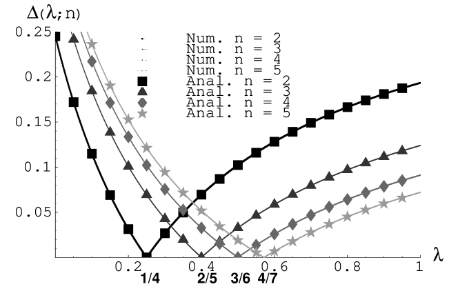
Figure 1: Deviations $\Delta(\lambda;n)=\sum_{p=0}^{10}\left|(m_{p}(\lambda)-m_{p}^{{conj}}(n))/p!\right|$ of the exact moments $m_{p}$ of the wealth distribution from the moments $m_{p}^{{\mbox{conj}}}$ derived from the conjecture plotted as a function of $\lambda$ for $n=2,3\ldots,9$. Solid lines (dot symbols) correspond to analytical (numerical) solutions of the moment equations (10). We see that the minima $\lambda=(n-1)/(n+2)$ $=$ $\left\{1/4,2/5,3/6,4/7,5/8,6/9,7/10,8/11\right\}$ of the deviations do correspond to the PCK conjecture (4).

2.2 The power-law tail:

Calculations by Chatterjee (2003) and ourselves suggest that the value of the exponent $\alpha$ is equal to one. Let us look at this aspect in more detail. Inserting the expansion (12) into the ME (9) and comparing coefficients of order $x^{\alpha+1}$ on both sides of the equation leads to a transcendental equation for the exponent, $\alpha$:

$$\left\langle(1-\lambda)^{\alpha}\right\rangle+\left\langle\frac{1-\lambda^{\alpha+1}}{1-\lambda}\right\rangle=\alpha+1$$ (17)

Clearly if we choose $\alpha=1$, (17) we obtain an indentity for any distribution of $\lambda$. This would seem to be true even for a distribution that assumes only a fraction $p$ of the agents save and the remainder do not save, i.e. $\rho_{\Lambda}^{(1)}(\lambda)=p\rho_{\Lambda}(\lambda)+(1-p)\delta(\lambda)$.

However, whether other solutions for $\alpha$ exist is an open question and depends on the distribution of the saving propensity $\rho_{\Lambda}(\lambda)$. We try to clarify this question below.

For uniformly distributed propensities $\rho_{\Lambda}(\lambda)=1/l_{2}$ for $0\leq\lambda\leq l_{2}\leq 1$ the only solution is $\alpha=1$ (see Fig. 2). Likewise if $\rho_{\Lambda}(\lambda)$ is a normal distribution with a variable mean $l_{2}$ where $\left|l_{2}\right|\leq 1$ and the standard deviation is small (See Fig.3) or with a fixed mean and variable standard deviation (Fig.4) the exponent similarly turns out to be unity.

Now we make a stronger statement and say that there is no continuous and differentiable distribution of saving propensities $\lambda\in[0,1]$ that would yield $\alpha\neq 1$. Indeed since every distribution $\rho_{\Lambda}(\lambda)$ can be constructed as a weighted (possibly continuous) linear combination of uniform distributions

$$\rho_{\Lambda}(\lambda)=\int_{0}^{1}w(\nu)U(0,\nu)d\nu$$ (18)

and since for a uniform distribution $U(0,\nu)$ the left-hand side of the transcendental equation (17) intersects the right-hand side only for $\alpha=1$ in the range $\alpha\in[0,2]$ then the last statement holds also for a generic distribution $\rho_{\Lambda}(\lambda)$. Here we used conditional averaging. This means that the average in equation (17) is carried out as an average over $U(0,\nu)$ conditioned on $\nu$ first and then over the distribution $w(\nu)$ of random values of $\nu$.

Figure 2: The left-hand-side of equation (17) plotted as a function of $\alpha$ for a uniformly random saving propensity $\lambda$ with $0<\lambda<l_{2}$ for different values of $l_{2}$ (dashed lines) and the right-hand-side (rhs) of the equation (17) (solid line). As we can see there is no other solution of the transcendental equation (17) except $\alpha=1$ in the range $\alpha\in[0,2]$.

Figure 3: The same as in Fig.2 but for the propensity $\lambda$ conforming to a truncated $\left|\lambda\right|\leq 1$ normal distribution with variable mean $l_{2}$ and standard deviation $0.01$. As before dashed lines denote the left-hand side and the solid line denotes the right-hand side of equation (17). Again the only solution of the transcendental equation is $\alpha=1$ in the range $\alpha\in[0,2]$.

Figure 4: The same as in Figs.2 and 3 except that now the mean of the normal distribution of propensities $\lambda$ is fixed and equal to $0.5$ and the standard deviation varies. Here again no new solutions except $\alpha=1$ are obtained.

2.3 Beyond the mean-field approximation:

Many-agent distribution functions $f_{N}(x_{1},\ldots,x_{N})$ may not be produced correctly within the mean-field approach. Furthermore the wealth-exchange model by Chatterjee (2003) may be extended to N-point interactions:

$$w_{i}\left(t+1\right)=\lambda_{i}w_{i}+\epsilon_{i}\left[\sum_{j=1}^{N}(1-\lambda_{j})w_{j}\right]\quad\sum_{i}\epsilon_{i}=1$$ (19)

Here we mean that at every time step exchange processes involving any number of agents can happen – each with a certain likelihood. We perform the analysis for $N=3$ in order to find out what kind of mathematical difficulties we will come across. Now the master equation for the 2-agent distribution function in the Laplace domain (compare with (8)) reads:

$$\partial_{t}\tilde{f}_{2}(x,y;t)+\tilde{f}_{2}(x,y;t)=$$ (20)

$$(1-\sigma)\left<\tilde{f}_{2}\left(\lambda x+\lambda_{1}\left(\epsilon x+(1-\epsilon)y\right),\lambda y+\lambda_{1}\left(\epsilon x+(1-\epsilon)y\right);t\right)\right>+$$

$$\frac{\sigma}{2}\left<\tilde{f}_{3}\left(\lambda x+\lambda_{1}\left(\epsilon_{1}x+\epsilon_{2}y\right),\lambda y+\lambda_{1}\left(\epsilon_{1}x+\epsilon_{2}y\right),\lambda_{1}\left(\epsilon_{1}x+\epsilon_{2}y\right);t\right)\right>+$$

$$\frac{\sigma}{2}\left<\tilde{f}_{3}\left(\lambda_{1}\left(\epsilon_{2}x+\epsilon_{3}y\right),\lambda x+\lambda_{1}\left(\epsilon_{2}x+\epsilon_{3}y\right),\lambda y+\lambda_{1}\left(\epsilon_{2}x+\epsilon_{3}y\right);t\right)\right>$$

where $\lambda+\lambda_{1}=1$, $\epsilon+\epsilon_{1}\leq 1$ and $\sigma$ and ($1-\sigma$) denote likelihoods of three-agent and two-agent exchange processes respectively. The first (second and third) term(s) on the right-hand side in (20) account(s) for two-(three-)agent exchange processes repectively. Setting $y=0$ we obtain equation (8) except for three-agent exchange terms that were neglected in the first place and now have been added appropriately. Setting $x=y=0$ we obtain an identity from the normalisation condition $f_{2}(0,0)=f_{3}(0,0,0)=1$.

2.4 The power-law tail with three-agent exchange processes:

Now the transcendental equation, derived from the master equation (20), has the following form:

$$(1-\sigma)\left[\left\langle(1-\lambda)^{\alpha}\right\rangle+\left\langle\frac{1-\lambda^{\alpha+1}}{1-\lambda}\right\rangle\right]+$$ (21)

$$\sigma\frac{2}{\alpha+2}\left[2\left\langle(1-\lambda)^{\alpha}\right\rangle+\left\langle\frac{1-(\alpha+2)\lambda^{\alpha+1}+(\alpha+1)\lambda^{\alpha+2}}{(1-\lambda)^{2}}\right\rangle\right]=\alpha+1$$

and a $\alpha=1$ is again the only solution (compare Fig.5) of this equation for arbitrary saving propensity distributions $\rho_{\Lambda}(\lambda)$ and for any likelihood $\sigma\in[0,1]$ of three-agent exchange processes. This is in conformance with our numerical simulations that also show that an introduction of three-agent exchange processes do not alter the exponent.

Figure 5: The second term (corresponding to three agent exchange processes) on the left-hand-side of equation (21) plotted as a function of $\alpha$ for a uniformly random saving propensity $\lambda$ with $0<\lambda<l_{2}$ for different values of $l_{2}$ (dashed lines) and the right-hand-side (rhs) of the equation (17) (solid line). We see that three-agent exchange processes do not lead to a change of the exponent $\alpha$ from unity to a different value.

2.5 Moment equations in the case of two- and three-agent exchange processes:

The expansion of the steady-state solution in terms of two-agent correlations $\left<v^{p}w^{q}\right>=m_{p,q}\cdot(p!q!)$ now reads $f_{2}(x,y)=\sum_{p,q=0}^{\infty}(-1)^{p+q}m_{p,q}x^{p}y^{q}$ and the two-agent correlations satisfy following equations:

$$m_{p,q}=(1-\sigma)\sum\limits_{{\tiny\begin{array}[]{c}p_{1}+q_{1}=p\\ p_{2}+q_{2}=q\end{array}}}\left(\begin{array}[]{c}p_{1}+p_{2}\\ p_{1}\end{array}\right)\left(\begin{array}[]{c}q_{1}+q_{2}\\ q_{1}\end{array}\right)m_{p_{1}+p_{2},q_{1}+q_{2}}\tilde{C}_{p_{1},q_{2}}^{(p,q)}(\lambda)+$$ (37)

$$\sigma\sum\limits_{{\tiny\begin{array}[]{c}p_{1}+q_{1}+r_{1}=p\\ p_{2}+q_{2}+r_{2}=q\end{array}}}\left(\begin{array}[]{c}p_{1}+p_{2}\\ p_{1}\end{array}\right)\left(\begin{array}[]{c}q_{1}+q_{2}\\ q_{1}\end{array}\right)\left(\begin{array}[]{c}r_{1}+r_{2}\\ r_{1}\end{array}\right)m_{p_{1}+p_{2},q_{1}+q_{2},r_{1}+r_{2}}\tilde{D}_{p_{1},q_{2}}^{(p,q)}(\lambda)$$

where

$$\tilde{C}_{p_{1},q_{1}}^{(p,q)}(\lambda) = \frac{1}{\lambda}\int_{0}^{\lambda_{1}}d\xi\left(\lambda+\xi\right)^{p_{1}}\xi^{p-p_{1}}\left(1-\xi\right)^{q_{1}}\left(\lambda_{1}-\xi\right)^{q-q_{1}}$$

$$\tilde{D}_{p_{1},q_{1}}^{(p,q)}(\lambda) = \frac{2}{\lambda_{1}^{2}}\int_{0}^{\lambda_{1}}d\xi\int_{0}^{\lambda_{1}-\xi}d\eta\left(\lambda+\xi\right)^{p_{1}}\xi^{p-p_{1}}\left(\lambda+\eta\right)^{q_{1}}\eta^{q-q1}$$ (38)

If we neglect ternary exchange processes ($\sigma=0$) we end up with following equations for the moments of the 1-agent distribution function:

$$m_{2}=m_{1,1}\frac{\lambda+2}{2(1+2\lambda)}\quad m_{3}=\frac{m_{1,2}}{1+2\lambda}$$ (39)

$$m_{4}=m_{1,3}\frac{(4-2\lambda+2\lambda^{2}+\lambda^{3})}{2(3+6\lambda-\lambda^{2}+2\lambda^{3})}-m_{2,2}\frac{-6+3\lambda+2\lambda^{2}+\lambda^{3}}{6(3+6\lambda-\lambda^{2}+2\lambda^{3})}$$

$$m_{5}=\frac{((2-2\lambda+3\lambda^{2})m_{1,4}-2(-1+\lambda)m_{2,3})}{(4+8\lambda-3\lambda^{2}+6\lambda^{3})}$$

These equation reduce to equations (14) under the mean-field approximation $m_{p,q}=m_{p}m_{q}$.

3 Exact computer simulations of the model

Intuitively, it is clear that the distribution function depends critically on the relative values of the mean value of the savings propensity and the spread or mean square deviation of the saving distribution function. As the spread of saving propensities tends to zero, the distribution function must change from one having a power law tail to one with an exponential tail. How does this change take place? Could it be that the effective power law region shifts to take on values of $\alpha>1$? Might this explain the empirically observed facts? We have made computer simulations of the model for different values of these parameters. The results are described below.

A uniform distribution of the savings parameter $\lambda$ in the model of Chatterjee (2003) results in a power law distribution of the cumulative distribution shown in the Fig. 6.

The situation is different in the case of $\lambda$ being Gaussian distributed. Here the cumulative wealth distribution may still be approximately described by a power law for widths between 1 and 0.45 (see Fig. 7).

Figure 6: Results of computer simulations, obtained for 500 agents, and 39000 realisations, each taken after 100000 equilibration steps. The data is well described by a power law with exponent -1 in the range of 0.3 up to about 15 times the average money per agent. Changing the width of the distribution of $\lambda$ immediately leads to a loss of the power law. The latter may be a finite size effect since our analytical calculations from section 2.2 show that the power-law does occur for uniform distributions of any widths.

Figure 7: The same as in Fig. 6 but for the saving propensity being Gaussian distributed. Here the power law exponent decreases with decreasing width, but only over a small range from -1 to -1.13. Narrower Gaussian distributions do not result in wealth distributions that can be described by power law. (Note that in the limit of small widths both Gaussian and uniform distribution give the same wealth distribution.)

One thing seems clear. The region where power law behaviour is observed is fairly well marked even when the spread is small. And moreover the slope is consistent with higher values of $\alpha.$ However it does not seem that $\alpha$ can take on values greater than around 1.2. As it stands then we conclude that this model does not offer a complete picture of the empirically observed wealth dynamics.

4 Conclusions

We have studied the model of interacting agents proposed by Chatterjee (2003) that allows agents to both save and exchange wealth. Closed equations for the wealth distribution are developed using a mean field approximation.

We have shown that when all agents have the same fixed savings propensity, subject to certain well defined approximations defined in the text, these equations yield the conjecture proposed by Chatterjee (2003) for the form of the stationary agent wealth distribution.

If the savings propensity for the equations is chosen according to some random distribution we have further shown that the wealth distribution for large values of wealth displays a Pareto like power law tail, ie $P(w)\sim w^{1+a}$. However the value of a for the model is exactly 1. Exact numerical simulations for the model illustrate how, as the savings distribution function narrows to zero, the wealth distribution changes from a Pareto form to to an exponential function. Intermediate regions of wealth may be approximately described by a power law with $a>1$. However the value never reaches values of $\sim 1.6-1.7$ that characterise empirical wealth data. This conclusion is not changed if three body agent exchange processes are allowed. We conclude that other mechanisms are required if the model is to agree with empirical wealth data.

References

- Vilfredo Pareto (1897) Pareto V, Cours d’Economique Politique Lausanne F Rouge 1897
- Slanina (2004) Slanina F, Inelastically scattering particles and wealth distribution in an open economy, Phys. Rev. E 69, n 4, 46102-1-7 (2004)
- Yule (1997) June-Yule Lee, Signal processing of chaotic impacting series, IEE Colloquium on Signals Systems and Chaos, p 7/1-6 (1997)
- Gibrat (1931) Gibrat R, Les Inegalites economiques, Paris, 1931;
- Zipf (1949) Zipf G K, Human Behavior and the Principle of Least Effort, Addison-Wesley 1949
- Ijiri (1977) Ijiri Y and Simon H, Skew Distributions and the Sizes of Business Firms, North-Holland: New York 1977
- Kesten (1973) Kesten H, Random Difference Equations and Renewal Theory for Products of Random Matrices, Acta Mathematica, CXXXI:207-248, 1973
- Solomon (2002) Solomon S et al, Theoretical analysis and simulations of the generalized Lotka-Volterra model, Phys. Rev. E 66, n 3 1, 031102/1-031102/4, (2002); Solomon S, Richmond P, Stable power laws in variable economies; Lotka-Volterra implies Pareto-Zipf, Eur. Phys. J. B 27, n 2, p 257-261, (2002); Richmond P, Solomon S, Power laws are disguised Boltzmann laws Int. J. Mod. Phys. C 12, n 3, p 333-43, (2001)
- Levy Solomon (1997) Levy M, Solomon S, New evidence for the power-law distribution of wealth, Physica A 242, 90, (1997)
- Reed Hughes (2002) Reed W J, Hughes B D, From gene families and genera to incomes and internet file sizes: Why power laws are so common in nature, Phys. Rev. E 66, 067103, (2002)
- Aoyama Souma (2003) Aoyama H, Souma W and Fujiwara Y, Growth and fluctuations of personal and company’s income, Physica A 324, 352, (2003)
- Dragulescu (2001) Dragulescu A and Yakovenko V M, Exponential and power-law probability distributions of wealth and income in the United Kingdom and the United States, Physica A 299, n 1-2, p 213-221, (2001); Dragulescu A, Yakovenko V M, Evidence for the exponential distribution of income in the USA Eur. Phys. J. B 20, n 4, p 585-589 (2001)
- Dragulescu (2000) Dragulescu A and Yakovenko V M, Statistical mechanics of money, Eur. Phys. J. B 17, 723–729 (2000)
- Chatterjee (2003) Chatterjee A and Chakrabarti B K, Money in gas-like markets: Gibbs and Pareto laws, Physica Scripta T 106, p 36-38 (2003) and cond-mat/0311227; Chatterjee A, Chakrabarti B K and Manna S S, Physica A 335 155–163 (2004)
- Ernst (1981) Ernst M H, Nonlinear model-Boltzmann equations and exact solutions, Phys. Rep. (Review Section of Physics Letters) 78, No. 1, p 1-171 (1981)
- Krapivsky (2002) Krapivsky P L and Ben-Naim E, Nontrivial velocity distributions in inelastic gases, J. Phys. A: Math. Gen. 35 L147–L152 (2002)
- Ben-Avraham (2003) Ben-Avraham D, Ben-Naim E, Lindenberg K and Rosas A, Self-similarity in random collision processes Phys. Rev. E, 68, n 5 1, p 50103/1-50103/4 (2003)
- Bobylev (2000) Bobylev A V, Carrillo J A and Gamba I M, On some properties of kinetic and hydrodynamic equations for inelastic interactions J. of Stat. Phys. 98, n 3-4, p 743-73 (2000)
- Baldassarri (2002) Baldassarri A, Puglisi A, Marini U, Marconi B, Kinetics models of inelastic gases, Mathematical Models & Methods in Applied Sciences, 12, n 7, p 965-83 (2002)