Spectral and Diffusive Properties of Silver-Mean Quasicrystals in and Dimensions
Abstract
Spectral properties and anomalous diffusion in the silver-mean (octonacci) quasicrystals in are investigated using numerical simulations of the return probability and the width of the wave packet for various values of the hopping strength . In all dimensions we find , with results suggesting a crossover from to when is varied in , which is compatible with the change of the spectral measure from singular continuous to absolute continuous; and we find with corresponding to anomalous diffusion. Results strongly suggest that is independent of . The scaling of the inverse participation ratio suggests that states remain delocalized even for very small hopping amplitude . A study of the dynamics of initially localized wavepackets in large three-dimensional quasiperiodic structures furthermore reveals that wavepackets composed of eigenstates from an interval around the band edge diffuse faster than those composed of eigenstates from an interval of the band-center states: while the former diffuse anomalously, the latter appear to diffuse slower than any power law.
I Introduction
The discovery of quasicrystalline solid-state structures, characterized by the presence of long-range order but no translational symmetry Shechtman84 , which can be viewed as intermediates between crystalline and amorphous structures Ishimasa85 with icosahedral Shechtman84 , dodecagonal Ishimasa85 , decagonal Bendersky85 , and octagonalWang87 orientational symmetry, as well as the classical wave propagation in quasiperiodic structures Torres03 , renewed the interest in studying quasiperiodic systems, in particular their transport properties Poon92 ; Poon93 ; Roche97 ; Schulz98 ; Mayou00 .
Quantities commonly studied to characterize the electron dynamics in this context are the return probability and the mean-square displacement , defined as
| (1) |
and
| (2) |
where is a wave packet initially located at a site :
| (3) |
One of the characteristic properties of quasiperiodic systems are power-law asymptotic behaviors of these two quantities in the limit , when
| (4) |
and
| (5) |
The exponents satisfy , where the two equalities correspond to the limiting cases of, respectively, the absence of diffusion and the ballistic motion. Inbetween these two cases anomalous diffusion takes place (the classical diffusion is a special case ), leading to the anomalous transport via Einstein’s relation for the zero-frequency conductivity: , where is the diffusion constant, and Eq. (5) leads to the generalized Drude formula , with being a characteristic time beyond which the propagation becomes diffusive due to the scattering Roche97 ; Mayou00 . Furthermore, the shape of the diffusion front of the wavepacket has asymptotically the form of a stretched exponential with in the limit Zhong01 .
The exponent characterizes the spectral properties and equals the correlation dimension of the spectral measure (the local density of states) LDOScorrdim ; Zhong95b . Furthermore, the wavepacket dynamics exhibits multiscaling, where different powers of displacement in Eq. (2) scale with different exponents [Guarneri93, ; Evangelou93, ; Guarneri94, ; Wilkinson94, ; Piechon96, ; Ketzmerick97, ; Barbaroux01, ]. Pure-point, singular continuous and absolute continuous spectra imply, respectively, , and , but the reverse is not necessarily true in general: characterize the continuous spectra, while usually means a pure-point spectrum and the absence of diffusion (), but with nontrivial exceptions Rio95 . One-dimensional quasiperiodic systems commonly have singular continuous spectra Tang86 ; Zhong95b ; Kohmoto87 ; Fujiwara89 ; Sire89 ; Bellissard89 , and may furthermore exhibit transitions from pure-point to absolute continuous behavior (being singular continuous at the transition point) as a parameter in the Hamiltonian is varied, for instance in Harper’s model of an electron in a magnetic field HarpersModel , or the kicked rotator kickedrotator .
Eigenstates of quasiperiodic systems exhibit multifractality, when the electron wavefunction is neither localized nor extended but exhibits self-similarity Tang86 ; Kohmoto87 ; Fujiwara89 ; Niu86 (definitions and further discussion are given in Sec. VI), similar to the Anderson model of localization for disordered conductors near the localization-delocalization transition Schreiber91 .
The Hamiltonian studied in this work (defined in Sec. II) describes a system of atoms of a -dimensional product of th approximants of the silver-mean (octonacci) off-diagonal model.
In a previous work Zhong95b , the direct sum of one-dimensional quasiperiodic systems was studied, and it was shown that already in this case displays non-trivial dimensionally-dependent behavior. On the other hand, it is easy to prove analytically exactly that in quasiperiodic systems defined as a direct sum of one-dimensional quasiperiodic systems, does not depend on the dimensionality of such tilings. In the product systems studied here this is not the case anymore and therefore they can be viewed as a natural next choice for the construction of interesting higher-dimensional quasiperiodic systems in the study of .
The rest of the paper is organized as follows: In Sec. II we define the systems studied, whose eigenproblem is discussed in Sec. III; in Secs. IV and V results of the calculation of and are presented and discussed, respectively; in Sec. VI participation ratios of eigenstates are analyzed, and finally, conclusions are presented in Sec. VII.
II Definitions
The silver-mean chain is defined over an alphabet by the inflation rule
| (6) |
iterated times starting with letter , with the corresponding Hamiltonian
| (7) |
where the sum is restricted to nearest neighbors and the hopping integrals take values and for, respectively, letters and (“large” and “small” hoppings) of the letter sequence of the approximant (with open boundary conditions). Among various number-theoretical properties of the approximants, we mention that the th approximant’s length satisfies , the so-called silver mean.
The -dimensional quasiperiodic tilings we study are derived from the direct product of silver-mean chains Sire89 ; Yuan00 with the Hamiltonian
| (8) |
This has a particularly simple geometrical interpretation, since it describes a particle on a -dimensional cube, with coordinates , hopping only along the main diagonals of the cube: . Since the nearest neighbors of the cube cannot be connected by any number of such hops from , the Hamiltonian (8) decomposes into parts defined on corresponding interpenetrating disconnected quasiperiodic tilings. It can be shown that all of these Hamiltonian parts are equivalent, and that the tilings they define are symmetry related, due to the reflection symmetry of the silver-mean chain about the middle bond of the chain.
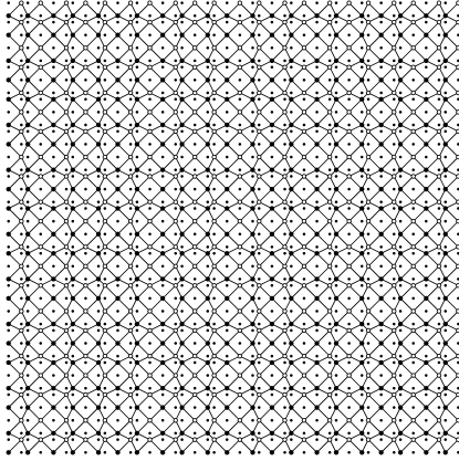
Such tilings in are known as labyrinth tilings, and Figure 1 shows one example, an tiling. The tiling has bipartite structure. Furthermore, a two-dimensional projection of the silver-mean tiling in , for instance, looks exactly as the tiling in Figure 1, because the whole tiling has a layered structure: all symbols of the same kind in the figure belong to one layer. The distance between successive layers are, of course, again determined by the silver-mean sequence. The number of sites in various tilings is given in the Table 1.
III Eigenproblem
The eigenproblem of is
| (9) |
to which the eigenproblem of reduces:
| (11) | |||||
Regarding the subtiling eigenproblem, its eigenstates are obtained simply by projecting the eigenstates of onto the subtiling (with normalization constant ) due to the equivalence of the individual eigenproblems (9). Thus, if denotes the projector onto the subspace of one subtiling, the corresponding subtiling Hamiltonian is and its eigenstates are with the same eigenenergies as in Eq. (11). The reduction of the problem to quasiperiodic subtilings of the product tiling therefore only reduces the degeneracy of individual eigenstates of , while the set of distinct eigenenergies is exactly the same. Furthermore, since all the Hamiltonians studied here have only off-diagonal matrix elements, their eigenenergies necessarily come in opposite-energy pairs, and thus we can restrict our discussion to the spectral properties for states with .
Figure 2 shows the dependence of the eigenenergies on the parameter . A characteristic feature of the spectra is the existence of gaps of various sizes. In , the gap-labeling theorem gives an enumeration of all the possible gaps in the spectrum Kohmoto87 ; gaplabeling . For these gaps seem to close for a sufficiently large , and Fig. 2 suggests that gaps persist only for in , respectively.
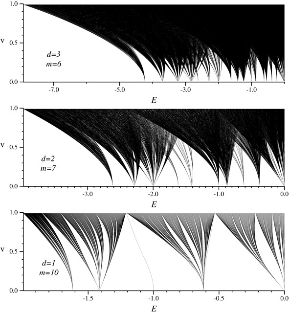
For the gaps close for smaller values of due to the level crossings that are a consequence of the factorizability of the eigenenergies in Eq. (11). Due to this we expect that the spectrum will acquire finite Lebesgue measure and change from from fractal to continuous for intermediate values of , similar to the results of Ref. [Sire89, ].
A more difficult question, that we address in the next section, is whether the spectrum is singular or absolute continuous or a mixture of the two in different regions of the spectrum for various values of . To this end we first note that states corresponding to for are a consequence of the open boundary conditions used in this work, corresponding to the electron localized, for small , at the ends of the chain (in and corners of the cube for ), and spreading across the system as . In this respect the systems studied here are different from those of Ref. [Yuan00, ], where two states have been induced by adding two sites at each end of the chain with . However, for the results presented here this difference in boundary conditions does not play any important role.
IV Return probability and scaling of the spectral measure
In this section we study the scaling of the return probability by evaluating numerically Eq. (1) for the eigenstates of a silver-mean tiling in constructed, as described in the previous section, from eigenstates of the chain, obtained from the numerical diagonalization of the , and taking into account that the time evolution is given by . We present the results in Fig. 3. For small values of there are pronounced steps, and this limit we analyze elsewhere CGS .
For each of the studied cases in the figure, there are three characteristic time-scales of the particle dynamics: (i) short times, characterized by a high probability to find the particle at the initial site, which corresponds to the regime when the wavepacket has only begun spreading; (ii) intermediate times, when does seem to behave according to the power law (4); and (iii) the long-time limit when there is a crossover into a constant , due to the finite spatial extent of the studied systems.

The quantitative determination of is rather difficult, due to the large subdominant contributions to the asymptotic power-law behavior Zhong95b . These appear through the dependence of on the interval of values taken for the least mean-squares linear fit in the log-log plot of . Lacking rigorous results, one attempt to characterize these corrections to Eq. (4) would be to consider a class of power-law subdominant corrections by assuming
| (12) |
It was noted in Ref. [Zhong95b, ] that, in the case of the Fibonacci model, can be accurately fitted to Eq. (12) under the assumption that is exactly equal to , and the authors gave some plausible but non-rigorous arguments for this assumption. On the other hand, numerical verification of Eq. (12) by a least-squares nonlinear fit requires that is calculated for many decades of . In addition, verification of by such a procedure would be particularly difficult near the transition where the fit would be expected to yield already , i.e. to decompose the fitted function into two nearly identical terms. Finally, the parameter would be expected to play some role also in the subdominant terms, for instance through the dependence of the value of on .
An additional difficulty was pointed out in Ref. [Oliviera99, ], where the scaling exponent of the second moment of the spectral measure was considered (which is known LDOScorrdim to be equal to ) for several quasiperiodic systems, including Fibonacci chains, and an apparently irregular behavior of the moment was found in all of the non-Fibonacci models. This led the authors to use a fitting procedure that does not involve fitting of a straight line and even to consider the possibility that the exponent might not exist in these non-Fibonacci systems.
In this work we fit the power law (4) to the calculated values of (for many values of equidistant in the logarithmic scale) by fitting of the expression
| (13) |
in all intervals containing values spanning at least one decade in (for easier comparison, this corresponds to a change in of at least in the plots), and selecting among the obtained fits of those that have values closest to . Should several distinct values of occur that all have small , it seems reasonable that those values corresponding to later times are closer to the correct asymptotic value of , just as it is reasonable to expect that for larger values Eq. (12) becomes close to the power law (4). Our fitting procedure does not assume anything in particular about the subdominant terms of the powerlaw asymptotic behavior, but rather estimates by requiring the absence of certain types of subdominant terms, as quantified by .
We show such obtained fits in Fig. 4 for the case . This is the most difficult system among the three cases presented in Fig. 3 because the duration of the intermediate time regime (ii), where the power law asymptotic behavior should be most likely expected, depends only on the linear size of the system, determined by , and not on the dimensionality . The obtained values of in the fits presented in Fig. 4 range from to .

A characteristic feature of the fits is that for , the time intervals where the power law is obeyed best (i.e. where is smallest) are shorter than the intervals for , even though for large the curves for do not show oscillatory behavior and appear to be more similar to the straight lines. There is, however, a small curvature in the dependence of on for the crossover times inbetween regimes (i) and (ii) as well as (ii) and (iii). This is hard to see in the plots, since it involves large relative changes in small curvatures, but easy to distinguish numerically in our fitting procedure.
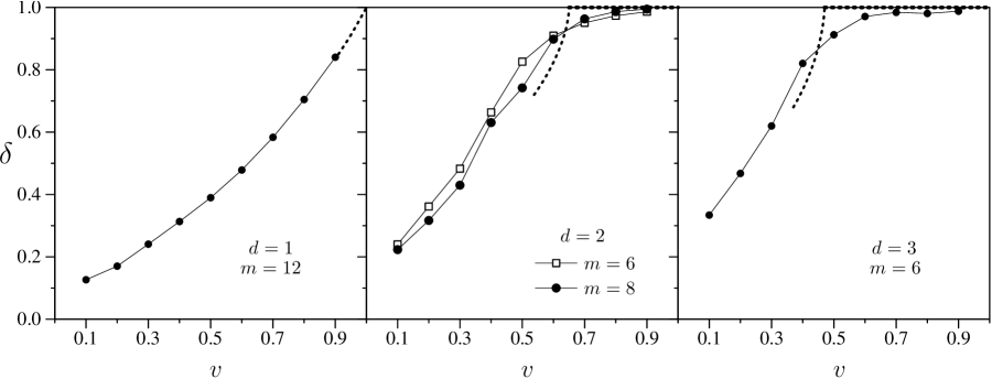
The results for obtained from the above described fitting procedure applied to the results from Fig. 3 are presented in Fig. 5. The plot for shows also for , which is systematically larger than of the system for and smaller for , from which we speculate on the possible form of the limiting curve of the infinite system as indicated in the figure for . This extrapolation of in is in agreement with semi-quantitative considerations of this limit in Ref. [Zhong95b, ]. For the results suggest that for all also in the infinite system. The exponents thus suggest that there is a singular continuous spectrum for all values in and a possible transition from singular continuous to absolute continuous spectra at in (in agreement with a previous estimate Yuan00 ), and at – in .
A difficulty in obtaining exact values of could be due to the possibility that, for , the spectrum is a mixture of singular continuous and absolute continuous parts, when absolute continuous parts appear in only small intervals of the full spectrum that grow larger with increasing , and when the values obtained for away from are closer to the correct asymptotic values.
A previous study Yuan00 of the propagation of the projection of the wave packet (3) onto various segments of the spectrum of the silver-mean model in found that of such restricted wave packets still obeyed the power law, with exponents differing only slightly from obtained when the full spectrum is used. We were able to extend this result by proving the following: If the spectrum is divided into a finite number of segments such that , where is the projector onto the subspace corresponding to the segment , and if in each of the segments, where is defined as in Eq. (1) with the wavepacket (3) replaced by its projection , and if Eq. (4) also holds, then .
V Anomalous diffusion
The main advantage of calculating the width of a wave packet is that it is more directly related to the transport properties than , as discussed in the introduction, and that its asymptotic power-law behavior (5) seems to be less influenced by subdominant contributions, and therefore easier to determine from numerical studies of finite-size systems, as we discuss below.
One of the main difficulties in numerical studies of the anomalous diffusion is that in order to obtain accurately, many eigenvectors are needed. Calculating its behavior at large times also requires large system sizes. This puts significant constraints on the system sizes that can be investigated numerically, and several approximations have been developed to circumvent these difficulties. One of them is to expand the evolution operator in terms of small-time increments Kawarabayashi96 , or to study the time evolution of the position operator expanded in terms of Chebyshev polynomials combined with energy filtering via a Gaussian operator centered at a given energy and of the width of, e.g., of the total bandwidth Triozon03 . In the latter work, generalized quasiperiodic Rauzi tilings have been studied and the authors were interested how the topological connectivity of the tiling influences transport properties of the quasicrystal in . The simplifying feature of the model is that the Hamiltonian is sparse with no matrix elements different from , which significantly speeds up any algorithm where multiplication with the Hamiltonian is a time-consuming part of the calculation, like the algorithm of [Triozon03, ] as well as, for instance, the Lanczos algorithm. Another approach was to study the evolution of a wave packet constructed from a subset of eigenstates from an interval of the full spectrumYuan00 ,
| (14) |
Using such wave packets, the largest system studied in this work is for with 3456000 sites.
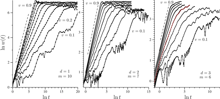
Figure 6 presents results of the calculations of the spreading width of a wave packet initially localized on a single site using all the eigenstates of the spectrum. For small values pronounced steps appear, related to the similar steps in Fig. 3 and the structure of very narrow bands of the spectra (cp. Fig. 2), that we discuss elsewhere CGS .
The three regimes of wave-packet dynamics discussed in the previous section here correspond to (i) the nearly ballistic propagation for early times , (ii) anomalous diffusion, in intermediate intervals of , characterized by Eq. (2) and (iii) a stationary regime of approximately constant , due to the finite extent of the studied systems, for large . The maximum of which would be possible for a system of linear size can be estimated as , corresponding to a state completely localized at the corners of the sample; for the system sizes in Fig. 6, maximal values of are approx. in , respectively. On the other hand, a completely delocalized state would lead to , respectively; thus Fig. 6 shows that for large values of the wave packet becomes smeared out over the entire sample in the regime (iii). The crossover from regime (ii) to (iii) becomes longer for larger , which is due to the more complicated reflection of the wave packet off the boundaries in higher-dimensional tilings.
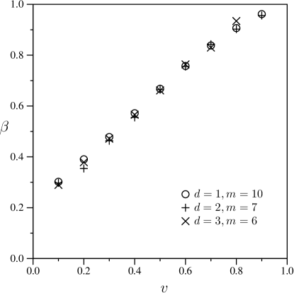
The values of the exponent , which were obtained using the same fitting procedure as in the previous section, are presented in Fig. 7. They seem to be independent of the dimensionality of the system. Since the calculation of is computationally slower than that of , system sizes considered here are smaller than in the previous section, and in particular, for , the power law was observed for only about a half a decade of time for , as opposed to two decades for , and we could not obtain a reliable exponent using our fitting procedure for . In the fitting procedures used in the previous section, for comparison, the calculated exponents were obeyed for at least a decade (and up to 6 decades in some cases for smaller values).
In order to assess the role of topology of the quasiperiodic tiling in , we make a comparison of the wave-packet dynamics studied here with those of Ref. [Triozon03, ]. Since in the latter work energy-filtering was used as described above, we study the spreading of the wave packet (3) composed only of eigenstates with energy in the interval , where is chosen such that the interval contains about of the total number of states.
Figure 8 presents calculated values for several energies between the band edge and the band center. Apparently when the wave packet is composed only of band-edge states, the diffusion is anomalous with the exponent very close to the value obtained when the full spectrum is considered, as indicated in the figure. For other energies, there seems to be an intermediate time regime when anomalous diffusion also takes place, with the same or smaller exponents as compared to the one found at the band edge. Furthermore, a third kind of behavior also occurs, most notably at the band center, where the wave packet seems to spread slower than any power law. This is in qualitative agreement with the findings of [Triozon03, ] in the sense that there wave packets made out of states from the band edge also spread faster but, in contradistinction with the finding here, ballistic motion was found at the band edge and anomalous diffusion at the band center.
It is unclear to us at present what kind of eigenstates are responsible for the slow diffusion seen at the band center. Qualitatively, marginally critical states Fujita01 might be perhaps related to this kind of wavepacket dynamics.

Such constructed wavepackets will inevitably have some “ripples” that depend on how well eigenstates from the chosen interval approximate , which in turn depends on the choice of the starting site . This can be characterized by , and states in Fig. 8 have and at the band edge and the band center, respectively. In order to show some evidence that the obtained dynamics in the two cases does not depend on the choice of the initial site, we present in Fig. 9 when the initial site is chosen two sites along the main diagonal of the system away from the center, in which case and at the band edge and the band center, respectively. The dependence of the values of on the choice of the initial site is reflected in the range of values that takes, but does not seem to affect the two different types of dynamics. Although the contribution of the band edge states to the wave packet in Fig. 9 is much smaller than to that in Fig. 8, the spreading of the entire wave packet is again characterized by the slope in agreement with the value shown in Fig. 7.

VI Participation Ratios
The results of the previous section strongly suggest that is independent of for the class of systems studied here. In this section we attempt to link that with the eigenstate properties by the analysis of the participation number.
The (generalized) inverse participation numbers, , are defined as
| (15) |
The participation number for instance, characterizes on how many sites a given state is significantly different from zero: for a particle completely localized at a single site while for a Bloch wave . The participation ratio, , gives the fraction of the total number of sites where is significantly different from 0.
In the case of the eigenstates of , we have
| (16) | |||||
or, in other words, of the product state is equal to the product of the inverse participation numbers of the one-dimensional states.
On the other hand, the inequality
| (17) |
gives us insight into the nature of eigenstates of : they are always less or equally extended than the most extended state of the product, and more or equally extended than the least extended state of the product. In particular, they can be anisotropically extended, which happens whenever states from the product have quite different participation numbers. For each such state of , there is another one with the same energy and anisotropy in a different direction due to the product structure of the Hamiltonian.
A previous numerical study Yuan00 indicates that the scaling exponents of of the ground state and the band center state are only slightly different. Here, we investigate the scaling of the participation ratio averaged over the whole spectrum as a function of and in , and the results are presented in Fig. 10.

The results indicate that the average participation ratio scales with a power law in the number of sites of the chain,
| (18) |
and the inset of Fig. 10 shows the values of obtained from the least mean-squares linear fit to the data for the largest system sizes in the figure. The results suggest that , which is not surprising since in this limit the quasiperiodic tiling becomes a periodic chain (we note that in our case because we have real instead of complex eigenstates so that the Bloch waves have nodal structure). On the other end, however, , even though for the chain breaks up into clusters of atoms, and therefore . This particular limit we address elsewhere CGS . For we have also calculated numerically for several values and it remains the same within the error bars, which we attribute to the multiplicative nature of the participation numbers as reflected in Eqs. (16) and (17). This can be related to the independence of with respect to the dimensionality determined in the previous section.
VII Conclusions
We studied spectral properties, dynamics of wave packets and scaling properties of eigenstates in 1-, 2- and 3-dimensional systems obtained as direct products of the silver-mean chains, by investigating the scaling exponents and describing the asymptotic properties of, respectively, the return probability, the spreading of the wave packet, and the average participation ratio of eigenstates.
The obtained values of are compatible with the spectral measure being singular continuous in one dimension and undergoing a transition from singular to absolute continuous in with large subdominant contributions. The latter would appear (if such a transition indeed occurs) as a systematic shift of the value of when the system size increases. The comparison of the results for for , and in the two-dimensional systems (cp. Fig. 5) shows such a shift of the order of up to near the speculated transition point and thus corroborates such conclusion. A more quantitative characterization of these corrections, such as, for instance, whether they are of the form (12), is beyond the scope of this work. The obtained values for are independent of the dimensionality, which we have linked to the properties of the inverse participation numbers.
Even though these results are certainly related to the product structure of the quasiperiodic systems studied here, it is quite possible that they describe some features of generic higher-dimensional quasiperiodic systems. In particular, we found an exact relation among the exponent and corresponding exponents of the dynamics of the projection onto subintervals of the spectrum of a wave packet initially localized at a single site, and compared the dynamics of wave packets in the silver-mean quasiperiodic tiling constructed from about of the total number of states near various energies in the band with a study of generalized quasiperiodic Rauzi tilings in Ref. [Triozon03, ]. There seems to be a similarity between the two in so far that wave packets of states near the band edge are spreading much faster than those made out of the states near the band center. However, while in the latter work dynamics of these wave packets is, respectively, ballistic and anomalously diffusive, we find that the dynamics is, respectively, anomalously diffusive and, for the wave packets made out of band-center states, slower than any anomalous diffusion.
Acknowledgements.
One of us (V.Z.C.) gratefully acknowledges discussions with M. Baake and D. Lenz.References
- (1) D. Shechtman, I. Blech, D. Gratias, and J. W. Cahn, Phys. Rev. Lett. 53, 1951 (1984).
- (2) T. Ishimasa, H. U. Nissen, and Y. Fukano, Phys. Rev. Lett. 55, 511 (1985).
- (3) L. Bendersky, Phys. Rev. Lett. 55, 1461 (1985).
- (4) N. Wang, H. Chen, and K. H. Kuo, Phys. Rev. Lett. 59, 1010 (1987).
- (5) M. Torres, J. P. Adrados, J. L. Aragón, P. Cobo, and S. Tehuacanero, Phys. Rev. Lett. 90, 114501 (2003) and references therein.
- (6) S.J. Poon, Adv. Phys. 41, 303 (1992).
- (7) S.J. Poon, F. S. Pierce, Q. Guo, Science 261, 737 (1993).
- (8) S. Roche, G. T. de Laissardiére, and D. Mayou, J. Math. Phys. 38, 1794 (1997).
- (9) H. Schulz-Baldes and J. Bellissard, Rev. Math. Phys. 10, 1 (1998); J. Stat. Phys. 91, 991 (1998).
- (10) D. Mayou, Phys. Rev. Lett. 85, 1290 (2000).
- (11) J. Zhong, R. B. Diener, D. A. Steck, W. H. Oskay, M. G. Raizen, E. Ward Plummer, Z. Zhang, and Q. Niu, Phys. Rev. Lett. 86, 2485 (2001).
- (12) R. Ketzmerick, G. Petschel, and T. Geisel, Phys. Rev. Lett. 69, 695 (1992); M. Holschneider, Commun. Math. Phys. 160, 457 (1994); C. A. Guerin and M. Holschneider, J. Stat. Phys. 86, 707 (1997).
- (13) H. Hiramoto and S. Abe, J. Phys. Soc. Jpn. 57, 230 (1988); 57, 1365 (1988).
- (14) T. Geisel, R. Ketzmerick, and G. Petschel, Phys. Rev. Lett. 66, 1651 (1991).
- (15) C. Tang and M. Kohmoto, Phys. Rev. B 34, 2041 (1986); M. Kohmoto, B. Sutherland, and C. Tang, Phys. Rev. B 35, 1020 (1987); Sütő, A., J. Stat. Phys. 56, 525 (1989); J. Bellissard, B. Iochum, E. Scoppola, D. Testard, Commun. Math. Phys. 125, 527 (1989); D. Damanik and D. Lenz, Commun. Math. Phys. 207, 687 (1999).
- (16) I. Guarneri, Europhys. Lett. 10, 95 (1989); 21, 729 (1993).
- (17) S. N. Evangelou and D. E. Katsanos, J. Phys. A: Math. Gen. 26, L1243 (1993);
- (18) I. Guarneri and G. Mantica, Phys. Rev. Lett. 73, 3379 (1994).
- (19) M. Wilkinson and E. J. Austin, Phys. Rev. B 50, 1420 (1994).
- (20) F. Piéchon, Phys. Rev. Lett. 76, 4372 (1996).
- (21) R. Ketzmerick, K. Kruse, S. Kraut, and T. Geisel, Phys. Rev. Lett. 79, 1959 (1997).
- (22) J-M. Barbaroux , F. Germinet, S. Tcheremchantsev, Duke Math. J. 110, 161-193 (2001).
- (23) R. del Rio, S. Jitomirskaya, Y. Last and B. Simon, Phys. Rev. Lett. 75, 117 (1995).
- (24) J. X. Zhong and R. Mosseri, J. Phys.: Condens. Matter 7, 8383 (1995).
- (25) M. Kohmoto, B. Sutherland, and C. Tang, Phys. Rev. B 35, 1020 (1987).
- (26) T. Fujiwara, M. Kohmoto, and T. Tokihiro, Phys. Rev. B 40, 7413 (1989);
- (27) C. Sire, Europhys. Lett. 10, 483 (1989).
- (28) J. Bellissard, B. Iochum, E. Scoppola, and D. Testard, Commun. Math. Phys. 125, 527 (1989);
- (29) D.R. Hofstadter, Phys. Rev. B 14, 2239 (1976); S. Ostlund, R. Pandit, D. Rand, H. J. Schellnhuber and E. D. Siggia, Phys. Rev. Lett. 50, 1873 (1983); M. Wilkinson, J. Phys. A 20, 4337 (1987).
- (30) F. M. Izrailev, Phys. Rep. 196, 299 (1990); R. Artuso, G. Casati, and D.L. Shepelyansky, Phys. Rev. Lett. 68, 3826 (1992).
- (31) Q. Niu and F. Nori, Phys. Rev. Lett. 57, 2057 (1986).
- (32) M. Schreiber and H. Grussbach, Phys. Rev. Lett. 67, 607 (1991).
- (33) B. Passaro, C. Sire, and V. G. Benza, Phys. Rev. B 46, 13751 (1992).
- (34) J. X. Zhong, J. Bellissard, and R. Mosseri, J. Phys.: Condens. Matter 7, 3507 (1995).
- (35) H. Q. Yuan, U. Grimm, P. Repetowitz, and M. Schreiber, Phys. Rev. B 62, 15569 (2000).
- (36) C. R. de Oliveira and G. Q. Pellegrino, J. Phys. A: Math. Gen. 32, L285 (1999).
- (37) J. Bellissard, A. Bovier, and J. M. Ghez, Rev. Math. Phys. 4, 1 (1992); M. Baake, U. Grimm, and D. Joseph, Int. J. Mod. Phys. B 7, 1527 (1993).
- (38) V. Cerovski, U. Grimm, M. Schreiber, unpublished (2004).
- (39) H. G. E. Hentchel and I. Procaccia, Physica 8D, 435 (1983); T. C. Halsey, M. H. Jensen, L. P. Kadanoff, I. Procaccia, B. I. Shraiman, Phys. Rev. A 33, 1141 (1986).
- (40) T. Kawarabayashi and T. Ohtsuki, Phys. Rev. B 53, 6975 (1996).
- (41) F. Triozon, J. Vidal, R. Mosseri, and D. Mayou, Phys. Rev. B 65, 220202R (2003).
- (42) N. Fujita and K. Niizeki, Phys. Rev. B 64, 144207 (2001).