Duality Relation for Quantum Ratchets

Abstract

A duality relation between the long-time dynamics of a quantum Brownian particle in a tilted ratchet potential and a driven dissipative tight-binding model is reported. It relates a situation of weak dissipation in one model to strong dissipation in the other one, and vice versa. We apply this duality relation to investigate transport and rectification in ratchet potentials: From the linear mobility we infer ground-state delocalization for weak dissipation. We report reversals induced by adiabatic driving and temperature in the ratchet current and its dependence on the potential shape.

Periodic structures with broken spatial symmetry, known as ratchet systems RatRev , present the attractive property of allowing transport under the influence of unbiased forces. The interplay of dissipative tunneling WeiBK99 with unbiased driving enriches the quantum ratchet effect with features absent in its classical counterpart like, e.g., current reversals as a function of temperature ReiPRL97 ; LinSci99 . Quantum ratchet systems have only recently been experimentally realized in semiconductor LinSci99 and superconductor MajPRL03 devices. Also from the theory side there are still few works ReiPRL97 ; SchPRB02 ; LehPRL02 ; RonPRL98 ; GriPRL02 ; MacPRE04 which, with the exception of SchPRB02 ; LehPRL02 , are restricted to the regime of moderate-to-strong damping. After the pioneering semiclassical work ReiPRL97 , further progress towards a quantum description was made in GriPRL02 , where the role of the band structure in ratchet potentials sustaining few bands below the barrier was investigated. Recently, a quantum Smoluchowski treatment MacPRE04 added to the available methods. In this paper, we generalize to an arbitrary ratchet potential a duality relation put forward in Fisher and Zwerger (1985) for a cosine potential. It provides a tight-binding description of quantum Brownian motion in a ratchet potential, and leads to an expression for the ratchet current valid in a wide parameter range including weak dissipation and nonlinear adiabatic driving. We apply this method to discuss rectification and ground-state delocalization occurring for weak dissipation in ratchet potentials. Our results encompass correctly the classical limit.

We consider the Hamiltonian $\hat{H}_{\text{R}}$ of a quantum particle of mass $M$ in a one-dimensional periodic potential $V{(q+L)}=V(q)$ tilted by a time-dependent force $F(t)$,

$$\hat{H}_{\text{R}}(t)=\frac{\hat{p}^{2}}{2M}+V(\hat{q})-F(t)\hat{q}.$$ (1)

The potential assumes in Fourier expansion the form

$$V(\hat{q})=\sum\nolimits_{l=1}^{\infty}{V_{l}\cos{\left(2\pi l\hat{q}/L-\varphi_{l}\right)}},$$ (2)

and can take any shape. Apart from special configurations $\{V_{l}\sin{(\varphi_{l}-l\varphi_{1})}=0\ \forall l\}$ of the amplitudes $V_{l}$ and phases $\varphi_{l}$, this potential is spatially asymmetric and describes a ratchet system. The interaction of the system with a dissipative thermal environment is modeled by the standard Hamiltonian $\hat{H}_{\text{B}}$ of a bath of harmonic oscillators whose coordinates are bilinearly coupled to the system coordinate $\hat{q}$ WeiBK99 . The bath is fully characterized by its spectral density $J(\omega)$. We consider strict Ohmic damping $J(\omega)=\eta\omega$, which reduces to instantaneous viscous damping (viscosity $\eta$) in the classical limit. In such a system, the ratchet effect is characterized by a nonvanishing average stationary particle current $v_{\text{R}}^{\infty}=\lim_{t\to\infty}t^{-1}\int_{0}^{t}dt^{\prime}v(t^{\prime})$ in the presence of unbiased driving, characterized by $\lim_{t\to\infty}t^{-1}\int_{0}^{t}dt^{\prime}F(t^{\prime})=0$, switched on at time $t^{\prime}=0$. In this paper, we shall consider the particular case of unbiased bistable driving switching adiabatically between the values $\pm F$. We report a method to evaluate the stationary velocity $v^{\infty}_{\text{DC}}(F)$ in the biased situation of time-independent driving $F$, which is also of experimental interest MajPRL03 ; LinSci99 . The ratchet current in the presence of adiabatic bistable driving can be expressed as $v_{\text{R}}^{\infty}=v^{\infty}_{\text{DC}}(F)+v^{\infty}_{\text{DC}}(-F)$.

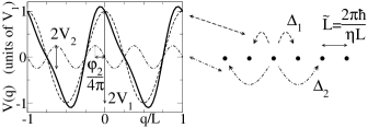
Figure 1: Dual relation between a dissipative ratchet system and a tight-binding (TB) model sketched for a two-harmonics ratchet potential (thick curve). Each harmonic (thin curves) generates couplings to different neighbors in the TB system, according to Eqs. (5) and (7). The periodicity $\tilde{L}$ of the TB model is determined by the viscosity $\eta$ in the original model.

The whole information on the system dynamics is contained in the reduced density matrix $\hat{\rho}(t)=\text{Tr}_{\text{B}}\hat{W}(t)$, obtained from the density matrix $\hat{W}(t)$ of the system-plus-bath $\hat{H}=\hat{H}_{\text{R}}+\hat{H}_{\text{B}}$, with time-independent driving $F$, by performing the trace over the bath degrees of freedom. To evaluate the evolution of the average position $\langle q(t)\rangle=\text{Tr}_{\text{R}}\{\hat{q}\hat{\rho}(t)\}$, the diagonal elements $P(q,t)=\langle q|\hat{\rho}(t)|q\rangle$ of the reduced density matrix are needed, and can be obtained by real-time path integrals techniques WeiBK99 . The velocity follows by time differentiation. At initial time $t^{\prime}=0$, we assume a preparation in a product form where the bath is in thermal equilibrium with the ratchet system $\hat{W}(0)=\hat{\rho}(0)e^{-\beta\hat{H}_{\text{B}}}[\text{Tr}_{\text{B}}e^{-\beta\hat{H}_{\text{B}}}]^{-1}$. The bath temperature is fixed by $T=1/\beta k_{\text{B}}$. This leads to a double path integral

$$P(q_{\text{f}},t)=$$

$$\int dq_{\text{i}}\int dq_{\text{i}^{\prime}}\langle q_{\text{i}}|\hat{\rho}(0)|q_{\text{i}^{\prime}}\rangle\int\limits_{q_{\text{i}}}^{q_{\text{f}}}\mathcal{D}q\int\limits_{q_{\text{i}}^{\prime}}^{q_{\text{f}}}\mathcal{D}^{*}q^{\prime}A[q]A^{*}[q^{\prime}]F[q,q^{\prime}]$$

on the continuous coordinates $q$ and $q^{\prime}$. Here $A[q]=\exp{\{-(it/\hbar)\hat{H}_{\text{R}}\}}$ is the propagator of the ratchet system for a path $q(t^{\prime})$, and $F[q,q^{\prime}]$ the Feynman-Vernon influence functional of the bath inducing nonlocal-in-time Gaussian correlations between the paths $q(t^{\prime})$ and $q^{\prime}(t^{\prime})$ WeiBK99 . Due to the nonlinearity of the potential $V(q)$, these path integrals cannot be performed explicitly. For a cosine potential, Fisher and Zwerger (1985) introduced an exact expansion in the propagator $A[q]$ which transforms the path integrals into Gaussian ones that can be performed. Generalizing this idea for the arbitrary periodic potential (2), we find the expansion

$$\exp\left\{-\frac{i}{\hbar}\int\limits_{0}^{t}dt^{\prime}V\left(q(t^{\prime})\right)\right\}=\sum_{m=0}^{\infty}\sum_{\{l_{j}\}}\prod_{j=1}^{m}\left(\frac{-i\Delta_{l_{j}}}{\hbar}\right)\int\limits_{0}^{t}dt_{m}\int\limits_{0}^{t_{m}}dt_{m-1}\ldots\int\limits_{0}^{t_{2}}dt_{1}\exp\left\{-\frac{i}{\hbar}\int\limits_{0}^{t}dt^{\prime}\rho(t^{\prime})q(t^{\prime})\right\},$$ (4)

where $\rho(t^{\prime})=(2\pi\hbar/L)\sum_{j=1}^{m}l_{j}\delta(t^{\prime}-t_{j})$, and

$$\Delta_{l}=\frac{V_{l}}{2}e^{i\varphi_{l}}\quad\text{for }l>0,\quad\Delta_{-l}=\Delta_{l}^{*}.$$ (5)

The physical meaning of these new quantities will be discussed later. For each term of the sum on $m$ in (4) we have introduced $m$ intermediate times $t_{j}$, and corresponding indices $l_{j}$ taking any value among $\{\pm 1,\pm 2,\ldots\}$. The sum $\sum_{\{l_{j}\}}$ runs on all configurations of these indices. A similar expansion is performed for the propagator $A^{*}[q^{\prime}]$, involving a new set of $m^{\prime}$ times $t_{j}^{\prime}$ and indices $l_{j}^{\prime}$ being used to define $\rho^{\prime}(t^{\prime})$ similarly to $\rho(t^{\prime})$. This enables us to rewrite the average position $\langle q(t)\rangle=\int dqqP(q,t)$ in terms of a series in the amplitudes $V_{l}$ of the potential.

Though still intricate, the resulting expression becomes easier to treat in the long-time limit we are interested in. Quantitatively, the measurement time $t$ should be very long on the time scale $\gamma^{-1}=(\eta/M)^{-1}$ set by dissipation. A second approximation is necessary to proceed: we neglect terms $e^{-\gamma t_{j}}$, $e^{-\gamma t_{j}^{\prime}}$, $e^{-\gamma(t-t_{j})}$, $e^{-\gamma(t-t_{j}^{\prime})}$, $e^{-\omega_{\text{B}}t_{j}}$, $e^{-\omega_{\text{B}}t_{j}^{\prime}}$, $e^{-\omega_{\text{B}}(t-t_{j})}$, and $e^{-\omega_{\text{B}}(t-t_{j}^{\prime})}$, where $\omega_{\text{B}}=2\pi k_{\text{B}}T/\hbar$, in the integrands involved in the series expression for $\langle q(t)\rangle$. We shall refer to this assumption as the rare transitions (RT) limit and discuss its validity later. Generalizing Fisher and Zwerger (1985), we consider a Gaussian wave packet centered at position $q_{0}=\text{Tr}_{\text{R}}[\hat{q}\hat{\rho}(0)]$ and momentum $p_{0}=\text{Tr}_{\text{R}}[\hat{p}\hat{\rho}(0)]$ as initial preparation for the ratchet system. We obtain the important result

$$\langle q(t)\rangle\underset{\genfrac{}{}{0.0pt}{}{t\to\infty}{\text{RT}}}{\sim}q_{0}+\frac{p_{0}}{\eta}+\frac{Ft}{\eta}-\langle q_{\text{TB}}(t)\rangle_{\text{TB}}.$$ (6)

Parts of the series expression for $\langle q(t)\rangle$ has been summed, yielding the first three terms. The rest can be identified with the series expression for the expectation value of the position operator $\hat{q}_{\text{TB}}=\tilde{L}\sum_{n=-\infty}^{\infty}n|n\rangle\langle n|$ of a driven tight-binding (TB) system, described by the Hamiltonian

$$\hat{H}_{\text{TB}}=\sum_{n,l=-\infty}^{\infty}(\Delta_{l}|n+l\rangle\langle n|+\Delta_{l}^{*}|n\rangle\langle n+l|)-F\hat{q}_{\text{TB}},$$ (7)

and bilinearly coupled to a different bath of harmonic oscillators. The spectral density of this bath $J_{\text{TB}}(\omega)=J(\omega)/[1+\left(\omega/\gamma\right)^{2}]$ is still Ohmic but presents a cutoff at the frequency $\gamma$ set by dissipation. At initial time $t^{\prime}=0$ the TB system is prepared in the state $|n=0\rangle$. The calculation shows that the $\Delta_{l}$ introduced in (5) are identified with the couplings of the TB system (7). We stress that the $l\text{th}$ harmonic of the original potential results in a coupling to the $l\text{th}$ neighbors in the dual TB system as sketched in Fig. 1. One can easily show that the spatial symmetry condition on the phases $\varphi_{l}$ is the same in both systems. The first three terms on the right-hand side of (6) reproduce exactly the classical solution for the average position $\langle q(t)\rangle$ of a free system, $V(q)\equiv 0$, at long times. In this linear case, the quantum and classical solutions should be identical, due to Ehrenfest theorem, and they are, because the TB average $\langle q_{\text{TB}}(t)\rangle_{\text{TB}}$ vanishes in the absence of the potential $V(q)$. We expect the same result when the potential is present but unimportant, e.g., for large driving $F$ and/or high temperatures $T$.

The series expression for the diagonal elements of the reduced density matrix $\hat{\rho}_{\text{TB}}$ of the TB system, which leads to the series expression for $\langle q_{\text{TB}}(t)\rangle_{\text{TB}}$, can be written in terms of pairs of TB trajectories $q_{\text{TB}}(t^{\prime})=\eta^{-1}\int_{0}^{t^{\prime}}dt^{\prime\prime}\rho(t^{\prime\prime})$ [with $\rho(t^{\prime})$ introduced above Eq. (5)], and $q^{\prime}_{\text{TB}}(t^{\prime})$ defined similarly in terms of $\rho^{\prime}(t^{\prime})$. From that one extracts the spatial periodicity $\tilde{L}$ of the TB system, yielding $\tilde{L}=L/\alpha$, where $\alpha=\eta L^{2}/2\pi\hbar$ is the dimensionless dissipation parameter of the original system. These pairs of trajectories combine in discrete paths in the $q-q^{\prime}$ plane parametrized by pairs of integers $(n,n^{\prime})$.

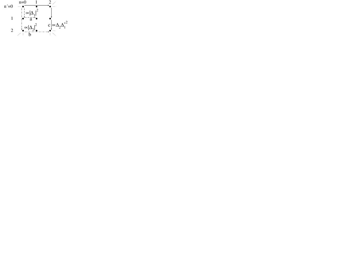
Figure 2: Representation of some of the second-order (a,b) and third-order (c) paths contributing to the diagonal elements of the reduced density matrix of the tight-binding model, and the corresponding dependence on the couplings $\Delta_{l}$.

Each path starting in the diagonal element $(0,0)$ and ending at time $t$ in $(m,m)$ contributes to $\langle m|\hat{\rho}_{\text{TB}}(t)|m\rangle$. Each transition in the path brings a corresponding factor $\Delta_{l}$ and all paths involve at least two transitions (cf. Fig. 2). Written in this form, the diagonal elements of the reduced density matrix are a solution of a generalized master equation GriPRE96 in terms of transition rates $\Gamma_{m}$ from the TB site $(n,n)$ to the site $(n+m,n+m)$. Consequently, these rates are expressed in power series of all the couplings $\Delta_{l}$, starting from second order. As the times $t_{j},t^{\prime}_{j}$ introduced in (4) are identified with the transition times in the TB representation, the rates $\Gamma_{m}$ give also a way to control our assumption of rare transitions. It corresponds to neglect those paths which involve transitions on a time scale $\max(\gamma^{-1},\omega_{\text{B}}^{-1})$ after the initial time $t^{\prime}=0$ or before the final time $t^{\prime}=t$. As transitions in the TB model happen on a time scale $\Gamma_{m}^{-1}$, the duality relation will be valid when the transitions are rare on the time scale $\max(\gamma^{-1},\omega_{\text{B}}^{-1})$, i.e., when all rates satisfy $\Gamma_{m}\ll\min(\gamma,\omega_{\text{B}})$. This condition is controlled by the dissipation through $\gamma=\eta/M$ and the temperature through $\omega_{\text{B}}=2\pi k_{\text{B}}T/\hbar$.

Due to the change of periodicity length between the two systems, the dissipation parameter $\alpha$ and the energy drop per unit cell $\epsilon=FL$ become $\tilde{\alpha}=1/\alpha$ and $\tilde{\epsilon}=\epsilon/{\alpha}$ in the TB system. Thus, weak dissipation in one system maps to strong dissipation in the other one although the viscosity $\eta$ in the spectral density does not change. The asymptotic dynamics is usually described by the nonlinear mobility $\mu=\lim_{t\to\infty}v(t)/F$. With these notations, the duality relation (6) can be rewritten in the form

$$\mu(\alpha,\epsilon)\xrightarrow[\text{RT}]{}\mu_{0}-\mu_{\text{TB}}(1/\alpha,\epsilon/\alpha),$$ (8)

where $\mu_{0}=1/\eta$ is the mobility of the free system, $V(q)\equiv 0$. In the special case of a cosine potential, this relation was already obtained in Fisher and Zwerger (1985) for the dc mobility. It it also interesting to notice that it was also derived in SasPRB96 for the linear ac mobility in a cosine potential. However, we did not completely succeed in generalizing Eq. (8) in the presence of time-dependent driving.

We shall now focus on the evaluation of the stationary velocity $v^{\infty}_{\text{DC}}(F)$. By solving the generalized master equation mentioned above, one finds the stationary velocity $v^{\infty}_{\text{TB}}=\tilde{L}\sum_{m}m\Gamma_{m}$ in the dissipative TB system. The duality relation (6) can then be used to obtain

$$v^{\infty}_{\text{DC}}(F)=F/\eta-(L/\alpha)\sum\nolimits_{m=1}^{\infty}m(\Gamma_{m}-\Gamma_{-m}).$$ (9)

As discussed above, the rates $\Gamma_{m}$ are power series in the couplings $\Delta_{l}$ starting from second order. For a given $m\neq 0$, there are only two possible second-order contributions to $\Gamma_{m}$, which, after use of Eq. (5), sum up to WeiBK99

$$\Gamma_{m}^{(2)}=\frac{V_{m}^{2}}{4\hbar^{2}\gamma}\int\nolimits_{-\infty}^{\infty}d\tau\ e^{-m^{2}\tilde{\alpha}Q(\tau)+im(F\tilde{L}/\hbar\gamma)\tau}.$$ (10)

The influence of the dissipative environment enters through the dimensionless bath correlation function $Q(\tau)=2\int_{0}^{\infty}\frac{d\omega}{\omega(1+\omega^{2})}\left[\coth{(\omega/2\theta)}(1-\cos{\omega\tau)}+i\sin{\omega\tau}\right]$ with $\theta=k_{\text{B}}T/\hbar\gamma$. At zero bias $F=0$ and in the scaling limit $\hbar\gamma\gg k_{\text{B}}T$, the rates show a power-law dependence on temperature $\Gamma_{m}^{(2)}\propto T^{2m^{2}\tilde{\alpha}-1}$. The linear mobility $\mu_{\text{TB}}$ is thus dominated by the rate $\Gamma_{1}^{(2)}$ at low temperatures, and vanishes at $T=0$ for $\alpha<1$, which corresponds to free dynamics $\mu=\mu_{0}$ in the dual weak-binding system note0 . This suggests that the occurrence of a delocalization to localization transition at $\alpha=1$ for the ground state of a cosine potential Fisher and Zwerger (1985); SchPRL83 would not be affected in more general potentials (see also Fig. 3).

In the remainder of the paper, we focus on the ratchet current induced by adiabatic bistable driving $v_{\text{R}}^{\infty}=v^{\infty}_{\text{DC}}(F)+v^{\infty}_{\text{DC}}(-F)$. The second-order rates obey $\Gamma_{m}^{(2)}(-F)=\Gamma_{-m}^{(2)}(F)$ and therefore cancel out in the expression for the ratchet current. Hence, we have to focus on contributions of at least third order to the rates $\Gamma_{m}$. Here we neglect higher orders. This is known to provide a good approximation in TB systems with large dissipation parameter $\tilde{\alpha}$ and/or high temperature WeiBK99 . For simplicity we also consider a potential consisting of only two harmonics. There is no problem of principle to include more harmonics note1 . We find, with $m=\pm 1,\pm 2$,

$$\Gamma_{m}^{(3)}=\frac{V_{1}^{2}V_{2}}{4\hbar^{3}\gamma^{2}}\operatorname{Im}\left[\int\nolimits_{-\infty}^{\infty}d\tau\ G_{|m|}^{(3)}(\tau)\ e^{im(F\tilde{L}/\hbar\gamma)\tau-i\operatorname{sgn}(m)\varphi}\right],$$ (11)

where we have introduced $\varphi=\varphi_{2}-2\varphi_{1}$, and

$$G_{1}^{(3)}(\tau)=-\int\nolimits_{0}^{\infty}d\rho\ e^{-2\tilde{\alpha}Q(\rho)}$$

$$\times\left[e^{-2\tilde{\alpha}Q(\tau+\rho)+\tilde{\alpha}Q(\tau+2\rho)}+e^{-2\tilde{\alpha}Q(\tau-\rho)+\tilde{\alpha}Q(\tau-2\rho)}\right],$$

$$G_{2}^{(3)}(\tau)=\int\nolimits_{0}^{\infty}d\rho\ e^{\tilde{\alpha}Q(\rho)-2\tilde{\alpha}Q(\tau+\rho/2)-2\tilde{\alpha}Q(\tau-\rho/2)}.$$ (12)

At third order the rates obey $\Gamma_{m}^{(3)}(F,\varphi)=\Gamma_{-m}^{(3)}(-F,-\varphi)$, which is a consequence of parity. The dependence of the ratchet current on the potential parameters is then up to third order in the potential amplitude

$$v^{\infty}_{\text{R}}\propto V_{1}^{2}V_{2}\sin(\varphi_{2}-2\varphi_{1}).$$ (13)

The ratchet current vanishes for a symmetric potential $\sin{(\varphi_{2}-2\varphi_{1})}=0$ as it should.

The behavior of the particle and ratchet currents as function of temperature and driving is shown in Figs. 3 and 4

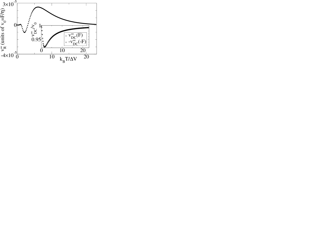
Figure 3: Ratchet current and stationary velocity (inset) as a function of temperature for the potential of amplitude $\Delta V$ depicted in Fig. 1. Weak dissipation is chosen with $\alpha=0.2$ and $\hbar\gamma=0.76\Delta V$. Driving is set to $FL=0.57\Delta V$.

for a two-harmonics potential. In Fig. 3, the driving is set to $FL=0.57\Delta V$, whereas in Fig. 4, the temperature is fixed to $k_{\text{B}}T=0.23\Delta V$. With $V_{1}=4V_{2}$, the untilted potential, depicted in Fig. 1, has a barrier height $\Delta V=2.2V_{1}$. We choose $\alpha=0.2$ and $\hbar\gamma=0.76\Delta V$. It means that the typical action is $\sqrt{2M\Delta VL^{2}}\approx 2\hbar$, and the dissipation rate $\gamma=\eta/M$ is about one-fourth of the classical oscillation frequency $\Omega_{0}=2\pi\sqrt{V_{1}/ML^{2}}$ in the untilted potential (weak dissipation). In this numerical application, none of the rates exceeds $0.05\gamma$ and  $0.08\omega_{\text{B}}$, which means that the duality relation is valid for this system. Moreover, the third-order rates stay at least one order of magnitude below the second-order ones. The ratchet current presents several reversals as a function both of the driving and the temperature. As expected for the small values of driving and dissipation used in Fig. 3, the stationary velocity is very close to the value of a free system $v_{0}=F/\eta$ at $T=0$, which corresponds to localization $v_{\text{TB}}^{\infty}\approx 0$ in the TB system note2 . Accordingly, $v_{\text{R}}^{\infty}\approx 0$ in this regime. The stationary velocity also tends to $v_{0}$ (dashed line in Fig. 4) for driving or temperatures much higher than the potential barrier, and the ratchet current vanishes correspondingly. If observed in experiments, this linear behavior would provide a direct estimation of dissipation.

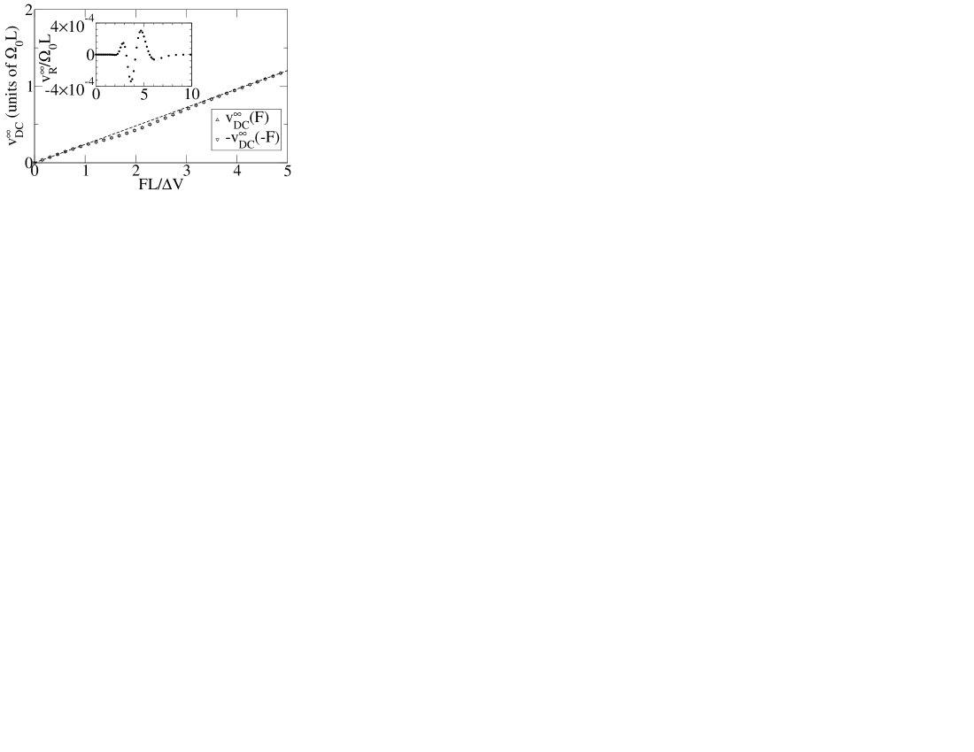
Figure 4: Stationary velocity and ratchet current (inset) as a function of driving for the potential of amplitude $\Delta V$ depicted in Fig. 1. The dashed line is the classical solution in the absence of potential. Weak dissipation is chosen with $\alpha=0.2$ and $\hbar\gamma=0.76\Delta V$. Temperature is set to $k_{\text{B}}T=0.076\Delta V$.

In conclusion, we obtained a duality relation yielding a tight-binding description of Brownian motion in a tilted ratchet potential. We demonstrated its application to investigate rectification of adiabatic driving and ground-state delocalization for weak dissipation.

References

(1)Appl. Phys. A 75, 167 (2002),
special issue on Ratchets and Brownian motors; P. Reimann, Phys. Rep. 361, 57 (2002);
R. D. Astumian and P. Hänggi, Phys. Today 55 (11), 33 (2002).