Shearing behavior of polydisperse media

Abstract

We study the shearing of polydisperse and bidisperse media with a size ratio of 10. Simulations are performed with a the two dimensional shear cell using contact dynamics. With a truncated power law for the polydisperse media we find that they show a stronger dilatancy and greater resistance to shearing than bidisperse mixtures. Motivated by the practical problem of reducing the energy needed to shear granular media, we introduce ”point-like particles” representing charged particles in the distribution. Even though changing the kinematic behavior very little, they reduce the force necessary to maintain a fixed shearing velocity.

1 Introduction

Granular media show a wide variety of phenomena and people tried to understand these phenomena using continuum mechanics. Parallel to that, computer models like Molecular Dynamics [1] or contact dynamics [2, 3, 4] are used to simulate granular media on the individual grain level. The application of external stress to a granular system leads to force chains. Along these chains the system carries the majority of the stress while there are regions with small or no stress. When the system is sheared, these chains break up and stress fluctuations can be observed [5, 6].

Dilatancy is one of the fundamental properties of granular media and first studies where done by Reynolds in 1885 [7]. Special interest lies in understanding dilatancy due to the shearing of granular materials. Here experiments on granular media immersed in water, [8], sheared granular layers, [9] and two-dimensional granular Couette experiments [10] contributed many insights. On the other hand computational physics helps to study these complex systems. Thompson and Grest [11] use molecular dynamics on disks while Tillemans and Herrmann [12] use polygons. Other numerical work was done by Lacombe et al. [13] and L tzel et. al. [14].

Recent work [15] compares results given by the Enskog equation and results from a MD for polydisperse granular fluids under shear. In the present studies we will focus on the shearing behavior of polydisperse mixtures. Therefore we compare it to a bidisperse mixture and study the changes subject to the introduction of point particles.

2 The model

First we will define different particle distributions and introduce our ”point-like particles”. Afterwards we give an overview over the simulation method including the procedure we used to initialize the system. Finally compaction and shearing of the system is explained.

2.1 Grains

We simulate a two-dimensional system of circular disks which we will refer to as ”grains”. We define the polydispersity $\Pi$ of our mixtures by:

$$\Pi=\frac{r_{max}}{r_{min}}$$ (1)

A bidisperse distribution contains particles of two different sizes. The radius of the large particles be $r_{max}$ while the radius of the small particles be $r_{min}$. To fully define this distribution we introduce the ratio $R$ between the number of big particles and the number of small particles by:

$$R=\frac{N(r_{max})}{N(r_{min})}$$ (2)

Here $N(r)$ is the number of particles of a given size $r$.

The polydisperse distribution is given by a truncated power law:

$$P(r)=a\cdot r^{-b}$$ (3)

Here $r$ is the radius of the particle, $b$ the exponent of the power law and $a$ a prefactor which is chosen such that $\int_{r_{min}}^{r_{max}}P(r)dr=1$, where $r_{min}$ and $r_{max}$ are the minimum and maximum radius in the distribution.

The mass $m$ of the grains is given by:

$$m=\frac{4}{3}\pi r^{3}$$ (4)

For resolving the grain-grain interactions we use contact dynamics where we have set the restitution coefficient $r_{c}$ to $0.2$. Additionally we use Coulumb friction, where the Coulomb force is defined by:

$$F_{C}=\mu F_{n}$$ (5)

We determine the tangential force $F_{T}$ necessary to reduce the tangential velocity $v_{t}$ of the contact to zero. In the case of sliding friction, $F_{T}$ is larger than $F_{C}$ and we reset it to $F_{C}$ before applying it to the contact. In the case of static friction, we apply $F_{T}$ as it is smaller than $F_{C}$.

2.2 Point-like particles

A point-like particle has a zero radius, zero mass and interacts with grains through the potential:

$$U(d)=\left\{\begin{array}[]{ll}kd_{r}\hat{d}^{-1}e^{-\alpha\hat{d}}+F_{0}\hat{d}+U_{0},&0<\hat{d}<1\\ 0,&\hat{d}\geq 1\end{array}\right.$$ (6)

Here $d_{r}$ is the interaction radius of the point-like particle and $\hat{d}=d/d_{r}$ is the dimensionless distance between the particle surfaces, where $d$ is the separation between the particle surfaces. Note that when $d>d_{r}$ the particles do not interact.

The first term in Eq. 6 is a screened long-range potential. This term contains two constants: $k$ determines the strength of the potential while $\alpha$ fixes how fast it decays with the distance. In this work, we fix $\alpha=3$ and adjust the range of the potential through $d_{r}$. The second and third terms are small, and added for numerical convenience. The constants $U_{0}$ and $F_{0}$ are chosen such that potential and force are continuous at $d=d_{r}$.

The repulsive force $F_{r}$ is just the gradient of the potential:

$$F_{r}(d)=-\frac{\partial U}{\partial d}=\left\{\begin{array}[]{ll}k\hat{d}^{-1}e^{-\alpha\hat{d}}(\hat{d}^{-1}+\alpha)-F_{0}&0<\hat{d}<1\\ 0&\hat{d}\geq 1\end{array}\right.$$ (7)

Point-like particles don’t contribute to the density of the system but exert a repulsive force $F_{r}$ on every particle closer than the distance $r_{r}$. As they have no mass and thus might experience infinite accelerations when using contact dynamics we use a different iteration scheme for calculating their motion. Before beginning a contact dynamics time step, each point-like particle is moved to a position where the net force on it vanishes. Then the forces exerted by the point-like particles on the other particles are computed, and the contact dynamics time steps proceeds normally.

2.3 Simulation Method

In this section we will explain the setup we used to investigate the shear behavior of particle mixtures immersed in a fluid. First we fill the shear cell with an initial configuration of particles then we compact this configuration and in the last stage we shear the system.

2.3.1 The shear cell

Figure 1: The shear cell with periodic boundaries. The length of the cell is $l$ and the actual hight of the lid is given by $h(t)$. While we shear the lid with the velocity $v$ we exert the normal force $F_{N}$ onto the lid.

Fig.1 shows the two dimensional shear cell. We apply periodic boundary conditions such that particles leaving the cell to the left will reenter on the right and vice versa. The length of the system is $l=10cm$ and we set the density of the particles to $\rho=10^{3}kg/m^{3}$. The bottom wall is fixed while on the top wall, the lid, we exert a force $F_{N}=100N$ in all simulations. The position of the lid is given by its height $h(t)$. After compaction we shear the lid with the velocity $v$.

In all simulations we turned off gravity.

2.3.2 Initialization

In order to obtain a high starting density we use a hierarchical initialization scheme. First we fill a separate reservoir with either the bidisperse or the polydisperse mixture. While filling the reservoir we calculate the area $V$ of all particles in the reservoir.

$$V=\sum_{i}^{n}\pi r_{i}^{2}$$ (8)

Here $r_{i}$ is the radius of the $i$th particle and $n$ is the number of particles in the reservoir. When $V$ becomes equal or greater than 70% of the shear cell volume we stop filling the reservoir. Next we change the indices of the $n$ particles in the reservoir such that $r_{1}>r_{2}>...>r_{n}$. Starting with the largest particle we consecutively take the next smaller particle and give it $I$ trials to find a random position in the shear cell where it does not overlap with any particle already present or the top and bottom wall. The value for $I$ is chosen high enough that all $n$ particles can be placed in the shear cell.

If point-like particles are used in the simulation they are put in next. We take $N_{p}$ point-like particles and give them $I_{p}$ trials for adsorption. As $r=0$ all $N_{p}$ point-like particles can be put into the system for a large enough $I_{p}$. During the initialization the strength of the potential is always set to $k_{i}=10^{-3}N$ and before we start shearing, $k$ is set to the wanted value. This makes it faster to reach our desired initial density when compressing as $k$ is greater of equal to $k_{i}$ in all our simulations.

When all particles have been placed in the shear cell, the initialization is complete.

When averaging over several simulation we always use the same $n$ grains and the same number $N_{p}$ of point-like particles in the reservoir but use a different seed for the random number generator responsible for choosing the positions of the particles. Thus the distribution of particle sizes remains exactly the same, only the initial configurations are different.

2.3.3 Compaction

The actual volume fraction $\Phi$ of the system is given by:

$$\Phi(t)=\frac{V}{lh(t)}$$ (9)

Starting from the initial configuration we want to reach a specific volume fraction $\Phi_{0}$ at which we start the shearing. To reach $\Phi_{0}$ we exert a fixed normal force $F_{N}$ on the lid and, in certain time intervals, we give the grains a random force in a random direction. Due to the force $F_{N}$ the system is compressed while the random forces break up arches and thus allow for better compaction. Additionally we turn off friction ($\mu=0$). As soon as the volume fraction $\Phi$ reaches the desired value $\Phi_{0}$ we stop the compaction, turn on friction ($\mu=0.3$) and start shearing.

2.3.4 Shearing

In the compacted system we determine the grains with a radius smaller than $2r_{min}$ and a distance smaller then $r_{min}/2$ away from the top and bottom wall and fix them to these walls. The position of the lid at the moment we start to shear is the reference height $h_{0}$. As we shear the lid with a constant velocity $v$, we measure the position $h$ of the lid and the force $F$ we need to exert on it to keep $v$ constant. We shear for at least 0.1 seconds in all simulations. For the slowest shear velocity the lid moves at least a distance $l/2$ in horizonal direction.

2.3.5 Particle contact detection

Now we will consider the detection of the particle contacts. A well know method is the ”linked cell” algorithm [16]. Here a grid of equal sized cells of side length $s$, the radius of the biggest particle, is put over the system and each particles is assigned to the cell in which its center lies in. In the next step the ”Verlet list”, containing pairs of particles whose separation is smaller than a certain threshold $d_{t}=s/2$, is created by determining contacts between the particles in one cell and those in the neighboring cells. With neighboring cells we refer to the nearest and next nearest neighbors. Thus a cell has eight neighbors in two dimensions. When creating the Verlet list it is sufficient to check only half of the neighbouring cells. If any particle travels further than $d_{t}$ the Verlet list is regenerated. When using this method for very polydisperse media, each cell will contain many small particles which will slow down the simulation as we put many unnecessary contacts into the Verlet list.

Figure 2: Grid created by the Quadtree

Figure 3: Generating a quadtree in two dimensions. Starting from the root cell on level $L=0$, we subdivide the space into $n=4$ subcells which are then on level $L=1$. As there are two particles in the upper right corner, this cell is again divided into 4 cells.

Therefore we use an alternative algorithm, namely the two dimensional quadtree, shown in Fig. 2. The quadtree is a grid with variable cell size. It is finer where there are many small particles while it is coarse around big particles. The creation of the grid starts with the root cell, which contains the whole system and uses the following rule: If a cell contains more than one particle, subdivide it into $n$ smaller cells and transfer each particle into that new cell where its center lies. Continue for the new cells if they contain more than one particle. The number of new cells $n$ depends on the dimension $D$ and is given by: $n=2^{D}$.

Fig. 3 shows an example in two dimensions. Starting from the root cell on level $L=0$, we subdivide the space into $n=4$ subcells which are then on level $L=1$. As there are two particles in the upper right cell, this cell is again divided into 4 cells. For practical reasons we define a maximum depth level $L_{max}$ at which we stop subdividing a cell even if it contains more than one particle. With $d_{t}=\frac{l}{2^{L_{max}+1}}$, half the size of the smallest cell, a large $L_{max}$ results in a smaller Verlet list but we need to update it more often as $d_{t}$ becomes smaller.

We use the quadtree to create the Verlet list. A contact is added if the separation between two particles is smaller than $d_{t}$, which is half the size of the smallest cell. If a particle travels further than $d_{t}$ we have to regenerate the quadtree and update the Verlet list. To create the quadtree and determine the contacts added to the Verlet list, we need to know the following lists for each cell:

• list $\mathbb{A}$: particles belonging to this cell

• list $\mathbb{B}$: particles overlapping this cell

• list $\mathbb{N}$: neighboring cells

As the purpose of the last two lists is not evident, we will explain how they are used when building the Verlet list. First, we compile a seperate list of leaves, which are cells without subcells. Now recall that all particles are contained in the lists $\mathbb{A}$ of the leaves. If we would follow the linked cell algorithm we would create the Verlet list simply by checking the particles of each leaf with those in the neighbouring leaves. However, due to the polydispersity of the system we would miss several contacts. For instance, in Fig. 3, the contact between the big particle $a$, whose center lies in the lower left cell, and the small particle $b$ would be missed. This problem is solved by checking the list $\mathbb{B}$ of the neighboring cells as well. A second difficulty is that the quadtree is an adaptive structure that gives a different neighbor list each time it is created. As the generation on the fly would be too costly we store $\mathbb{N}$ during the generation of the quadtree.

3 Method of analysis

The shearing is characterized by three parameters, the angle of dilatancy $\Psi$ and the saturation dilatancy $d_{s}$ which characterize the movement of the lid and the force $F$ needed to maintain the shearing motion.

3.1 Dilatancy

Figure 4: Expansion $\Delta h(t)$ over the shear distance $s$. The left picture shows a polydisperse mixture and the right a bidisperse mixture with $R=1/45$. In both cases, $\Phi=0.887$, $v=1.5\textrm{m/s}$ and $\Pi=1/45$. For small values of $s$, $\Delta h(t)$ increases almost linearly. For larger values of $s$, $\Delta h(t)$ fluctuates around a saturation value. The straight lines show the fits used to obtain $\Psi$ and $d_{s}$ from $h(t)$.

Fig. 4 shows $\Delta h(t)=h(t)-h_{0}$ over $s=vt$ for a polydisperse and a bidisperse system. The expansion $\Delta h(t)$ tells us how far the lid moved from its starting position $h_{0}$ while the shear distance $s$ is the distance the lid moved horizontally. One can identify two different regimes. For small values of $s$, $\Delta h(t)$ increases almost linearly. For larger values of $s$, $\Delta h(t)$ fluctuates around a saturation value.

One can characterize this behavior by the angle of dilatancy $\Psi$ and the saturation dilatancy $d_{s}$. Just after the onset of shearing, the height of the lid can be described by

$$h(t)=h_{0}+vt\tan\Psi.$$ (10)

Therefore, $\Psi$ can be determined by fitting a straight line to $h(t)$ for small $t$ and extracting the slope of the line. Specifically, we do a least squares fit for the height using the points where $s<0.002\textrm{m}$. Thus we make sure we only measure the beginning of the shearing. Sometimes, the lid first descends before rising. In this case, we begin the fit when the lid is at its lowest position, and continue it until $s$ has increased by $0.002\textrm{m}$.

Dilatancy is a measure of how much a medium expands when subject to shear. Therefore the saturation dilatancy $d_{s}$ is calculated using

$$d_{s}=h_{s}/h_{0}.$$ (11)

With $h_{s}$, the average height the lid is assumed to reach for long times and $h_{0}$, the height of the lid before we start shearing. In our simulations, it was often difficult to determine $h_{s}$ because it was often not clear that the height had saturated before the simulation had ended. We obtained values for $h_{s}$ by taking the average over $\Delta h(t)=h(t)-h_{0}$ for $t>0.05$ seconds.

3.2 Shearing force

Figure 5: The horizontal force $F(t)$ divided by the normal force $F_{N}$, as a function of the shear distance $s$, for the simulations shown in Fig. 4. Again, the polydisperse system is displayed on the left while the right picture shows the bidisperse one. When the shearing started, the force is high but decreases over time until it fluctuates around a saturation force $F_{s}$. Ten simulations were averaged together to obtain these curves. The straight lines show the result of fitting the force to the function in Eq. 12.

Fig. 5 shows the horizontal force $F(t)$ divided by the normal force $F_{N}$, as a function of the shear distance $s$, for the simulations shown in Fig. 4. In order to maintain a constant shear velocity $v$ a force $F(t)$ must be exerted on the lid. When the shearing started, the force is high but decreases over time until it fluctuates around a saturation force $F_{s}$. We are only interested in the resulting saturation force and thus need a method to cut off the part of the data where the force is still decreasing. This we did by fitting:

$$F(t)=\left\{\begin{array}[]{ll}F_{0}+\alpha vt&t<t_{*}\\ F_{s}&t\geq t_{*}\\ \end{array}\right.$$ (12)

Here $F_{0}$ is the force necessary to start the shearing with velocity $v$ and $\alpha$ is the slope telling us how fast the shearing force approaches its saturation value which it reaches at time $t_{*}$. The three parameters $F_{0}$, $\alpha$, and $F_{s}$ are extracted by fitting the observed force to Eq. 12. Typically $F_{s}\approx\mu F_{N}$ and $F_{0}$ is at the maximum twice as big as $F_{s}$ while $\alpha\approx 1000-25000\textrm{N/m}$.

4 Results

We first compare the shearing behavior of bidisperse and polydisperse mixtures and in the second part we will investigate how the introduction of point-like particles changes this behavior for polydisperse mixtures.

4.1 Bidisperse and polydisperse mixtures

We investigated two bidisperse mixtures and a polydisperse one. In the polydisperse mixture, the sizes are distributed according to Eq. 3 with $b=3.5$. For the bidisperse mixtures we have $R=1/45$ and $R=1/60$ [see Eq. 2]. In both bidisperse mixtures, $\Pi=10$ ($r_{min}=0.1\textrm{cm}$, $r_{max}=1\textrm{cm}$). The simulations were done with either 575 (polydisperse), 690 ($R=1/45$), or 732 ($R=1/60$) particles.

We examined each mixture at two or three initial densities. All mixtures were studied at $\Psi=0.887$ and $0.876$. In addition the bidisperse mixtures were examined at $\Psi=0.911$. For each mixture-density pair, ten different samples were prepared and the shearing velocity was set to three different values: $v=0.5,1.5,4.5\textrm{m/s}$. The time series from each group of ten simulations were averaged together to obtain the shearing parameters.

Figure 6: Dilatancy angles $\Psi$ for bidisperse and polydisperse mixtures, as a function of the initial shear rate $v/h0$ . The empty symbols correspond to polydisperse mixtures; the large, filled symbols correspond to a bidisperse mixture with $R=1/45$, and the small, filled symbols to a bidisperse mixture with $R=1/60$. The squares indicate results for an initial solid fraction $\Phi_{0}=0.911$, the circles $\Phi_{0}=0.887$ and the triangles $\Phi_{0}=0.876$. The highest density ($\Phi_{0}=0.911$) could only be obtained with the bidisperse mixtures. The angle of dilatancy increases with shearing velocity and density but is roughly three times smaller for bidisperse mixtures than for polydisperse ones.

In Fig. 6, we show the angle of dilatancy $\Psi$ over the initial shear rate $v/h_{0}$ for the different simulations we performed. Some trends can be seen. The angle of dilatancy increases with shearing velocity and density but is roughly three times smaller for bidisperse mixtures than for polydisperse ones. On the other hand, at the maximum density ( $\Phi_{0}=0.911$), the bidisperse mixture’s angle approaches those of the polydisperse mixture. Note that this density could not be obtained for the polydisperse mixture.

Figure 7: Saturation dilatancy $d_{s}$ for polydisperse and bidisperse particles. The symbols are the same as those used in Fig 6. As for the angle of dilatancy the saturation dilatancy increases with velocity and density and is for polydisperse particles greater then for bidisperse mixtures. Note the negative dilation for the bidisperse system displayed by the large filled triangles.

The saturation dilatancy for the systems we studied is shown in Fig. 7. Here we plot $d_{s}$ over the initial shear rate. As for the angle of dilatancy the saturation dilatancy increases with velocity and density and is for polydisperse particles greater then for bidisperse mixtures. An important difference is the fact that for the lowest initial density only bidisperse mixtures exhibit negative dilation. This means that the height $h_{s}$ at the end of shearing is lower than $h_{0}$ at the beginning. This occurs because the small particles do not fill all the spaces between the large particles during the preparation of the sample. When the shearing begins, there can be large voids between the big particles. As the shearing proceeds, the large particles move relative to one another, the voids are opened up, and quickly filled with small particles. The voids never re-form, leading to a permanent decrease in the height of the lid.

Figure 8: The saturation value of the force $F_{s}$ , divided by the imposed normal force $F_{N}$, over the initial shear rate for polydisperse and bidisperse particles. The symbols are the same as those used in Fig. 6. Note that all values are close to the Coulomb friction ratio $\mu=0.3$ used in the simulations. The polydisperse particles have a force that is roughly 30% higher than the bidisperse ones. The force is roughly independent of the initial density. Surprisingly, it decreases slightly with velocity, at least between $v=0.05$ and $v=0.15$.

In Fig. 8, we show the saturation force $F_{s}$ divided by $F_{N}$ over the initial shear rate for the different series of simulations. The polydisperse particles have a force that is roughly 30% higher than the bidisperse ones. The force is roughly independent of the initial density. Surprisingly, it decreases slightly with velocity, at least between $v=0.5\textrm{m/s}$ and $v=1.5\textrm{m/s}$. This differs from other cases, where the force is always observed to increase with shearing velocity [12]. However, that work concerns flow of approximately monodisperse polygons, whereas we have studied disks. The decrease in $F_{s}$ can be understood as a consequence of dilatancy. At higher velocities, dilatancy increases and thus making it easier to shear.

4.2 Point-like Particles

In this section we systematically study how the shearing parameters for a polydisperse mixture change when point-like particles are added. Again, the size distribution in the polydisperse mixture follows Eq. 3 with an exponent $b=3.5$.

For the point-like particles there are three parameters we can change. The first two are the strength $k$ and the range of the repulsive force $d_{r}$ in the repulsive potential in Eq. 6. The third parameter $A=\frac{N(\textrm{point-like})}{N(\textrm{grains})}$ gives the number of point-like particles, divided by the number of non point-like particles. We set the following values for these parameters: $A=1,2$, $d_{r}=\frac{1}{5}r_{max},\frac{2}{5}r_{max}$ and $k=2,5,10\times 10^{-3}N$ For all simulations we set $\Phi=0.882$ and the shearing velocity to $v=1.5\textrm{m/s}$. In both mixtures we have $\Pi=10$ and $r_{min}=0.11\textrm{cm}$, $r_{max}=1.1\textrm{cm}$. For each set of these three parameters, ten simulations with different initial configurations were done and averaged together. For some systems we even set the strength of the potential to $k=20,50,100\times 10^{-3}N$.

In Fig. 9 we show the expansion $\Delta h(t)$ over the shear distance $s$ for a polydisperse and the same polydisperse system with one point-like particle added for every grain ($A=1$). The straight lines show the fits used to obtain $\Psi$ and $d_{s}$. One can see that the presence of the point-like particle changes the curve very little.

Figure 9: Expansion $\Delta h(t)$ over the shear distance $s$. The left picture shows the polydisperse mixture, the right picture shows the same mixture, with one point-like particle added for every grain ($A=1$). In both cases, $\Phi_{0}=0.882$ and $v=1.5\textrm{m/s}$. The repulsive potential has a strength of $k=10^{-3}N$ and interaction distance $d=0.22\textrm{cm}$ ($1/5$ the radius of the largest particles). Ten simulations were averaged together to obtain these curves. The straight lines show the fits used to obtain $\Psi$ and $d_{s}$. One can see that the presence of the point-like particle changes the curve very little.

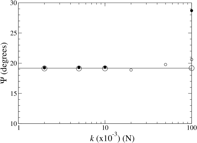
Figure 10: Dilatancy angles $\Psi$ for polydisperse mixtures with and without point-like particles, as a function of the the strength of the repulsive potential $k$. The horizontal line shows the value of $\Psi$ obtained when there are no point-like particles. The small circles correspond to repulsive particles with a small interaction radius ($1/5$ the radius of the largest particle) and large circles correspond to a large interaction radius ($2/5$ of the largest particle). The empty symbols represent simulations with equal numbers of repulsive particles and grains ($A=1$); the filled symbols represent simulations when the number of repulsive particles has been doubled ($A=2$). In all cases, the density is $0.882$ and the shearing velocity is $1.5\textrm{m/s}$. The addition of point-like particles does not cause much change. The observed angles vary by about $1$ degree from the value found without point-like particles.

In Fig. 10, we plot $\Psi$ over $k$ for the different types and numbers of point-like particles. One data point stands out from the rest: ($\Psi\approx 29^{\circ}$, $k=100\times 10^{-3}N$, $A=2$). For the moment, we will exclude it from our discussion and treat it in a special section, Sec. 4.2.1. Except for this one series of simulations, the addition of point-like particles does not cause much change. The observed angles vary by about one degree from the value found without point-like particles. Compared with the changes we discussed in the previous section the changes due to the point-like particles are one magnitude smaller then when changing the shear velocity or the initial density.

A very surprising feature of the shearing behavior extracted from Fig. 10 is that point-like particles with a large distance of interaction cause less change than particles with a small distance. (Compare the large and small empty circles at $k=100\times 10^{-3}N$.)

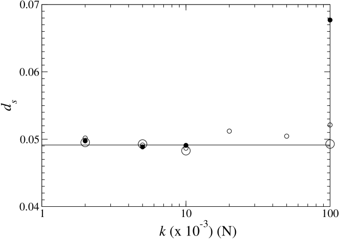
Figure 11: Saturation dilatancy $d_{s}$ for mixtures with different concentrations of point-like particles. The symbols are the same as those used in Fig. 10. The presence of point-like particles changes the behavior of the mixture very little.

The saturation dilatancy $d_{s}$ over the strength $k$ of the potential for the systems studied is shown in Fig. 11. The data are very similar to those discussed above. The simulations with $k=100\times 10^{-3}N$ and $A=2$ are widely separated from all the others. Except for this one data point, the presence of point-like particles changes the behavior very little. When point-like particles are added, the dilatancy changes by at most $0.003$. The changes due to the change in density or shear rate, observed in the previous section were seven time larger. In Fig. 12 we show the horizontal force $F(t)$ divided by the normal force $F_{N}$, as a function of the shear distance $s$, for the simulations shown in Fig. 9.

Figure 12: The horizontal force $F(t)$ divided by the normal force $F_{N}$, as a function of the shear distance $s$, for the simulations shown in Fig. 9. The left picture shows the polydisperse mixture and the right picture shows the same simulation with point-like particles ($A=1$ and $k=100\times 10^{-3}N$. In both cases, $\Phi_{0}=0.882$ and $v=1.5\textrm{m/s}$. Ten simulations were averaged together to obtain these curves. The straight lines show the result of fitting the force to the function in Eq. (12).

Figure 13: The saturation value of the force $F_{s}$, divided by the imposed normal force $F_{N}$, for systems with different concentrations of point-like particles. The symbols are the same as those used in Fig. 10. Note that $F/F_{N}\approx\mu$ when $k$ is small. When short-range point-like particles are added to the polydisperse mixture (with $d_{r}=r_{\mathrm{max}}/5$, the small circles in the figure), the force decreases substantially. At large $k$, the force is reduced to half of its original value, or very nearly removed, depending on how many point-like particles are added.

In Fig. 13, we show the saturation force $F_{s}$ over $F_{N}$ when the lid fluctuates about its saturation height $h_{s}$ for the different series of simulations. This time, the point-like particles change the behavior of the mixture. When short-range point-like particles are added (with $d_{r}=r_{\mathrm{max}}/5$, the small circles in the figure), the force decreases substantially. At large $k$, the force is reduced to half of its original value, or very nearly removed, depending on how many point-like particles are added.

Surprisingly, adding the long-range particles does not reduce the force at all. This continues the general trend observed in the previous discussion, where we saw that the particles with a large interaction distance did not have much effect. One possible reason for this is that when $d_{r}$ is small, the grains feel only those point-like particles that occupy the neighboring pore spaces. The force exerted on the grains is thus tightly connected to the geometry of the surrounding particles, and this force is such that it reduces the friction between the grains. When $d_{r}$ is large, grains interact with point-like particles in many different regions, and the resulting forces are no longer so closely related to the geometry of the neighboring particles.

4.2.1 Behavior at large $k$ and $A$

In Fig. 10, we observed for large $k$ and $A$ a very high angle of dilatancy (nearly $30^{\circ}$ compared with all the other points near $20^{\circ}$.), and in Fig. 11 a very high saturation dilatancy (roughly $40\%$ more than any other point). In addition, the force needed to shear this mixture is very low – only $10\%$ of the mixture without point-like particles. This last result suggests that the point-like particles are carrying a significant fraction of the weight of the lid. This would explain the very high dilatancy. Note that all the samples are prepared by compressing mixtures with $k=10^{-3}N$. Then, when the shearing starts, $k$ is set to its final value. If $k$ is very large and the point-like particles are numerous, the mixture will expand not due to shearing, but simply because the point-like particles push against each other with enough force to lift up the lid.

This explanation has been confirmed by simulations of unsheared systems. The system is prepared as before, but is not sheared. When $k=100\times 10^{-3}N$ and $A=2$, we observe a substantial dilation ($d_{s}\approx 0.28$) due only to the repulsive potential of the point-like particle. On the other hand, when $k=100\times 10^{-3}N$ and $A=1$, no such dilation is observed. We conclude, therefore, that the point at $k=100\times 10^{-3}N$ and $A=2$ is in a different regime from the other points.

4.2.2 Dependence on polydispersity

All of the above results were obtained with a polydisperse mixture described by a power law exponent $b=3.5$ [see (3)]. We also tried mixtures with $b=1.3$. Point-like particles with $d_{r}=0.022$ and $2\times 10^{-3}N\leq k\leq 100\times 10^{-3}N$ were added. No significant change in the dilatancy or force is observed, even for the largest values of $k$. This may be because there are fewer small grains, and the pore spaces are much larger. The point-like particles can then stay in the middle of this pore spaces and interact only weakly with the grains.

5 Conclusion

The findings of this study can be summarized by saying that the polydisperse mixtures show stronger dilatancy and a greater resistance to shearing than the bidisperse mixtures. At constant density, the angle of dilatancy, the saturation dilatancy, and the force needed to maintain the shearing were all greater for polydisperse particles. However, this simple conclusion is complicated by the fact that higher densities were easier to obtain with bidisperse mixtures. When bidisperse mixtures are very dense, their angle of dilatancy and saturation dilatancy is similar to polydisperse systems at lower densities (although the shearing force remains significantly smaller).

Adding repulsive particles to a sheared polydisperse mixture of grains changes the kinematic behavior of the mixture very little, but the dynamic behavior shows a reduction in the forces. By ”kinematic” we mean those properties that concern the movement of the mixture – the angle of dilatancy and the saturation dilatancy. By ”dynamic” behavior, we mean the force necessary to maintain a fixed shearing velocity. This finding is complicated by two additional observations. First, particles with a large interaction distance cause little change, in spite of exerting larger forces. The second observation is that it is possible to get dramatic changes in the kinematic behavior when there are many point-like particles with strong repulsive forces.

In general we can say that the point-like particles lead to a lubrication effect which reduces the force necessary to shear the system. But one has to be careful not to add too many point-like particles. If the number of point-like particles becomes too large, they will build a network that carries most of the load and leads to a strong dilation after the initialization. For future work it might be interesting to see how the lubrication effect changes when using different normal forces on the lid.

References

References

- [1] S.Luding. Stress distribution in static two-dimensional granular model media in the absence of friction. Physical Review E, 55(4):4720–4729, 1997.
- [2] Farhang Radjai and Lothar Brendel. Nonsmoothness, indeterminacy, and friction in two-dimensional arrays of rigid particles. Physical Review E, 54(1):861–873, 1996.
- [3] Farhang Radjai, Michael Jean, Jean-Jaques Moreau, and St phane Roux. Force Distribution in Dense Two-Dimensional Granular Systems. Physical Review Letters, 77(2):274–277, 1996.
- [4] J.J. Moreau. Lecture Notes in Applied and Computational Mechanics, chapter Novel Approaches in Civil Engineering. 2004.
- [5] Brian Miller, Corey O’Hern, and R. P. Behringer. Stress Fluctuations for Continuously Sheared Granular Materials. Physical Review Letters, 77(15):3110–3113, 1996.
- [6] Daniel W. Howell and R. P. Behringer. Fluctuations in granular media. Chaos, 9(3):559–572, 1999.
- [7] O. Reynolds. On the dilatancy of media composed of rigid particles in contact. Philo. Mag., 20:469, 1885.
- [8] J. G minard, W. Losert, and J. Gollub. Frictional mechanics of wet granular material. Physical Review E, 59(5):5881–5890, 1999.
- [9] S. Nasuno, A. Kudrolli, and J. P. Gollub. Friction in Granular Layers: Hysteresis and Precursors. Physical Review Letters, 79(5):949–952, 1997.
- [10] C. T. Veje, Daniel W. Howell, and R. P. Behringer. Kinematics of a two-dimensional granular Couette experiment at the transition to shearing. Physical Review E, 59(1):739–745, 1999.
- [11] P. Thompson and G. Grest. Granular Flow: Friction and the Dilatancy Transition. Physical Review Letters, 67(13):1751–1754, 1991.
- [12] HJ Tillemans and H.J. Herrmann. Simulation deformations of granular solids under shear. Physica A, 217:261–288, 1995.
- [13] F. Lacombe, S. Zapperi, and H.J.Herrmann. Dilatancy and friction in sheared granular media. Eur. Phys. J. E, 2(2):181–189, 2000.
- [14] M.L tzel, S.Luding, H.J. Herrmann, D.W. Howell, and R.P. Behringer. Comparing simulation and experiment of a 2d granular Couette shear device. Eur. Phys. J. E, 11:325–333, 2002.
- [15] James F. Lutsko. The rheology of dense, polydisperse granular fluids under shear. Condmat, (0407100), 2004.
- [16] M.P.Allen and D.J.Tildesley. Computer Simulation of Liquids. Oxford University Press, Oxford, 1987.