Inelastic quantum tunneling through disordered potential barrier

Abstract

The effect of inelastic scattering on quantum tunneling through a rectangular potential barrier, of length $L$, containing randomly distributed impurities, is considered. It is shown that, despite the fact that the inelastic transition probability $\mathcal{T}_{\mathrm{inelastic}}$ is exponentially small, it may be greater than that of the elastic in the out of resonance conditions for some energy interval $\triangle E$ (the energy of the incident particle is far from the spectrum of the random Hamiltonian). The asymptotic of the tunnelling transition probability for various impurity configurations are found and the energy interval $\triangle E$ where $\mathcal{T}_{\mathrm{elastic}}\sim\exp(-L/L^{*})\lesssim\mathcal{T}_{\mathrm{inelastic}}$ is determined.

I Introduction

Due to advances in manufacturing techniques of semiconductor devices, that make it possible to create small tunnel junctions, and the need to understand fundamental conduction processes in order to improve these devices, quantum-mechanical tunneling of electrons through single, double or multi-barriers disordered resonant tunneling structure, is in the focus of physical interest Ref. LGP -FrelYurk and Misc1 -Misc2 . The most important peculiarity of these systems is that some impurity configurations may increase the tunneling probability dramatically. At the same time, the change of any single localized state will change the magnitude of the resonant transmission coefficient or even destroy the conditions needed for the resonant tunneling. There is the general belief that resonant tunneling via a single localized state (or a single quantum well) can dominate the whole tunneling process. Assuming this, the resonant tunneling through the whole system can approximately be treated using the resonant tunneling via a single localized state. Then, the Breit-Wigner formula is postulated to express the transmission coefficient as

$$\mathcal{T}(E)=\frac{\Gamma_{L}\Gamma_{R}}{(E-E_{0})^{2}+(\Gamma_{L}/2+\Gamma_{R}/2)^{2}}.$$ (1)

Here $E_{0}$ is the energy of the localized state and $\Gamma_{L}$, $\Gamma_{R}$ are leak rates of an electron from the localized state to left and right leads respectively, taken as $\Gamma_{L}\propto\exp(-2x/L_{\ell})$ and $\Gamma_{R}\propto\exp(-2(L-x)/L_{\ell})$, where $L$ is barrier length, $x$ is the position of impurity center and $L_{\ell}$ the localization length. The standard frameworks for the description of transport through a mesoscopic system are the Landauer-Buttiker formula, methods of random-matrix theory and Kubo’s formula Ref.LK ; KeldyshApproach ; Beenakker . Here we apply transfer matrix techniques, at first suggested in Ref.LK , with some generalization for inclusion of inelastic processes.

When the energy of incident particle is far from the spectrum of the random Hamiltonian, which describes the barrier with impurities, than we are not in the resonant conditions for tunneling. The Breit-Wigner formula is not applicable any more and the transition probability is exponentially small $\mathcal{T}(E)\propto\exp(-L/L^{*})$ with $L^{*}=\hbar/\sqrt{2m(U-E)}$ where $U$ barrier hight and $L$ barrier length. The situation changes when inelastic processes are taken into account which is relevant for low temperatures when electron-phonon collisions become sufficiently inelastic. The incident particle, by emission or absorbtion of a phonon, may be trapped into the resonant level with subsequent resonant tunneling. The probability of the inelastic scattering is exponentially small so that total tunneling probability is also exponentially small but it turns out that in some energy interval, $\triangle E=|E-E_{0}|$, the inelastic tunneling probability exponentially large compared to the elastic one in the regimes out of resonance. The last statement may be summarized in the following sequence of inequalities $\mathcal{T}^{\mathrm{res}}_{\mathrm{elastic}}(E\sim E_{0})\sim 1\gg\mathcal{T}(E)_{\mathrm{inelastic}}\gtrsim\exp(-L/L^{*})$. The aim of this work is to find out the energy interval $\triangle E$ when $\mathcal{T}(E)_{\mathrm{inelastic}}\gtrsim\exp(-L/L^{*})$ and investigate the energy dependence of tunneling probability in that interval for various configurations of impurity centers.

II Formalism

In this section we consider the tunneling of the quantum particle with the energy $E$ through the rectangular barrier with ingrained in it randomly distributed impurities. In the case of short-range point-like impurities, randomly arranged in the points $z_{j}$ $(j=1,2,\ldots,N)$, the impurity potential has the form

$$U(x)=U+K\sum_{j=1}^{N}\delta(x-z_{j}),\quad 0<z_{j}<L$$ (2)

so that electrons are described by the single-particle Hamiltonian

$$\hat{H}_{0}=-\frac{\hbar^{2}}{2m}\frac{\mathrm{d}^{2}}{\mathrm{d}x^{2}}+U+K\sum_{j=1}^{N}\delta(x-z_{j})$$ (3)

and interact with the phonon bath maintained in the thermal equilibrium through Frölich-like electron-phonon Hamiltonian. By introducing new variables $\kappa^{2}=2m(U-E)/\hbar^{2}$, $\mathcal{K}=2mK/\hbar^{2}$ and $k^{2}=2mE/\hbar^{2}$ we arrive at the Schrödinger equation

$$\frac{\mathrm{d}^{2}\Psi}{\mathrm{d}x^{2}}-\kappa^{2}\Psi=\mathcal{K}\sum_{j=1}^{N}\delta(x-z_{j})$$ (4)

with subsequent solutions of superposition the incident and reflected wave at $x<0$ and transmitted wave at $x>L$ in the form

$$\Psi(x)=\exp(\mathrm{i}kx)+r\exp(-\mathrm{i}kx),\quad x<0,$$ (5a)

$$\Psi(x)=t\exp(\mathrm{i}k^{\prime}(x-L)),\quad x>L.$$ (5b)

where $r$ – reflection and $t$ – transmission coefficients. Assuming the continuity of wave function and it derivative at the boundaries of the barrier we have following boundary conditions

$$\Psi(0)+\frac{\Psi^{\prime}(0)}{\mathrm{i}k}=2,\quad\frac{\Psi^{\prime}(L)}{\Psi(L)}=\mathrm{i}k^{\prime}.$$ (6)

In the above defined variables the the barrier transmittancy $\mathcal{T}$ can be presented as

$$\mathcal{T}(E,\Gamma_{N})=|t|^{2}=|\Psi(L)|^{2}.$$ (7)

and it depends on the energy $E$ of incident particle, number of the impurity centers $N$ and the configuration of impurities through the phase volume $\Gamma_{N}=\{z_{j}\}$. At this point it is convenient to introduce new notation for description the particle dynamics. Instead of the single wave function $\Psi(x)$ we introduce the vector-wave function

$$\hat{\Psi}(x)=\left(\begin{array}[]{c}\psi_{-}(x)\\ \psi_{+}(x)\end{array}\right)$$ (8)

such that

$$\Psi(x)=\psi_{-}(x)+\psi_{+}(x),\ \Psi^{\prime}(x)=\kappa(\psi_{-}(x)-\psi_{+}(x)).$$ (9)

Above definitions imply that the functions $\psi_{-}(x)$ and $\psi_{+}(x)$ satisfy the following equation

$$\frac{\mathrm{d}\psi_{\pm}}{\mathrm{d}x}=\pm\kappa\psi_{\pm}$$ (10)

everywhere, except the points $z_{j}$ so that

$$\frac{\mathrm{d}\hat{\Psi}(x)}{\mathrm{d}x}+\hat{A}\hat{\Psi}(x)=\frac{\mathcal{K}}{2\kappa}\hat{B}\sum_{j=1}^{N}\delta(x-z_{j})\hat{\Psi}(z_{j})$$ (11)

where

$$\hat{A}=\left(\begin{array}[]{cc}\kappa&0\\ 0&-\kappa\end{array}\right),\quad\hat{B}=\left(\begin{array}[]{cc}1&1\\ -1&-1\end{array}\right)$$ (12)

and subsequent new boundary conditions

$$\psi_{+}(0)(k/\kappa-\mathrm{i})+\psi_{-}(0)(k/\kappa+\mathrm{i})=2k/\kappa,$$ (13a)

$$\psi_{+}(L)(k^{\prime}/\kappa+\mathrm{i})+\psi_{-}(L)(k^{\prime}/\kappa-\mathrm{i})=0.$$ (13b)

Starting from now we can construct the scattering matrix $\hat{S}$ that ”carries” solution through the region $0<x<L$ from the right to the left boundary of the barrier:

$$\hat{\Psi}(0)=\hat{S}\hat{\Psi}(L),$$ (14)

$$\hat{S}=\hat{G}(z_{1})\hat{T}_{1,2}(z^{-}_{1}|z^{+}_{1})\hat{G}(z_{2}-z_{1})\ldots$$ (15)

$$\ldots\hat{T}_{N-1,N}(z^{-}_{N}|z^{+}_{N})\hat{G}(L-z_{N})$$

where $\hat{G}(x)$ is the free propagator that carries solution from right to left into the region free from the scattering centers

$$\hat{G}(x)=\left(\begin{array}[]{cc}\exp(\kappa x)&0\\ 0&\exp(-\kappa x)\end{array}\right)$$ (16)

and $\hat{T}$ is the matrix that propagates solution through the scattering center

$$\hat{T}_{j,j+1}(z^{-}_{j}|z^{+}_{j})=\frac{1}{2}\left(\begin{array}[]{cc}1+\frac{\kappa_{j+1}+\mathcal{K}}{\kappa_{j}}&1-\frac{\kappa_{j+1}-\mathcal{K}}{\kappa_{j}}\\ {}\hfil&{}\hfil\\ 1-\frac{\kappa_{j+1}+\mathcal{K}}{\kappa_{j}}&1+\frac{\kappa_{j+1}-\mathcal{K}}{\kappa_{j}}\end{array}\right)$$ (17a)

$$\hat{\Psi}(z_{j}-0)=\hat{T}_{j,j+1}(z^{-}_{j}|z^{+}_{j})\hat{\Psi}(z_{j}+0).$$ (17b)

Also we introduce following two vectors

$$f=\frac{1}{2}\left(\begin{array}[]{c}1+\mathrm{i}\kappa/\mathcal{K}\\ 1-\mathrm{i}\kappa/\mathcal{K}\end{array}\right),\quad g=\frac{1}{2}\left(\begin{array}[]{c}1+\mathrm{i}\mathcal{K}/\kappa^{\prime}\\ 1-\mathrm{i}\mathcal{K}/\kappa^{\prime}\end{array}\right).$$ (18)

that make it possible to present the transition probability in the very compact form

$$\mathcal{T}_{N}(E,\Gamma_{N})=\int\frac{W(E,E^{\prime})}{|(f,\hat{S}g)|^{2}}\mathrm{d}E^{\prime}$$ (19)

where function $W(E,E^{\prime})$ represents the probability of the electron transition from the quantum state with the energy $E$ into quantum state with the energy $E^{\prime}$ as the result of electron-phonon interaction, which may be found from linearized kinetic equation

$$W(E,E^{\prime})=W^{+}(E,E^{\prime})+W^{-}(E,E^{\prime}),$$ (20a)

$$W^{\pm}(E,E^{\prime})=\int|M_{q}|^{2}\frac{1-n_{F}(E^{\prime})}{1-n_{F}(E)}\frac{\delta(k(E)-\kappa(E^{\prime})\mp q)}{v(E^{\prime})}$$ (20b)

$$\times[(N_{q}+1)\delta(E-E^{\prime}-\hbar\omega)+N_{q}\delta(E-E^{\prime}+\hbar\omega)]\frac{\mathrm{d}q}{2\pi}$$

where $"\pm"$ correspond to emission and absorption of the phonon, $M_{q}$ – matrix element of the electron-phonon interaction, $N_{q}$ and $n_{F}$ – boson and fermion distribution functions and $\delta$-functions presents conservation laws of the momentum and the energy. Representation Eq. (19) is very useful because all information about particle dynamics in the barrier is included in $\hat{S}$ matrix, at the same time all information about boundary conditions lies in the vectors $f$ and $g$, and inelastic processes included in the function $W(E,E^{\prime})$.

Caring out integration in Eq. (20b), taking into account only valuable exponential factors and comparing $W$ to the elastic tunneling probability in the out of the resonance conditions $\propto\exp(-L/L^{*})$ we can find the energy interval $\triangle E$, where inequality $\mathcal{T}(E)_{\mathrm{inelastic}}\gtrsim\exp(-L/L^{*})$ is satisfied, which equals to

$$\triangle E\sim T\ln\left(\frac{1}{\exp(-L/L^{*})-\exp(-|E_{0}|/T)}\right)$$ (21)

where $T$ is temperature of the system and also assumed $L>L^{*}(|E_{0}|/T)$.

Analyzing properties of $\hat{S}$ matrix it is possible to show that maximum value for the tunneling probability occurs for some particular impurity configurations (resonant configurations). The conditions needed for $\mathrm{max}\{\mathcal{T}\}$

$$X(E,\Gamma_{N})=S_{11}-S_{22}\sim 1,\quad Y(E,\Gamma_{N})=S_{12}+S_{21}\sim 1$$ (22)

define this resonant configuration with the statistical weight

$$\Gamma^{\mathrm{res}}_{N}=\int_{|X(E,z_{1}\ldots z_{N})|\lesssim 1\atop|Y(E,z_{1}\ldots z_{N})|\lesssim 1}\mathrm{d}z_{1}\mathrm{d}z_{2}\ldots\mathrm{d}z_{N}.$$ (23)

It ratio to the full statistical weight of all possible configurations

$$\Gamma_{N}=\int_{0<z_{1}<\ldots<z_{N}<L}\mathrm{d}z_{1}\mathrm{d}z_{2}\ldots\mathrm{d}z_{N}=\frac{L^{N}}{N!}$$ (24)

gives the probability of the resonant configuration realization $P_{N}(E)$ for the given energy of the incident particle

$$P_{N}(E)=\frac{\Gamma^{\mathrm{res}}_{N}}{\Gamma_{N}}.$$ (25)

Averaged over all possible configuration, with the fixed number of impurities, the resonant transmittancy has the form

$$\mathcal{T}_{N}(E)\approx\frac{1}{\Gamma_{N}}\int_{\Gamma^{\mathrm{res}}_{N}(E)}\mathcal{T}_{N}(E,\Gamma_{N})\mathrm{d}\Gamma_{N}$$ (26)

and average value of transmittancy $\langle\mathcal{T}(E)\rangle$ for arbitrary number of impurities can be found by averaging $\mathcal{T}_{N}(E)$ with Poisson distribution function (under assumption of absence of correlation between impurities)

$$\langle\mathcal{T}(E)\rangle=\sum^{\infty}_{N=1}p_{N}\mathcal{T}_{N}(E),\quad p_{N}=(cL)^{N}\exp(-cL)/N!,$$ (27)

where $c$ is linear impurity concentration.

III Tunnel transparency $\mathcal{T}(E)$ of the disordered barrier

A) One impurity scattering center $N=1$: In what follows we have introduced new parameters $\epsilon=1+\mathcal{K}/2\kappa$, $\mathcal{L}=L\kappa$ and $\tau=\sqrt{2mL^{2}/(U-E)}$. The $\hat{T}$ and $\hat{S}$ matrices in the main approximation equals to

$$\hat{T}(z^{-}_{1}|z^{+}_{1})=\left(\begin{array}[]{cc}\epsilon+\omega\tau/2&-1-\omega\tau/2\\ 1-\omega\tau/2&2+\omega\tau/2\end{array}\right),$$ (28)

$$\hat{S}=\left(\begin{array}[]{cc}\epsilon\exp(\mathcal{L})\exp(\omega\tau(\mathcal{L}-\mathcal{Z}_{1}))&-\exp(-(\mathcal{L}-2\mathcal{Z}_{1}))\exp(-\omega\tau(\mathcal{L}-\mathcal{Z}_{1}))\\ \exp(\mathcal{L}-2\mathcal{Z}_{1})\exp(\omega\tau(\mathcal{L}-\mathcal{Z}_{1}))&2\exp(-\mathcal{L})\exp(-\omega\tau(\mathcal{L}-\mathcal{Z}_{1}))\end{array}\right).$$ (29)

The transmission probability has the form

$$\mathcal{T}_{1}(E,\Gamma_{N=1})\approx\frac{1}{1+\sinh^{2}[(\mathcal{L}-2\mathcal{Z}_{1})+\omega\tau(\mathcal{L}-\mathcal{Z}_{1})]+\frac{1}{4}\epsilon^{2}\exp(2\mathcal{L})\exp(2\omega\tau(\mathcal{L}-\mathcal{Z}_{1}))}\frac{e^{E/T}+1}{e^{E/T}+e^{\hbar\omega/T}}$$ (30)

and subsequently

$$\langle\mathcal{T}_{1}(E)\rangle\approx\frac{1}{\mathcal{L}}\int_{0}^{\mathcal{L}}\mathcal{T}_{1}(E,\Gamma_{N=1})\mathrm{d}\mathcal{Z}_{1}\approx\frac{2}{\mathcal{L}\epsilon^{2}}\ln\left[1+\epsilon^{2}\exp\left(4\mathcal{L}\frac{1+\omega\tau}{2+\omega\tau}\right)\right]\exp\left(-4\mathcal{L}\frac{1+\omega\tau}{2+\omega\tau}\right)\frac{e^{E/T}+1}{e^{E/T}+e^{\hbar\omega/T}}.$$ (31)

B) Two impurity scattering centers $N=2$: considering the case of two centers located in points $\mathcal{Z}_{1}$, $\mathcal{Z}_{2}>\mathcal{Z}_{1}$ it is convenient to introduce following quantities $\eta=\mathcal{Z}_{2}-\mathcal{Z}_{1}$ – relative distance between centers and $\zeta=(\mathcal{L}-\mathcal{Z}_{2})-\mathcal{Z}_{1}$ – asymmetry in the scattering centers configuration. Calculating elements of the scattering matrix $\hat{S}$ and then the $X$ and $Y$ functions form Eq. (22) we have

$$X(E,\Gamma_{N=2})=[\epsilon^{2}-\exp(-2\eta(1+\omega\tau))]\exp(\mathcal{L}-\mathcal{Z}_{1}\omega\tau)-$$ (32a)

$$-[4-\exp(2\eta(1+\omega\tau))]\exp(-\mathcal{(}L))\exp((-\mathcal{L}-\mathcal{Z}_{1})\omega\tau),$$

$$Y(E,\Gamma_{N=2})=2\sinh[\zeta+(\mathcal{L}-\mathcal{Z}_{2})\omega\tau][\epsilon\exp(\eta(1+\omega\tau))+,$$ (32b)

$$+2\exp(-\eta(1+\omega\tau))]$$

Figure 1: In the graph is shown schematically the shape of the transparency profile as the function of single impurity position in the barrier for resonant elastic (solid line) and inelastic (dashed lines) scattering, with differen values of energy losses ($\omega_{1}>\omega_{2}>\omega_{3}$).

where $\Gamma_{N=2}=\{\eta,\zeta\}\Rightarrow$ $0<\eta<\mathcal{L}$ and $|\zeta|<\mathcal{L}-\eta$. Analyzing the energy and configuration dependance of $X(E,\Gamma_{N=2})$ and $Y(E,\Gamma_{N=2})$ it is possible to determine several constraints, that define conditions for the maximum tunnel probability and we list them below: a) $\epsilon\sim\exp(-\eta(1+\omega\tau))$ and $\epsilon\sinh[\zeta+(\mathcal{L}-\mathcal{Z}_{2})\omega\tau]\sim 1$, b) for the energy interval $\exp(-\mathcal{L})<\epsilon<\exp(\mathcal{-L}/2)$ we have $2\eta(1+\omega\tau)\sim\mathcal{L}$ and $\sinh[\zeta+(\mathcal{L}-\mathcal{Z}_{2})\omega\tau]\sim\epsilon^{-1}\exp(-\mathcal{L}/2)$, c) $2\eta(1+\omega\tau)\sim\mathcal{L}$ and $\zeta+(\mathcal{L}-\mathcal{Z}_{2})\omega\tau\sim 1$ for the energy $\epsilon\sim\exp(-\mathcal{L}/2)$ and d) $\epsilon\gg\exp(-\mathcal{L}/2)$ independently on configuration. By knowing $\eta$ and $\zeta$ we can determine the probability for two impurity resonant configuration formation

$$P_{N=2}(E)=\frac{2}{\mathcal{L}^{2}}\int_{0<\eta<\mathcal{L}\atop|\zeta|<\mathcal{L}-\eta}\mathrm{d}\eta\mathrm{d}\zeta$$ (33)

and subsequently derive the resonant barrier transmittancy

$$\mathcal{T}_{2}(E)\approx\left\{\begin{array}[]{cc}\left|\ln\epsilon+\mathcal{L}\frac{\omega\tau}{2+\omega\tau}\right|\frac{2\mathcal{F}(E)}{\mathcal{L}[1+(2-\epsilon^{2}/2)\exp(-\mathcal{L})]}&(\mathrm{a})\\ {}\hfil\\ \frac{\ln[\epsilon\exp{\mathcal{L}/2}]}{2+\omega\tau}\frac{2\mathcal{F}(E)}{\mathcal{L}(1+\exp(-\mathcal{L}/2))}&(\mathrm{b})\\ {}\hfil\\ \left(\frac{1-2\omega\tau}{1+2\omega\tau}\right)\frac{\mathcal{F}(E)}{1+2\exp(-\mathcal{L})}&(\mathrm{c})\\ {}\hfil\\ \frac{2\mathcal{F}(E)}{\epsilon^{2}\mathcal{L}^{2}}\exp\left(-\mathcal{L}\frac{1+\omega\tau}{1-\omega\tau}\right)&(\mathrm{d})\end{array}\right.$$ (34)

for $(\mathrm{a})-(\mathrm{d})$ cases described above subsequently, with $\mathcal{F}(E)=(e^{E/T}+1)/(e^{E/T}+e^{2\hbar\omega/T})$. Also it is possible to estimate asymptotic behavior of the averaged barrier transparency for all possible impurity configurations

$$\langle\mathcal{T}_{2}(E)\rangle\sim\frac{1}{\mathcal{L}^{2}}\exp\left[-\frac{\mathcal{L}}{2}\left(\frac{1+\omega\tau}{1-\omega\tau}\right)\right]\frac{e^{E/T}+1}{e^{E/T}+e^{2\hbar\omega/T}}.$$ (35)

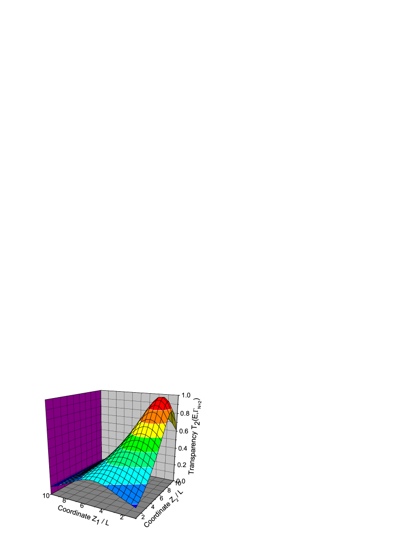
Figure 2: One example of the shape for the transparency $\mathcal{T}_{2}(E,\Gamma_{N=2})$ profile as the function of impurity positions $\mathcal{Z}_{1}$ and $\mathcal{Z}_{2}$. The distinctive maximum correspond to resonant configuration of type $(\mathrm{c})$, by classification scheme for two-impurity tunneling, when the energy of the incident particle $\epsilon\sim\exp(-\mathcal{L}/2)$. In the $x$ and $y$ axes is shown the ratio $\mathcal{Z}/\mathcal{L}$ in pixel such that 10 pixels correspond to ratio $\mathcal{Z}/\mathcal{L}=1$ and in the $z$ axis is shown absolute value of the tunnel probability.

C) General case of $N$ impurity centers arranged as $0<\mathcal{Z}_{1}<\ldots<\mathcal{Z}_{N}<\mathcal{L}$: in this case detailed analysis on the basis of above suggested formalism is very difficult, but rough estimation for the tunneling probability $\langle\mathcal{T}_{N}(E)\rangle$ may be found. It turns out that the picture of tunneling under conditions of large $N\gg 1$ breaks into effectively two-centers problem. This is true if among all centers there are two, which separated as $\delta\mathcal{Z}=\mathrm{max}\{\mathcal{Z}_{j+1}-\mathcal{Z}_{j}\}\sim|\ln|\epsilon||$. Such constraint comes from the fact that the $S_{11}=\epsilon e^{\delta\mathcal{Z}}$ matrix element of the scattering matrix is exponentially dominant and if in some energy interval we can put $S_{11}\sim 1$ than tunneling occur with maximum probability, otherwise it exponentially small. Subsequently, tunnelling via these centers dominate the whole tunneling process. The main contribution to the tunneling probability $\langle\mathcal{T}_{N}(E)\rangle$ in summation formula Eq. (27) comes form optimal $N$ such that $N=N_{\mathrm{opt}}\sim\sqrt{\mathcal{L}/|\ln c|}\gg 1$. The resonant impurity configuration, with mentioned constraint for $\delta\mathcal{Z}$, is in the order of $\Gamma^{\mathrm{res}}_{N}\sim 2^{-N}(N\delta\mathcal{Z}-\mathcal{L})^{N-1}/(N-1)!$ and asymptotic for the tunneling probability

$$\langle\mathcal{T}_{N}(E)\rangle\sim\exp\left(-2\sqrt{\mathcal{L}|\ln c|}-\mathcal{L}c-(\hbar\omega/T)\sqrt{\mathcal{L}/|\ln c|}\right).$$ (36)

To summarize, we have considered the tunneling of the quantum particle through disordered barrier in the regime of inelastic scattering when the tunneling probability is greater, compared to that of elastic scattering, in the out of resonance conditions. The energy interval $\triangle E$ where such situation may be realized is found and set of the tunneling probability functions $\mathcal{T}(E)$ for various impurity configurations presented.

References

- (1) I.M. Lifshitz, S.A. Gredeskul, L.A. Pastur, in Introduction to the theory of disordered systems, New York, ”Wiley”, (1988).
- (2) I.M. Lifshitz, V.Ya. Kirpichenkov, Sov. Phys. JETP 50(3), (1979)
- (3) M.E. Raikh, I.M. Ruzin, ”Mesoscopic Phenomena in Solids”, Edited by B.L. Altshuler, P.A. Lee and R.A. Webb, Elsevier Science Publishers B.V., (1991)
- (4) A.V. Chaplik, M.V. Entin, Sov. Phys. JETP, 40(3), (1974)
- (5) M.Ya. Azbel and P. Soven, Phys.Rev.B 27, p.831, (1983)
- (6) K.A. Matveev, A.I. Larkin, Phys.Rev.B 46(23), p.15337, (1992)
- (7) Jun Zang, Joseph L. Birman, Phys.Rev.B 47(16), p.10654, (1993)
- (8) V. Freilikher, M. Pustilnik, I. Yurkevich, Phys.Rev.B 53, p.7413, (1996)
- (9) C.W.J. Beenakker, Rev.Mod.Phys 69, p.731, (1997)
- (10) H. Willenberg, O. Wolst, R. Elpelt, W. Geisselbrecht, S. Malzer, and G. H. Döhler, Phys.Rev.B 65, p.035328, (2002)
- (11) R. Elpelt, O. Wolst, H. Willenberg, S. Malzer, and G. H. Döhler, Phys.Rev.B 69, p.205305, (2004)
- (12) R. Lake, G. Klimeck, S. Datta, Phys.Rev.B 47, p.6427, (1993)