Prediction of Ferromagnetic Correlations in Coupled Double-Level Quantum Dots

Abstract

Numerical results are presented for transport properties of two coupled double-level quantum dots. The results strongly suggest that under appropriate circumstances the dots develop a novel ferromagnetic correlation at quarter-filling (one electron per dot). In the strong coupling regime (Coulomb repulsion larger than electron hopping) and with the inter-dot tunneling larger than the tunneling to the leads, an S=1 Kondo resonance develops in the density of states, leading to a peak in the conductance. A qualitative “phase diagram”, incorporating the new FM phase, is presented. It is also shown that the conditions necessary for the ferromagnetic regime are less restrictive than naively believed, leading to its possible experimental observation in real quantum dots.

Strongly correlated electronic systems, such as high-T_c cuprates, heavy fermions, and manganites, display a variety of nontrivial collective states, which are difficult to analyze due to the many-body character of the interactions, and the difficulties in experimentally controlling the parameters determining these interactions. These problems are severe in materials that spontaneously grow in particular structures and patterns, with several effects (lattice, spin, charge, orbital) in direct competition. Therefore, the observation of a celebrated many-body effect, the Kondo effect, in a single quantum dot (QD) Goldhaber1 has captured the attention of the strongly correlated community. It is conceivable that the most interesting states that are spontaneously stabilized in some materials - and are very difficult to control - could instead be artificially created in a man-made structure. In this framework, a natural first-step is to analyze coupled QDs. In fact, the two-impurity Kondo problem - extensively studied since the 80’sjayap - can now be realized in a real system. Moreover, recent investigations have reported antiferromagnetic (AF) correlations between two single-level coupled QDs, in competition with Kondo correlations twoqd ; twoqdexp ; carlos1 . As a consequence, it is now clear that two of the most remarkable magnetic states known to exist in spontaneously grown materials - the Kondo and AF states - have already found realizations in the context of QDs. However, the other dominant magnetic state of some materials - the ferromagnetic (FM) state - has comparatively received much less attention craig . For the dream of artificially replicating collective states using QDs to be fulfilled, a realization of FM states must be achieved. The lack of attention to FM states in QDs should not be surprising in view of the physics of FM materials, such as manganites. Here, the FM state is reached by removing electrons (doping) from an AF state. Under the constraint of having one particle per level (1/2-filling), and only one level active per QD as in most previous investigations, the double-exchangezenner generated FM state cannot be realized. To reach a FM state, more levels need to be active, resulting in less than one electron per level.

In this Letter, clear evidence is presented for the development of ferromagnetic correlations between two double-level QDs multi1 : at 1/4-filling (one electron per dot), two coupled double-level QDs form a triplet state. Coupling this state to ideal metallic leads produces a Kondo resonance and a peak in the conductance. The results do not appear to be restricted to only a pair of QDs, but they seem valid for larger QD arrays. Basically here it is reported a realization of the double-exchange mechanism using QDs. Although the above mentioned effect is stronger if the appropriate intra-dot inter-level many-body interactions are added to the Hamiltonian, it is important to stress that these interactions are not necessary: considering just an intra-level Coulomb repulsion (Hubbard $U$) is enough to obtain qualitatively the same results, opening the possibility for the FM regime to be experimentally observable.

Figure 1: Schematic representation of the two double-level QDs system and the hopping amplitudes of Eqs. (1) and (3).

Figure 1 schematically depicts the system analyzed here and introduces the labelling for the different tunneling parameters $t^{\prime}$ and $t^{\prime\prime}$. To model this system, the impurity Anderson Hamiltonian that describes the two QDs with two levels (denoted $\alpha$ and $\beta$) is given by

$$H_{\rm d}=\sum_{i=1,2}\left\{\sum_{\sigma;\lambda=\alpha,\beta}Un_{i\lambda\sigma}n_{i\lambda\bar{\sigma}}+\sum_{\sigma\sigma^{\prime}}\left[U^{\prime}n_{i\alpha\sigma}n_{i\beta\sigma^{\prime}}-\right.\right.$$

$$\left.Jc^{\dagger}_{i\alpha\sigma}c_{i\alpha\sigma^{\prime}}c^{\dagger}_{i\beta\sigma^{\prime}}c_{i\beta\sigma}\right]+\sum_{\sigma}\left[V_{g}n_{i\alpha\sigma}+\right.$$

$$\left.\left.(V_{g}+\Delta V)n_{i\beta\sigma}\right]\right\}+\sum_{\sigma,\lambda=\alpha\beta}t^{\prime\prime}\left[c^{\dagger}_{1\lambda\sigma}c_{2\lambda\sigma}+\mbox{h.c.}\right],$$ (1)

where the first term represents the usual Coulomb repulsion between electrons in the same level (considered equal for both levels). The second term represents the Coulomb repulsion between electrons in different levels (the $U^{\prime}$ notation is borrowed from standard many-orbital studies in atomic physics). The third term represents the Hund coupling ($J>0$) that favors the alignment of spins and the fourth term is the energy of the states regulated by the gate voltage $V_{g}$. To decrease the number of free parameters, all the calculations presented here assume the following relations: $U^{\prime}=2U/3$ and $J=U-U^{\prime}$. As discussed later, the main result in this Letter does not depend on the specific values taken by $U^{\prime}$ and $J$. Note that $\alpha$ and $\beta$ are separated by $\Delta V$, and by modifying this parameter an interpolation between one- and two-level physics can be obtained. The last term represents the inter-dot coupling, with matrix element $t^{\prime\prime}$. For simplicity, we assume that there is no hopping between levels $\alpha$ and $\beta$. The dots are connected to the leads (represented by semi-infinite chains) by a hopping term with amplitude $t^{\prime}$, while $t=1$ is the hopping amplitude in the leads (and energy scale). More specifically,

$$H_{\rm leads} = t\sum_{i\sigma}\left[c_{li\sigma}^{\dagger}c_{li+1\sigma}+c_{ri\sigma}^{\dagger}c_{ri+1\sigma}+\mbox{h.c.}\right],$$ (2)

$$H_{\rm int} = t^{\prime}\sum_{\sigma,\lambda=\alpha,\beta}\left[c_{1\lambda\sigma}^{\dagger}c_{l0\sigma}+c_{2\lambda\sigma}^{\dagger}c_{r0\sigma}+\mbox{h.c.}\right],$$ (3)

where $c_{li\sigma}^{\dagger}$ ($c_{ri\sigma}^{\dagger}$ ) creates electrons at site $i$ with spin $\sigma$ in the left (right) contact. Site “0” is the first site at the left of the left dot and at the right of the right dot, for each half-chain. The total Hamiltonian is $H_{\rm T}=H_{\rm d}+H_{\rm leads}+H_{\rm int}$. Note that for $V_{g}$=$-U/2-U^{\prime}+J/2-\Delta V/2$, the Hamiltonian is particle-hole symmetric. Using the Keldysh formalism Meir-cnd , the conductance through this system can be written asnote1 $\sigma=\frac{e^{2}}{h}|t^{2}G_{lr}(E_{\rm F})|^{2}\left[\rho(E_{\rm F})\right]^{2}$. In practice, a cluster containing the interacting dots and a few sites of the leads is solved exactly, the Green functions are calculated, and the leads are incorporated through a Dyson Equation embedding procedure (details of the embedding have been provided elsewherecarlos1 ; interfere ). In Figs. 2-4, the cluster used involved the two QDs plus one lead site at left and right.

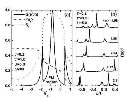
Figure 2: Results for the strong inter-dot tunneling regime ($t^{\prime\prime}/t^{\prime}\gg 1$) showing the presence of a ferromagnetic state at 1/4-filling and concomitant Kondo effect: (a) Conductance (solid line), charge occupancy per level and per spin (dashed line), and total spin $S_{\rm T}$ in the four levels of the dots (dotted line) vs. gate potential $V_{g}$ for two coupled double-level QDs. The values for the parameters are indicated. Note that the maximum in the conductance corresponds to a spin 1 Kondo peak that occurs when there is exactly one electron per dot and the total spin $S_{\rm T}\approx 1.0$. The other two peaks occur when there are 1 and 3 electrons in the two-dots system, corresponding to $S_{\rm T}=1/2$ Kondo resonances. (b) DOS indicating the presence of a Kondo resonance associated with the $S_{\rm T}=1$ Kondo peak in (a). The numbers on the right side indicate the total number of electrons inside the two quantum dots. $V_{g}$ takes the values $0.0$, $-0.5$, $-0.83$, $-1.12$, $-1.5$ from the top to the bottom curve. The Fermi level is located at $\omega/t=0.0$.

In Fig. 2a, results for conductance (solid line) at strong inter-dot tunneling ($t^{\prime\prime}/t^{\prime}\gg 1$) are shown. The main feature displayed is the peak at $V_{g}\approx-1.0$ (at and near 1/4-filling). The occupancy for this value of $V_{g}$ is approximately 1 electron per dot (dashed line $\times 4$) and the total spin $S_{\rm T}$ of the four levels note2 (dotted line) is $\approx 1.0$. The smooth charging of the levels as the gate potential decreases (in the peak region) indicates a possible Kondo regime. This is confirmed in Fig. 2b, where the density of states (DOS) close to the Fermi level is displayed as the gate potential varies from $0.0$ to $-1.5$ (top to bottom). Through this variation of $V_{g}$ the two dots are charged with one additional electron (the total mean charge varies from $\approx 1.6$ to $2.6$). One can clearly see a Kondo resonance pinned to the Fermi level. For lower values of the gate potential (in the region at and near 1/2-filling, with 2 electrons per dot) the conductance is drastically reduced and the total spin $S_{\rm T}$ inside the dots reaches its minimum value, indicating the formation of a global singlet state. Calculations of the total spin in each dot indicate that this singlet state is formed by the AF coupling of two spins $S=1$. A description of how this picture changes as the $t^{\prime\prime}$ decreases is shown in Fig. 3a, where results are shown for five different values of $t^{\prime\prime}$.

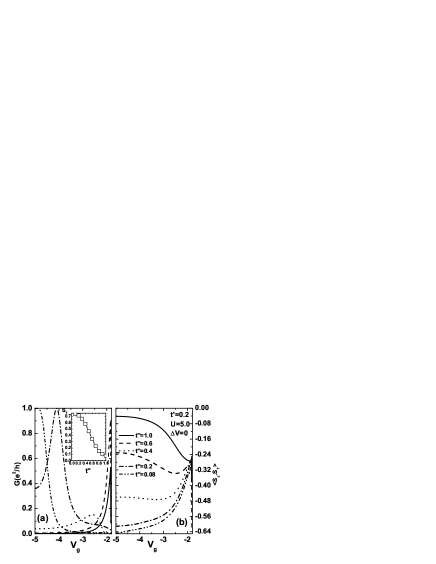
Figure 3: (a) Conductance $G$ vs. gate potential $V_{g}$ for different values of inter-dot tunneling ($t^{\prime\prime}=1.0,0.6,0.4,0.2,$ and $0.08$, see convention in (b)). $V_{g}$ varies across the region where the fourth electron is charged into the double-dot system. Note that the conductance at $V_{g}=-5.0$ gradually increases from zero (at strong tunneling, $t^{\prime\prime}=1.0$) to the maximum value (at weak tunneling, $t^{\prime\prime}=0.08$). This variation indicates a transition from two $S=1$ spins (in each dot) forming a global singlet to two uncorrelated $S=1$ spins, each forming a Kondo resonance with the lead conduction electrons. The inset shows the variation with $t^{\prime\prime}$ of the total spin inside the dots. (b) Variation with $t^{\prime\prime}$ of the spin-spin correlation between the total spin in the double-dot and a conduction electron located in the first site of the leads.

The conductance at the particle-hole symmetric point, $V_{g}=-5.0$, varies from zero, for $t^{\prime\prime}=1.0$, to 1.0 (in units of $e^{2}/h$), for $t^{\prime\prime}=0.08$. Fig. 3b shows how the Kondo correlation (between the total spin in the dots and a conduction electron in the first site of one of the leads) evolves from a negligible value for $t^{\prime\prime}/t^{\prime}\gg 1$ to a large value ($\approx-0.65$) for $t^{\prime\prime}/t^{\prime}<1$. The inset of Fig. 3a displays the change of the total spin (from $S_{\rm T}\approx 0.0$ to $\approx 3/4$) as $t^{\prime\prime}$ decreases. The two main peaks in the conductance discussed up to now were the $S_{\rm T}=1$ Kondo peak at 1/4-filling (relevant in the strong inter-dot tunneling regime) and the peak at 1/2-filling (relevant in the weak inter-dot tunneling regime). It is interesting to discuss how these peaks evolve as $\Delta V$ increases. Fig. 4a shows results for $t^{\prime\prime}/t^{\prime}\gg 1$ ($t^{\prime\prime}=1.0$, $U=5.0$ and $t^{\prime}=0.2$). The solid line displays the conductance and the doted line displays the total spin $S_{\rm T}$. Level separation $\Delta V$ increases from bottom to top (values for each graph are displayed in the left side). From $\Delta V=0.0$ up to $\Delta V\approx 0.6$ the width of the conductance peak slowly decreases, as also does the maximum value of $S_{\rm T}$. Above $\Delta V\approx 0.7$ (not shown) the narrowing of the peak accelerates (as does the decrease of $S_{\rm T}$), until the peak has all but vanished for $\Delta V=1.0$. For higher values of $\Delta V$ (top graph, $\Delta V=10.0$), the conductance shows the typical Coulomb blockade profile previously discussed carlos1 for coupled single-level dots when $t^{\prime\prime}/t^{\prime}\gg 1$.

Figure 4: Variation of the conductance with level separation $\Delta V$. The level separation is indicated for each curve. (a) $t^{\prime\prime}=1.0$: The gate potential decreases down to the particle-hole symmetric value, to highlight how the $S_{\rm T}=1$ Kondo peak varies with $\Delta V$. Note that all graphs have the same horizontal axis scale, except for the upper one (scale indicated on top). (b) $t^{\prime\prime}=0.08$: The gate potential varies down to the lowest value (total charging of the dots), to highlight the variation of the central peak (at the particle-hole symmetric point). Here also the upper graph has a different horizontal scale. A discussion of how the data interpolate between double- and single-level dots is given in the text.

Figure 4b shows the corresponding results for $t^{\prime\prime}/t^{\prime}<1$ ($t^{\prime\prime}=0.08$, $U=5.0$ and $t^{\prime}=0.2$). Note that the central peak does not change appreciably from $\Delta V=0.0$ to $\Delta V=2.0$. In fact, changes start only above $\Delta V=3.0$, when the central peak splits in two ($\Delta V\gtrsim 3.2$, not shown). For $\Delta V>3.4$ the two peaks start moving farther apart from each other and become very narrow. Finally, for $\Delta V=4.0$ the central peaks have disappeared, and the remaining structures are already similar to the single-level result $t^{\prime\prime}/t^{\prime}<1$. The top graph ($\Delta V=30.0$) is basically the result reported for single-level QDs at weak interdot tunneling carlos1 (if one discards the slight shoulders in the internal peaks).

Based on the results displayed on Fig. 4a, a qualitative phase diagram for the strong inter-dot tunneling regime can be sketched. In Fig. 5, the electron occupancy is in the horizontal axis (controlled by $V_{g}$) and $\Delta V$ is in the vertical axis. The left side (indicating 1/2-filling) is dominated by antiferromagnetism for all values of $\Delta V\lesssim U$. The singlet formed by the four levels is made of two spins $S\approx 1.0$. For $\Delta V>U$ one recovers the single-level picture. The right side of the phase diagram, which describes the evolution of the central peak in Fig. 4a, is more interesting. For $\Delta V<t^{\prime\prime}$ one has the novel FM region, where an $S_{\rm T}=1$ Kondo effect is present. For $\Delta V>t^{\prime\prime}$ an AF region is found, with no Kondo effect.

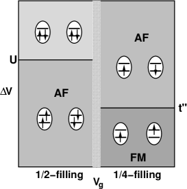
Figure 5: Qualitative phase diagram for the strong inter-dot tunneling regime ($t^{\prime\prime}/t^{\prime}\gg 1$). Horizontal axis indicates the level occupancy (controlled by $V_{g}$) and vertical axis indicates the level separation (controlled by $\Delta V$). In the 1/2-filling region, displayed in the left side, one goes from an AF coupling between two $S=1$ spins (for $\Delta V<V_{g}$) to a situation where the two lower levels are completely occupied (for $\Delta V>V_{g}$). In both cases there is no Kondo effect. On the other hand, in the 1/4-filling region (right side), for $\Delta V<t^{\prime\prime}$ one has the novel $S_{\rm T}=1$ FM Kondo region, which gives way to an AF region (with no Kondo effect) once $\Delta V>t^{\prime\prime}$. The regime with 3 electrons in the two dots is very narrow as a function of $V_{g}$ and it is not shown.

A finite size scaling analysis was done (results not shown) to verify how our numerical results converge with cluster sizefinite . The authors found out very little change in the results with increasing cluster size, giving us confidence that all the qualitative results here discussed are not caused by finite-size effects. It is also important to stress that the calculations presented in Fig. 2a were reproduced for $U^{\prime}=J=0.0$ (with the values of all other parameters kept the same as before ($U=5.0$, $t^{\prime\prime}=1.0$ and $t^{\prime}=0.2$)) and the results obtained barely changed. This indicates that the FM correlation and the $S_{\rm T}=1$ Kondo should be experimentally observable, since the only requirement is to have two double-level QDs with strong inter-dot tunnelingnote3 .

Figure 6 qualitatively summarizes the main result presented in this Letter: (a) For double-level coupled quantum dots in the strong inter-dot tunneling regime at 1/4-filling, FM correlations will develop and conductance through a Kondo channel is allowed. (b) On the other hand, single-level coupled QDs will develop AF correlations in the strong inter-dot tunneling regime and conductance is suppressed. The results discussed in this paper complete the analogy between QD states and magnetic phenomena in bulk materials. Previous investigations had shown that Kondo and AF states were possible in QDs. Now, at least theoretically, a regime with ferromagnetism has also been found, if more than one level per dot is active. Certainly, it would be important to confirm experimentally this prediction. Our calculations emphasizing multilevel dots present analogies with multi-orbital materials such as manganites, nickelates, cobaltites, and ruthenates. These compounds have a plethora of phases, all of which could find realizations in QDs systems as well.

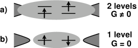
Figure 6: Schematic representation of the main result in this Letter

The authors acknowledge conversations with E. V. Anda and G. Chiappe. Support was provided by the NSF grants DMR-0122523 and 0303348.

References

- (1) D. Goldhaber-Gordon et al., Nature 391, 156 (1998).
- (2) C. Jayaprakash et al., Phys. Rev. Lett. 47, 737 (1981); K. Ingersent et al., Phys. Rev. Lett. 69, 2594 (1992).
- (3) A. Georges et al., Phys. Rev. Lett. 82, 3508 (1999); T. Aono et al., Phys. Rev. B 63, 125327 (2001); R. Lopez et al., Phys. Rev. Lett. 89, 136802 (2002); R. Aguado et al., Phys. Rev. B 67, 245307 (2003); M. N. Kiselev et al., Phys. Rev. B 68, 155323 (2003).
- (4) For experimental papers in double QDs, please see W. G. van der Wiel et al., Rev. Mod. Phys. 95, 1 (2003).
- (5) C. A. Büsser et al., Phys. Rev B 62, 9907 (2000).
- (6) N. J. Craig et al., Science 304, 565 (2004).
- (7) C. Zenner, Phys. Rev. 81, 440 (1951).
- (8) A. L. Yeyati et al., Phys. Rev. Lett. 83, 600 (1999); A. Silva et al., Phys. Rev. B 66, 195316 (2002); W. Hofstetter et al., Phys. Rev. Lett. 88, 016803 (2002); D. Boese et al., Phys. Rev. B 66, 125315 (2002); T-S. Kim et al., Phys. Rev. B 67, 235330 (2003).
- (9) Y. Meir et al., Phys. Rev. Lett. 66, 3048 (1991).
- (10) is the Green function that moves an electron from the left to the right lead, is the Fermi energy, and is the density of states of the leads: .
- (11) This method was originally proposed by E. V. Anda and G. Chiappe. See V. Ferrari et al. Phys. Rev. Lett. 82, 5088 (1999) and M.A. Davidovich et al., Phys. Rev. B 65 233310 (2002).
- (12) Note that the total spin in the four levels in the two quantum dots (denoted as and obtained through =, where , where labels the dots and labels the levels) is not a good quantum number (since the dots are not isolated). However, gives a good indication on the nature of the Kondo effect ( or ).
- (13) For a finite size scaling analysis of similar systems, see C. A. Büsser et al., to appear in Phys. Rev. B.
- (14) One can understand why an effective FM is generated (even in the absence of the Hund and the terms) by using the following argument: At 1/4-filling (two electrons in the four levels), the hopping from one lead to the adjacent dot (and vice-versa) is maximized when the spins of the electrons in the levels and in the same QD are parallel to each other. A strong inter-dot tunneling then generates an effective FM coupling between the QDs. Therefore, the only restriction for the FM coupling seems to be that the leads should have just one conduction channel.