Average path length in uncorrelated random networks with hidden variables

Abstract

Analytic solution for the average path length in a large class of uncorrelated random networks with hidden variables is found. We apply the approach to classical random graphs of Erdös and Rényi $(ER)$, evolving networks introduced by Barabási and Albert as well as random networks with asymptotic scale-free connectivity distributions characterized by an arbitrary scaling exponent $\alpha>2$. Our result for $2<\alpha<3$ shows that structural properties of asymptotic scale-free networks including numerous examples of real-world systems are even more intriguing then ultra-small world behavior noticed in pure scale-free structures and for large system sizes $N\rightarrow\infty$ there is a saturation effect for the average path length.

During the last few years random, evolving networks have become a very popular research domain among physicists 0a ; 0b ; BArev ; 2 . A lot of efforts were put into investigation of such systems, in order to recognize their structure and to analyze emerging complex properties. It was observed that despite network diversity, most of real web-like systems share three prominent structural features: small average path length ($APL$), high clustering and scale-free (SF) degree distribution 0a ; 0b ; BArev ; 2 ; 14 . Several network topology generators have been proposed to embody the fundamental characteristics BA1 ; 15 ; 12 ; krapPRL2001 ; krapPRE2001 ; 16 ; calPRL2002 .

To find out how the small-world property (i.e. small $APL$) arises, the idea of shortcuts has been proposed by Watts and Strogatz 32 . To understand where the ubiquity of scale-free distributions in real networks comes from, the concept of evolving networks basing on preferential attachment has been introduced by Barabási and Albert BA1 . Recently Calderelli and coworkers calPRL2002 have presented another mechanism that accounts for origins of power-law connectivity distributions. It is interesting that the mechanism is neither related to dynamical properties nor to preferential attachment. Caldarelli et al. have studied a simple static network model in which each vertex $i$ has assigned a tag $h_{i}$ (fitness, hidden variable) randomly drawn from a fixed probability distribution $\rho(h)$. In their fitness model, edges are assigned to pairs of vertices with a given connection probability $\widetilde{p}_{ij}$, depending on the values of the tags $h_{i}$ and $h_{j}$ assigned at the edge end points. Similar models have been also analyzed in several other studies gohPRL2001 ; chuComb2002 ; sodPRE2002 .

A generalization of the above-mentioned network models has been recently proposed by Boguñá and Pastor-Satorras bogPRE2003 . In the cited paper, the authors have argued that such diverse networks like classical random graphs of Erdös and Rényi $(ER)$, fitness model proposed by Caldarelli et al. and even scale-free evolving networks introduced by Barabási and Albert $(BA)$ may be described by a common formalism. Boguñá and Pastor-Satorras have derived analytical expressions for connectivity distributions $P(k)$ and relations describing degree correlations in such networks as functions of distributions of hidden variables $\rho(h)$ and the probability of an edge establishment $\widetilde{p}_{ij}$. In this paper we present an analytical description of main topological properties of the foregoing networks. We derive a general theoretical formalism describing metric features (i.e. $APL$, intervertex distance distribution) of random networks with hidden variables, assuming that the connection probability scales as $\widetilde{p}_{ij}\sim h_{i}h_{j}$ info1 . The last assumption concerning the factorised form of $\widetilde{p}_{ij}$ translates into the absence of two-point correlations and applies to a broad class of networks.

The issue of the small-world property is of great importance for network studies. The property directly affects such crucial fields like information processing in different communication systems (including the Internet) 26 ; havPRL1 ; havPRL2 ; 30 , disease or rumor transmission in social networks 33 ; 34 ; 35 as well as network designing and optimization 29 ; 31 ; 46 ; PRLoptimal . Not long ago, there was a strong belief that all the processes become more efficient when the mean distance between network sites is smaller. Recently however, it was shown that the small-world property may have an unfavorable influence on such phenomena like synchronizability PRLsynchro .

Despite the universality and usefulness of the small-world concept, except a few cases newPRL2000 ; szaPRE2002 ; havPRLultra ; dorNuc2003 , satisfactory calculations of the average path length ($APL$) almost do not exists. Even in the case of aged Erdös - Rényi graphs only a scaling relation (not an exact formula) describing $APL$ is known $l_{ER}\sim\ln N/\ln\langle k\rangle$ BArev . In this paper we derive an exact formula for the average distance $l_{ij}$ between any two nodes $i$ and $j$ characterized by given values of hidden variables $h_{i}$ and $h_{j}$. Averaging the quantity $l_{ij}$ over all pairs of vertices we obtain the average path length characterizing the whole network. It is important to stress that our formulas for $APL$ do not posses any free parameters, therefore may be directly compared with results of computer simulations. In this paper we have tested our analytic results against numerical calculations performed for Erdös - Rényi classical random graphs, $BA$ model and scale-free networks $P(k)\sim k^{-\alpha}$ with arbitrary scaling exponent $\alpha$. In all the cases we obtain a very good agreement between our theoretical predictions and results of numerical investigation.

Let us start with the following lemma.

Lemma 1

If $A_{1},A_{2},\dots,A_{n}$ are mutually independent events and their probabilities fulfill relations $\forall_{i}P(A_{i})\leq\varepsilon$ then

$$P(\bigcup_{i=1}^{n}A_{i})=1-\exp(-\sum_{i=1}^{n}P(A_{i}))-Q,$$ (1)

where $0\leq Q<\sum_{j=0}^{n+1}(n\varepsilon)^{j}/j!-(1+\varepsilon)^{n}$.

Proof. Using the method of inclusion and exclusion feller we get

$$P(\bigcup_{i=1}^{n}A_{i})=\sum_{j=1}^{n}(-1)^{j+1}S(j),$$ (2)

with

$$S(j)=\sum_{1\leq i_{1}<i_{2}<\dots<i_{j}\leq n}^{n}P(A_{i_{1}})P(A_{i_{2}})\dots P(A_{i_{j}})$$

$$=\frac{1}{j!}\left(\sum_{i=1}^{n}P(A_{i})\right)^{j}-Q_{j},$$ (3)

where $0\leq Q_{j}\leq\left(n^{j}/j!-\left({}^{n}_{j}\right)\right)\varepsilon^{j}$. The term in bracket represents the total number of redundant components occurring in the last line of (Average path length in uncorrelated random networks with hidden variables). Neglecting $Q_{j}$ it is easy to see that $(1-P(\cup A_{i}))$ corresponds to the first $(n+1)$ terms in the MacLaurin expansion of $\exp(-\sum P(A_{i}))$. The effect of higher-order terms in this expansion is smaller than $R<(n\varepsilon)^{n+1}/(n+1)!$. It follows that the total error of (1) may be estimated as $Q<\sum_{j=1}^{n}Q_{j}+R$. This completes the proof.

Let us notice that the terms $Q_{j}$ in (Average path length in uncorrelated random networks with hidden variables) disappear when one approximates multiple sums $\sum_{1\leq i_{1}<i_{2}<\dots<i_{j}\leq n}^{n}$ by corresponding multiple integrals. For $\varepsilon=A/n\ll 1$ the error of the above assessment is less then $A^{2}\exp(A)/n$ and may be dropped in the limit $n\rightarrow\infty$.

At the moment we briefly repeat (after Ref. bogPRE2003 ) the main properties of random networks with hidden variables and connection probability $\widetilde{p}_{ij}$ given by

$$\widetilde{p}_{ij}=\frac{h_{i}h_{j}}{\beta},$$ (4)

where $\beta$ is a certain constant. In the case of random networks, where two-point correlations at the level of hidden variables are absent we have

$$\beta=\langle h\rangle N,$$ (5)

whereas in correlated BA networks the prefactor gains another form. Boguñá and Pastor-Satorras have shown that degree distribution $P(k)$ in such uncorrelated networks is given by

$$P(k)=\sum_{h}\frac{e^{-h}h^{k}}{k!}\rho(h),$$ (6)

where $\rho(h)$ describes a distribution of hidden variables. The above relation between both distributions $P(k)$ and $\rho(h)$ implies a relation between their moments

$$\langle h^{n}\rangle=\langle k(k-1)\dots(h-n+1)\rangle,$$ (7)

and respectively

$$\langle h\rangle=\langle k\rangle,\;\;\;\;\;\;\;\langle h^{2}\rangle=\langle k(k-1)\rangle.$$ (8)

With respect to our following calculations the relation (6) requires a few comments. Firstly, let us note that for $k\rightarrow\infty$ the Poisson-like propagator, that accompanies the distribution $\rho(h)$ in the formula for $P(k)$, is a sharply peaked function analogous to delta $\delta_{h,k}$. For this reason, in the limit of large nodes degrees we obtain a correspondence between the studied uncorrelated networks with hidden variables and random graphs with a given degree sequence (the so-called configuration model) newPRE2001

$$P(k)\sim\rho(k).$$ (9)

Another very important conclusion that comes from considerations performed in Ref. bogPRE2003 and seems to affect our later derivations is that we can not generate uncorrelated random networks with power-law degree distribution $P(k)\sim k^{-\alpha}$ and the scaling exponent $2\leq\alpha<3$ by means of the factorised probability (4) (see also masPRE2003 ; parkPRE2003 ). The axiomatic definition of probability requires $\widetilde{p}_{ij}\leq 1$, giving the condition for the maximum value of the the hidden variable $h_{max}\sim\sqrt{N}$. When we think about hidden variables as about desired degrees (as sketched in the previous paragraph) the condition for $k_{max}\simeq h_{max}$ is in contradiction to the cut-off of the power-law degree distribution $k_{cut}\sim N^{1/(\alpha-1)}$ info2 that allows for nodes with degrees higher than $k_{max}$. For this reason, our formalism describing metric properties of random uncorrelated networks should not work well for SF networks with $2\leq\alpha<3$. In contrast to the above discussion, we noticed that our analytical predictions are consistent with numerical calculations performed for scale-free networks with arbitrary scaling exponent $\alpha>2$. We suspect that the unexpected conformity for networks with $2\leq\alpha<3$ may be related to the extreme small fraction of bad pairs of nodes with large degrees that do not fulfill the condition $\widetilde{p}_{ij}\leq 1$ (see Appendix A).

Now, we come back to the main subject of the paper, it means the issue of the average path length in random networks. Let us consider a walk of length $x$ crossing index-linked vertices $\{i,v_{1},v_{2}\dots v_{(x-1)},j\}$. Because of the lack of correlations the probability of such a walk is described by the product $\widetilde{p}_{iv_{1}}\>\widetilde{p}_{v_{1}v_{2}}\>\widetilde{p}_{v_{2}v_{3}}\dots\widetilde{p}_{v_{(x-1)}j}$, where $\widetilde{p}_{ij}$ gives a connection probability between vertices $i$ and $j$ (4). At this stage it is important to stress that the graph theory distinguishes a walk from a path 45 . A walk is just a sequence of vertices. The only condition for such a sequence is that two successive nodes must be the nearest neighbors. A walk is termed a path if all of its vertices are distinct. In fact, we are interested in the shortest paths. In order to do it, let us consider the situation when there exists at least one walk of the length $x$ between the vertices $i$ and $j$. If the walk(s) is(are) the shortest path(s) $i$ and $j$ are exactly $x$-th neighbors otherwise they are closer neighbors. In terms of statistical ensemble of random graphs krzPRE2001 the probability $p_{ij}(x)$ of at least one walk of the length $x$ between $i$ and $j$ expresses also the probability that these nodes are neighbors of order not higher than $x$. Thus, the probability that $i$ and $j$ are exactly $x$-th neighbors is given by the difference

$$p_{ij}^{*}(x)=p_{ij}(x)-p_{ij}(x-1).$$ (10)

In order to write the formula for $p_{ij}(x)$ we take advantage of the lemma (1)

$$p_{ij}(x)=1-\exp[-\sum_{v_{1}=1}^{N}\dots\sum_{v_{(x-1)}=1}^{N}\widetilde{p}_{iv_{1}}\dots\widetilde{p}_{v_{(x-1)}j}],\;\;\;$$ (11)

where $N$ is the total number of vertices in a network. A sequence of $(x+1)$ vertices $\{i,v_{1},v_{2}\dots,v_{(x-1)},j\}$ beginning with $i$ and ending with $j$ corresponds to a single event $A_{i}$ and the number of such events is given by $n=N^{x-1}$. Putting (4) into (11) and replacing the sum over nodes indexes by the sum over the hidden variable distribution $\rho(h)$ one gets

$$p_{ij}(x)=1-\exp\left[-\frac{h_{i}h_{j}}{\langle h^{2}\rangle N}\left(\frac{\langle h^{2}\rangle N}{\beta}\right)^{x\;}\right].$$ (12)

Due to (10) the probability that both vertices are exactly the $x$-th neighbors may be written as

$$p_{ij}^{*}(x)=F(x-1)-F(x),$$ (13)

where

$$F(x)=\exp\left[-\frac{h_{i}h_{j}}{\langle h^{2}\rangle N}\left(\frac{\langle h^{2}\rangle N}{\beta}\right)^{x\;}\right].$$ (14)

The above calculations require a few comments. First of all, note that the assumption underlying (1) is the mutual independence of all contributing events $A_{i}$. In fact, since the same edge may participate in several $x-$walks there exist correlations between these events. Nevertheless, it is easy to see that the fraction of correlated walks is negligible for short walks ($x\ll N$) that play the major role in random graphs showing small-world behavior. It is also important to stress that our formalism does not neglect loops.

Let us point out that having relations (13) and (14), describing the probability that the shortest distance between two arbitrary nodes $i$ and $j$ equals $x$, one can find almost all metric properties of studied networks afcond2 . For example, averaging (13) over all pairs of vertices one obtains the intervertex distance distribution $p(x)=\langle\langle p_{ij}^{*}(x)\rangle_{i}\rangle_{j}$. It is also possible to calculate $z_{x}$ - the mean number of vertices a certain distance $x$ away from a randomly chosen vertex $i$. The quantity can be written as $z_{x}=\int p_{ij}^{*}(x)\rho(h_{j})Ndh_{j}$. Note that taking only the first two terms of power series expansion of both exponential functions in (13) and making use of (4) and (8) one gets the relationship $z_{x}=z_{1}(z_{2}/z_{1})^{x-1}=\langle k\rangle(\langle k^{2}\rangle/\langle k\rangle-1)^{x-1}$ that was obtained by Newman et al. newPRE2001 when assuming a tree-like structure of random graphs with arbitrary degree distribution.

Taking advantage of (13) one can calculate the expectation value for the average distance between $i$ and $j$

$$l_{ij}(h_{i},h_{j})=\sum_{x=1}^{\infty}\>x\>p_{ij}^{*}(x)=\sum_{x=0}^{\infty}F(x).$$ (15)

Notice that a walk may cross the same node several times thus the largest possible walk length can be $x=\infty$. The Poisson summation formula allows us to simplify the above sum (see Appendix B)

$$l_{ij}(h_{i},h_{j})=\frac{-\ln h_{i}h_{j}+\ln N+\ln\langle h^{2}\rangle-\gamma}{\ln N+\ln\langle h^{2}\rangle-\ln\beta}+\frac{1}{2},$$ (16)

where $\gamma\simeq 0.5772$ is the Euler’s constant. The average intervertex distance for the whole network depends on a specified distribution of hidden variables $\rho(h)$

$$l=\frac{-2\langle\ln h\rangle+\ln N+\ln\langle h^{2}\rangle-\gamma}{\ln N+\ln\langle h^{2}\rangle-\ln\beta}+\frac{1}{2}.$$ (17)

We need to stress that both parameters $l_{ij}$ and $l$ diverge when the argument of the logarithmic function in the denominator of both expressions (16) and (17) approaches one i.e. $N\langle h^{2}\rangle/\beta=1$. Note, that substituting (5) for $\beta$ in the last condition and then taking advantage of (7) one recovers the well-known estimation for percolation threshold $\langle k^{2}\rangle/\langle k\rangle=2$ in undirected random networks with arbitrary degree distribution havPRL1 ; molloy1 ; calPRL2000 ; golPRE2003 (see Appendix C).

To test the formula (17) we start with the well-known networks: $ER$ classical random graphs, $BA$ model and scale-free networks. The choice of these networks is not accidental. The models play an important role in the network science. The $ER$ model was historically the first one but it has been realized it is too random to describe real networks. The most striking discrepancy between $ER$ model and real networks appears when comparing degree distributions. As mention at the beginning of the paper degree distributions follow a power-law in most of real systems, whereas classical random graphs exhibit Poisson degree distribution. It was found that the most generic mechanism driving real networks into scale-free structures is the linear preferential attachment. The simplest model that incorporates the rule of preferential attachment was introduced by Barabási and Albert BA1 . Other interesting mechanisms leading to scale-free networks were proposed by Goh et al. gohPRL2001 and Caldarelli et al. calPRL2002 . Goh and coworkers were the first who pointed out that power-law connectivity distribution $P(k)$ may result from the Zipf law applied to hidden variable distribution $\rho(h)\sim h^{-\alpha}$. The concept of the Zipf law has been next developed by Caldarelli et al. in their paper calPRL2002 . In fact, the most important achievement of the mention paper by Caldarelli et al. relates to a nontrivial discovery that scale-free networks may be also obtained from exponential distribution of fitnesses $\rho(h)\sim e^{-h}$. Since however, the case of scale-free networks with exponentially distributed fitnesses does not fulfill (4), we do not take it into account in this paper. In the present study, we examine the case of scale-free networks with underlying scale-free distributions of hidden variables.

Below we show that our formalism describing metric properties of random networks may be successfully applied to all the above listed network models.

Classical $ER$ random graphs. Note that the only way to recover the Poisson degree distribution form the expression (6) is to assume

$$\rho_{ER}(h)=\delta_{\langle k\rangle,h}.$$ (18)

Now, applying the distribution $\rho_{ER}(h)$ to (17) we get the formula for the average path length in classical random graphs

$$l_{ER}=\frac{\ln N-\gamma}{\ln\langle k\rangle}+\frac{1}{2}.$$ (19)

Until now only a rough estimation of the quantity has been known. One has expected that the mean intervertex distance of the whole ER graph scales with the number of nodes in the same way as the network diameter. We remind that the diameter $d$ of a graph is defined as the maximal shortest distance between any pair of vertices and $d_{ER}=\ln N/\ln\langle k\rangle$ BArev . Fig.1 shows the prediction of the equation (19) in comparison to the numerically calculated $APL$ in classical random graphs.

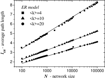
Figure 1: The average path length $l_{ER}$ versus network size $N$ in $ER$ classical random graphs with $\langle k\rangle=4,10,20$. The solid curves represent numerical prediction of Eq.(19).

Scale-free $BA$ networks. The basis of the $BA$ model is its construction procedure BA1 ; BA2 . Two important ingredients of the procedure are: the continuous network growth and the preferential attachment. The network starts to grow from an initial cluster of $m$ fully connected vertices. Each new node that is added to the network creates $m$ links that connect it to previously added nodes. The preferential attachment means that the probability of a new link growing out of a vertex $i$ and ending up in a vertex $j$ is given by

$$\widetilde{p}_{ij}^{BA}=m\frac{k_{j}(t_{i})}{\sum_{l}k_{l}(t_{i})},$$ (20)

where $k_{j}(t_{i})$ denotes the connectivity of a node $j$ at the time $t_{i}$, when a new node $i$ is added to the network. Taking into account the time evolution of nodes degree in $BA$ network (i.e. putting $k_{j}(t_{i})=m\sqrt{t_{i}/t_{j}}$), the probability of a link between $i$ and $j$ can be rewritten in the following form

$$\widetilde{p}_{ij}^{BA}=\frac{m}{2}\frac{1}{\sqrt{t_{i}t_{j}}},$$ (21)

that is equivalent to (4) when assuming $h_{i}=1/\sqrt{t_{i}}$, $h_{j}=1/\sqrt{t_{j}}$ and $\beta_{BA}=2/m$. The distribution of hidden variables $\rho_{BA}(h)$ in BA networks follows the relation

$$\rho_{BA}(h_{i})dh_{i}=\tilde{P}(t_{i})dt_{i},$$ (22)

where $\tilde{P}(t_{i})=1/N$ is the distribution of nodes attachment times $t_{i}$ for a network of size $N$. After a simple algebra one gets

$$\rho_{BA}(h)=\frac{2}{N}h^{-3},$$ (23)

for $h=1/\sqrt{N},\dots,1$. Now, it is simple to calculate the average distance (16) between any two nodes in BA networks

$$l_{ij}^{BA}(h_{i},h_{j})=\frac{-\ln(h_{i}h_{j})-\ln(m/2)-\gamma}{\ln\ln N+\ln(m/2)}+\frac{3}{2}.$$ (24)

Averaging (24) over all pairs of vertices one obtains $APL$ characterizing the whole network

$$l_{BA}=\frac{\ln N-\ln(m/2)-1-\gamma}{\ln\ln N+\ln(m/2)}+\frac{3}{2}.$$ (25)

Fig.2 shows the $APL$ in $BA$ networks as a function of the network size $N$ compared with the analytical formula (25). There is a visible discrepancy between the theory and numerical results when $\langle k\rangle=2m=4$. The discrepancy disappears when the network becomes denser i.e. when $\langle k\rangle$ increases. The same effect will appear at Fig.4, letting us deduce that for some reasons our formalism works better for denser networks.

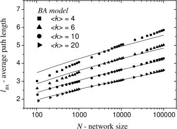
Figure 2: Characteristic path length $l_{BA}$ versus network size $N$ in $BA$ networks. Solid lines represent Eq.(25).

Scale-free networks with arbitrary scaling exponent. Let us start with the well-known model of scale-free networks introduced by Goh et al. (Model $A$) gohPRL2001 and its certain modification proposed by Caldarelli et al. (Model $B$) calPRL2002 . We show that both models $A$ and $B$ possess peculiar properties that make application of our theoretical approach impossible. Next, we make use of a general procedure described at the beginning of the paper to generate uncorrelated networks with asymptotic power-law connectivity distributions (Model $C$).

Model $A$. To construct the network one has to perform the following steps: (i.) prepare a fixed number $N$ of vertices; (ii.) assign fitness (hidden variable) $h_{i}=i^{-\tau}$, with $0\leq\tau<1$, to every node $i=1,\dots,N$; (iii.) select two vertices $i$ and $j$ with probabilities equal to normalized hidden variables, $h_{i}/(\langle h\rangle N)$ and $h_{j}/(\langle h\rangle N)$, respectively, and add an edge between them unless one already exists; (iv.) repeat previous steps until $mN$ edges are made in the system. Goh and coworkers have showed that the resulting network generated in accordance with the above procedure exhibits asymptotic power-law degree distribution

$$P(k)\sim k^{-\alpha},$$ (26)

where

$$\alpha=1+1/\tau,$$ (27)

that gives $2<\alpha<\infty$. Although in these networks probability of a connection approximately factorizes (4)

$$\widetilde{p}_{ij}^{A}=1-\left(1-\frac{h_{i}h{j}}{(\langle h\rangle N)^{2}}\right)^{mN}\simeq\frac{h_{i}h_{j}}{\beta_{A}},$$ (28)

where $\beta_{A}=\langle h\rangle^{2}N/m$, there is one important feature of the model. The non-analytic statement, included in the step (iii.) of the construction procedure expressed as add an edge unless one already exists, gives rise to uncontrolled intervertex correlations both for large $m$ and small $\alpha<3$.

Model $B$. Caldarelli and coworkers have modified the original model introduced by Goh et al. by assigning to nodes random fitnesses $h_{i}$ taken from a given distribution $\rho(h)\sim h^{-\alpha}$, instead of deterministic values $h_{i}=i^{-\tau}$. They also assumed a modified edge establishment process: for every pair of vertices $i$ and $j$ a link was drawn with probability (4), where $\beta_{B}=(h_{max})^{2}$. Although the foregoing value of $\beta_{B}$ assures us of $\widetilde{p}_{ij}^{B}<1$, it is strongly overestimated and makes resulting networks very sparse with a large content of isolated nodes info3 .

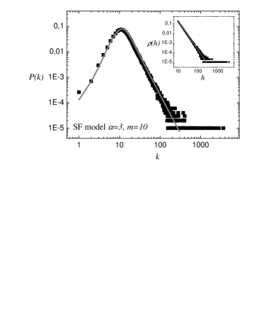
Figure 3: Model C. Degree distribution $P(k)$ (the main layer) for random network with underlying hidden variable distribution given by a power-law (the inset). Scatter data represent results of numerical calculations, whereas solid curves express formulas (6) and (29), respectively for $P(k)$ and $\rho(h)$.

Model $C$. In order to avoid features incorporated in both models $A$ and $B$, we have generated networks possessing asymptotic scale-free behavior for $k\gg 1$ coming out of power-law distributions of hidden variables

$$\rho(h)=\frac{(\alpha-1)m^{(\alpha-1)}}{h^{\alpha}},$$ (29)

for $h=m,\dots,h_{max}$, where $h_{max}\simeq mN^{1/(\alpha-1)}$ (see info2 ) and connection probability given by (4) and (5). A typical behavior of connectivity distribution $P(k)$ for networks generated in accordance with this procedure is presented at Fig.3. Note that for $k>m$ the connectivity distribution is well described by the power law $P(k)\sim k^{-\alpha}$ (9).

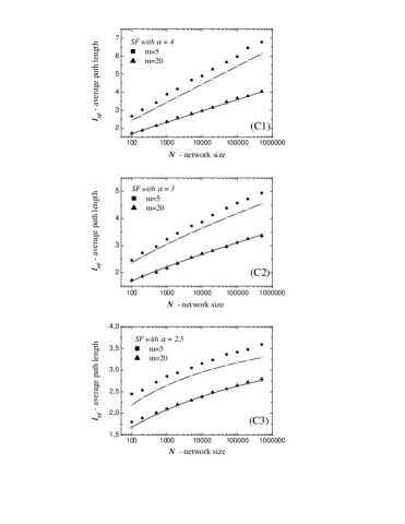
Figure 4: Model C. The average path length versus network size $N$ for $\alpha=4$ (C1), $\alpha=3$ (C2) and $\alpha=2.5$ (C3). The scatter data represent numerical calculations. Solid curves with open squares in the case of $m=5$ (open circles in the case of $m=20$) express analytical predictions of Eqs. (30), (31) and (32) respectively for (C1),(C2) and (C3).

Applying the distribution (29) to the formula (17) one obtains

• for $\alpha>3$

  $$l^{\alpha>3}=\frac{\ln N+\ln(\frac{\alpha-1}{\alpha-3})-\frac{2}{\alpha-1}-\gamma}{\ln(\frac{\alpha-2}{\alpha-3})+\ln m}+\frac{1}{2},$$ (30)

• for $\alpha=3$

  $$l^{\alpha=3}=\frac{\ln N-\ln(\frac{m}{2})-1-\gamma}{\ln\ln N+\ln(\frac{m}{2})}+\frac{3}{2},$$ (31)

• for $2<\alpha<3$

  $$l^{\alpha<3}=\frac{(\frac{2}{\alpha-1})\ln N+\ln(\frac{\alpha-1}{3-\alpha})-(\frac{2}{\alpha-1})-\gamma}{(\frac{3-\alpha}{\alpha-1})\ln N+\ln(\frac{\alpha-2}{3-\alpha})+\ln m}+\frac{1}{2}.$$ (32)

Fig.4 shows predictions of the above equations in comparison with numerically calculated shortest paths. We would like to stress that regardless of the value of $\alpha$, for denser networks (with higher values of parameter $m$), one can observe an excellent agreement between our theory and numerical results.

Summarizing, depending on the value of scaling exponent $\alpha$ one can distinguish three scaling regions for the average path length in scale-free networks. In the limit of large systems $N\to\infty$, $APL$ scales with network size according to relations

• for $\alpha>3$

  $$l^{\alpha>3}\sim\ln N,$$ (33)

• for $\alpha=3$

  $$l^{\alpha=3}\sim\frac{\ln N}{\ln\ln N},$$ (34)

• for $2<\alpha<3$

  $$l^{\alpha<3}=\frac{2}{3-\alpha}+\frac{1}{2}.$$ (35)

Note that although the results for $\alpha\geq 3$ are consistent with estimations obtained by other authors havPRLultra ; dorNuc2003 , the case of $2<\alpha<3$ is different. In opposite to previous estimations signaling the double logarithmic dependence $l^{\alpha<3}\sim\ln\ln N$, our calculations for the same range of $\alpha$ predict that there is a saturation effect for the mean path length in large networks. Since the assumption underlying estimations leading to double logarithmic dependence in $APL$ was a pure scale-free behavior of degree distribution, we suspect that this discrepancy may result from ambiguous behavior of $P(k)$ in our model. Let us note that in our model $C$ there is a relatively small number of nodes with small degrees $k$ (see Fig.3). Since distances between such nodes are usually very large in comparison to distanced between nodes with higher degrees, thus their absence may lead to the domination of the $APL$ parameter by distances between the population of nodes characterized by medium degrees. Our result shows that for $2<\alpha<3$ structural properties of asymptotic scale-free networks including numerous examples of real-world networks may be even more intriguing then ultra-small world behavior reported for pure scale-free systems.

To conclude, in this paper we have presented theoretical approach for metric properties of uncorrelated random networks with hidden variables. We have derived a formula for probability $p^{*}_{ij}(x)$ (13) that the shortest distance between two arbitrary nodes $i$ and $j$ equals $x$. We have shown that given $p^{*}_{ij}(x)$ one can find every structural characteristic of the studied networks. In particular, we have applied our approach to calculate exact expression for the average path length (17) in such networks. We have shown that our formalism may be successfully applied to such diverse networks like classical random graphs of Erdös and Rényi, evolving networks introduced by Barabási and Albert as well as random networks with asymptotic scale-free connectivity distributions characterized by arbitrary scaling exponent $\alpha>2$. In all the studied cases we noticed a very good agreement between our theoretical predictions and results of numerical investigation.

Acknowledgments. First of all, we wish to thank to anonymous Referee for critical comments which helped us to refine our paper. In the preliminary version of the paper afcond1 we have used a node degree notation, that was not accurate enough with reference to the analyzed problem. Following the comments given by the anonymous Referee we have reformulated our approach in a language of hidden variables. We are also thankful to Sergei Dorogovtsev for his critical comments to an earlier draft of this paper. One of us (AF) acknowledge The State Committee for Scientific Research in Poland for support under grant No. $2P03B01323$.

Appendix A. The condition $\widetilde{p}_{ij}\leq 1$ (4) is not fulfilled for pairs of vertices $i$ and $j$ possessing large hidden variables (or desired degrees) $h_{i}$ and $h_{j}$. To justify our calculations, we have to assure ourselves that the fraction of such pairs is very small

$$\int_{h_{min}}^{h_{max}}\rho(h_{j})\int_{\widetilde{p}_{ij}\beta/h_{j}}^{h_{max}}\rho(h_{i})dh_{i}dh_{j}\ll 1.$$ (36)

Using the Chebyshev’s inequality feller and solving (36) with respect to $\widetilde{p}_{ij}\leq 1$ one gets

$$\frac{\langle h^{2}\rangle}{\langle h\rangle^{2}}(\langle h^{2}\rangle-\langle h\rangle^{2})\ll N^{2},$$ (37)

where we assumed $\beta=\langle h\rangle N$. It can be shown that every network that is considered in this paper fulfill the condition.

Appendix B. The Poisson summation formula states

$$\sum_{x=0}^{\infty}F(x)=\frac{1}{2}F(0)+\;\;\;\;\;\;\;\;\;\;\;\;\;\;\;\;\;\;\;\;\;\;\;\;\;\;\;\;\;\;\;\;\;\;\;\;\;\;\;\;\;\;\;\;\;\;\;\;\;\;\;\;\;\;$$ (38)

$$\;\;\;\;\;\;\;\;\;\;\;\;\;\;\;\int_{0}^{\infty}F(x)dx+2\sum_{n=1}^{\infty}\left(\int_{0}^{\infty}F(x)\cos(2n\pi x)dx\right).$$

Applying the formula to (15)

$$l_{ij}(h_{i}h_{j})=\sum_{x=0}^{\infty}\exp\left[-\frac{h_{i}h_{j}}{\langle h^{2}\rangle N}\left(\frac{\langle h^{2}\rangle N}{\beta}\right)^{x\;}\right]$$ (39)

one realizes that in most of cases

$$\frac{h_{i}h_{j}}{\langle h^{2}\rangle N}\simeq 0$$ (40)

that gives $F(0)=1$. One can also find that

$$\int_{0}^{\infty}F(x)dx=-Ei\left(-\frac{h_{i}h_{j}}{\langle h^{2}\rangle N}\right)/\ln\left(\frac{\langle h^{2}\rangle N}{\beta}\right),$$ (41)

where $Ei(y)$ is the exponential integral function that for negative arguments is given by $Ei(-y)=\gamma+\ln y$ ryzyk , where $\gamma\simeq 0.5772$ is the Euler’s constant. Finally, it is easy to see that owing to the generalized mean value theorem every integral in the last term of the summation formula (38) is equal to zero. It follows that the equation for the APL between $i$ and $j$ is given by (16).

Appendix C. Note that, using additional assumptions one can simply reformulate both formulas (16) and (17) as well as the whole formalism in terms of node’s degrees instead of hidden variables. For more details see afcond1 .

References

- (1) S.Bornholdt and H.G.Schuster, Handbook of Graphs and networks, Wiley-Vch (2002).
- (2) S.N. Dorogovtsev and J.F.F.Mendes, Evolution of Networks, Oxford Univ.Press (2003).
- (3) R.Albert and A.L.Barabási, Rev. Mod. Phys. 74 47 (2002).
- (4) S.N.Dorogovtshev and J.F.F.Mendes, Adv.Phys. 51 1079 (2002).
- (5) S.H.Strogatz, Nature 410 268 (2001).
- (6) A.L.Barabási and R.Albert, Science 286, 509 (1999).
- (7) R.Albert and A.L.Barabási, Phys. Rev. Lett. 85 5234 (2000).
- (8) S.N.Dorogovtsev et al., Phys. Rev. Lett. 85 4633 (2000).
- (9) P.L.Krapivsky et al., Phys. Rev. Lett. 86 5401 (2001).
- (10) P.L. Krapivsky and S. Redner, Phys. Rev. E 63 066123 (2001).
- (11) K.Klemm and V.M.Eguíluz, Phys. Rev. E 65 036123 (2002).
- (12) G. Caldarelli et al., Phys. Rev. Lett. 89, 258702 (2002).
- (13) D.J.Watts and S.H.Strogatz, Nature 393 440 (1998).
- (14) K.-I. Goh et al., Phys. Rev. Lett. 87, 278701 (2001).
- (15) F. Chung and L. Lu, Annals of Combinatorics 6, 125 (2002).
- (16) B. Söderberg, Phys. Rev. E 66, 066121 (2002).
- (17) M. Boguñá and R. Pastor-Satorras, Phys. Rev. E 68, 036112 (2003).
- (18) In fact, all the derivations presented in this paper may be simply reformulated when assume a general factorised form of , where and denote arbitrary functions.
- (19) R.Albert et al., Nature 406, 378 (2000).
- (20) R. Cohen et al., Phys. Rev. Lett. 85, 4626 (2000).
- (21) R. Cohen et al., Phys. Rev. Lett. 86, 3682 (2001).
- (22) R.Pastor-Satorras et al., Phys. Rev. Lett 87 258701 (2001).
- (23) V.M.Eguíluz and K.Klemm, Phys. Rev. Lett. 89 108701 (2002).
- (24) R.Pastor-Satorras and A.Vespignani, Phys. Rev. Lett. 86 3200 (2001).
- (25) Z.Dezső and A.L.Barabási, Phys. Rev. E 65 055103 (2002).
- (26) L.A.Adamic et al., Phys. Rev. E 64 046135 (2001).
- (27) B.J.Kim et al., Phys. Rev. E 65 027103 (2002).
- (28) S.Valverde et al., cond-mat/0204344 (2002).
- (29) L.A. Braunstein et al., Phys. Rev. Lett. 91 168701 (2003).
- (30) T. Nishikawa et al., Phys. Rev. Lett. 91 014101 (2003).
- (31) M.E.J. Newman et al., Phys. Rev. Lett. 84, 3201 (2000).
- (32) G. Szabó et al., Phys. Rev. E 66, 026101 (2002).
- (33) R. Cohen and S. Havlin, Phys. Rev. Lett. 90 058701 (2003).
- (34) S.N. Dorogovtsev et al., Nucl. Phys. B 653, 307 (2003).
- (35) W.Feller, An Introduction to Probability Theory and its Applications, John Wiley and Sons (1968).
- (36) M.E.J. Newman et al., Phys. Rev. E 64, 026118 (2001).
- (37) S. Maslow et al., cond-mat/0205379.
- (38) J. Park and M.E.J. Newman, Phys. Rev. E 68, 026112 (2003).
- (39) In a finite network, the cut-off of degree distribution may be estimated from yielding .
- (40) R.J.Wilson, Intr. to Graph Theory, Longman (1985).
- (41) Z. Burda et al., Phys. Rev. E 64, 046118 (2001).
- (42) A. Fronczak et al., How to calculate the main characteristics of random graphs - a new approach, cond-mat/0308629.
- (43) M. Molloy and B. Reed, Ran. Struct. and Algor. 6, 161 (1995).
- (44) D.S. Callaway et al., Phys. Rev. Lett. 85 5468 (2002).
- (45) A.V. Goltsev et al., Phys. Rev. E 67 026123 (2003).
- (46) A.L.Barabási et al., Physica A 272 173 (1999).
- (47) We have numerically checked that in the case of scaling exponents and network size (see Fig.2 in calPRL2002 ) the amount of isolated vertices approaches .
- (48) A. Fronczak et al., Average path lenght in random networks, cond-mat/0212230.
- (49) I.S. Gradshteyn et al., Table of Integrals, Series, and Products, Academic Press (2000).