Temperature dependence of the tunneling amplitude between Quantum Hall edges

Abstract

Recent experiments have studied the tunneling current between the edges of a fractional quantum Hall liquid as a function of temperature and voltage. The results of the experiment are puzzling because at “high” temperature ($600-900$ mK) the behavior of the tunneling conductance is consistent with the theory of tunneling between chiral Luttinger liquids, but at low temperature it strongly deviates from that prediction dropping to zero with decreasing temperature. In this paper we suggest a possible explanation of this behavior in terms of the strong temperature dependence of the tunneling amplitude.

In the last twenty years quantum Hall systems have been a rich source of information about the physics of correlated electron systems. One example is the edge of a Fractional quantum Hall system which represents one of the best realization of a strictly one dimensional interacting system. Indeed, Wen showed that the low-energy density excitations localized along the edges of a fractional quantum Hall liquid are effectively described by a chiral Luttinger Liquid ($\chi$LL) Wen (1990, 1991), with the effective interaction parameter given by the bulk filling factor $\nu_{b}$.

Tunneling experiments offer an effective way to probe in detail the predictions of the $\chi$LL model Wen (1991); Kane and Fisher (1992); D’Agosta et al. (2003). In particular, measurements of the tunneling current from an external metallic gate into the edge of a 2DEG have beautifully confirmed the theoretical prediction of a tunneling current proportional to $V_{T}^{\frac{1}{\nu_{b}}}$ for $k_{B}T\ll eV_{T}$ ($V_{T}$ being the potential difference between the edge and the gate) Milliken et al. (1995); Chang et al. (1996); Grayson et al. (1998). The tunneling of fractionally charged quasiparticles between the edges of a fractional quantum Hall liquid has also been studied experimentally by several groups Chung et al. (2003a, b); Roddaro et al. (2003). Of particular interest to us are the recent measurements performed in the weak tunneling regime at $\nu_{b}=1/3$ by Roddaro et al. Roddaro et al. (2003). According to the theory, one expects that, in this experiment, the tunneling current must scale as $V_{T}^{2\nu_{b}-2}$ for $k_{B}T\ll eV_{T}$ and be linear in $V_{T}$ for $V_{T}\ll k_{B}T$. The zero-bias tunneling conductance, $\left.\frac{dI_{T}}{dV_{T}}\right|_{V_{T}=0}$, furthermore, should grow as $T^{2\nu_{b}-2}$ with decreasing temperature Wen (1991); Kane and Fisher (1992); D’Agosta et al. (2003). Contrary to this expectation, while in the temperature range $600$ mK $<T<900$ mK one observes a growing conductance with decreasing temperature, below $600$ mK one sees a dramatic drop in the tunneling conductance. We emphasize that this is in glaring contrast not only with the prediction of the weak tunneling theory, but also with the exact theory Fendley et al. (1995) valid in both weak- and strong-tunneling regimes.

In this Letter we argue that these puzzling data may be explained by a strong temperature dependence of the inter-edge tunneling amplitude. More precisely, we will show that the spatial separation between the edges of a fractional quantum Hall liquid increases with decreasing temperature, resulting in a rapid loss of overlap between the edges and a consequent collapse of the tunneling amplitude on a temperature scale $T_{0}$ quite comparable to the $600$ mK observed in the experiment.

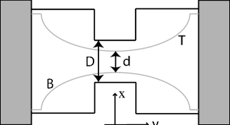
Figure 1: Simple scheme of the experimental setup. The current is carried by the quasi-particle in the edge states that are forced to stay close by the presence of the geometrical constriction of width $D$. Note that, inside the constriction, the edges are at the distance $d$ with $d\ll D$. We assumed as the $0$ for the $y$ coordinate the position where the edge distance is minimal and the tunneling takes place (see Ref. D’Agosta et al., 2003 for further details on the choice of the reference frame and Ref. Roddaro et al., 2003 for the details about the actual device).

The common starting point for calculating the differential tunneling conductance is a model consisting of two $\chi$LL s (the two edges) coupled by the tunneling hamiltonian

$$H_{T}=\Gamma\hat{\Psi}^{\dagger}_{T}(0)\hat{\Psi}_{B}(0)+\Gamma^{*}\hat{\Psi}^{\dagger}_{B}(0)\hat{\Psi}_{T}(0)$$ (1)

where $\Gamma$ is a phenomenological tunneling amplitude and the operators $\hat{\Psi}_{T(B)}(0)$ destroy a quasiparticle of fractional charge $e^{*}=\nu_{b}e$ at a point “$0$” in the top or bottom edge respectively (see Fig. 1). A standard perturbative calculation leads to the following expression for the differential tunneling conductance $G=\frac{dI_{T}}{dV_{T}}$ at $V_{T}=0$Wen (1991); D’Agosta et al. (2003):

$$G=\frac{e^{2}}{h}\left(\frac{\Gamma}{\hbar v}\right)^{2}\left(\frac{k_{B}T}{\hbar\omega_{0}}\right)^{2\nu_{b}-2}B(\nu_{b},\nu_{b})$$ (2)

where $v$ is the velocity of the edge modes, $\omega_{0}$ is an ultraviolet frequency cutoff related to the microscopic cutoff length $a$ by $\omega_{0}=\frac{v}{a}$, and $B(x,y)$ is the Euler beta function Abramowitz and Stegun (1964).

It is normally assumed that the tunneling amplitude is independent of temperature: if this were true it would imply $G\propto T^{2\nu_{b}-2}$, increasing with decreasing temperature. However, an analysis of the experimental data of Ref. Roddaro et al., 2003, shows that the situation is quite different. We extract the value of $\Gamma$ from the measured values of the conductance simply by inverting Eq. (2), using $v\simeq 4\times 10^{5}~{}\mathrm{m/s}$ for the edge wave velocity Aleiner and Glazman (1994) and $a=100~{}\mathrm{\AA}$ Wen (1991) for the ultraviolet length cutoff. The values of $\Gamma$ obtained in this manner are shown as solid dots in Fig. 2. Notice that $\Gamma$ increases rapidly with temperature below about $600$ mK and more slowly for $T>600$ mK.

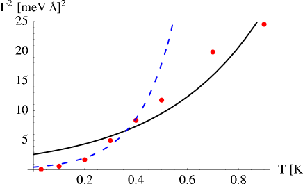
Figure 2: The variation of $|\Gamma|^{2}$ with temperature. The points (red) are the experimental results Roddaro et al. (2003) obtained from the the evaluation of Eq. (2). The lines are two fits with the function $g\exp(T/T_{0})$. The solid line (black) is a fit with all the experimental data and gives $g=2.6~{}(\mathrm{meV\AA})^{2}$ and $T_{0}=400$ mK while for the dashed line (blue) we have considered only temperatures below $400$ mK and gives the estimates $g=0.5~{}(\mathrm{meV\AA})^{2}$ and $T_{0}=140$ mK.

To understand this unexpected behavior, we begin by recalling that the tunneling amplitude arises from the overlap of single particle states localized in front of each other on the top and bottom edges. For two coherent states in the lowest Landau level centered respectively at $0,T$ and $0,B$ (see Fig. 1) the matrix element of the noninteracting hamiltonian is (up to an irrelevant phase factor)

$$\Gamma=\frac{\hbar^{2}}{2m^{*}\ell}e^{-\frac{d^{2}}{4\ell^{2}}}$$ (3)

where $d$ is the distance between the edges at the center of the constriction, $\ell$ is the magnetic length, and $m^{*}$ is the effective mass. It is important to realize that $d$ is typically much smaller than the geometric separation, $D$, between the split gates (in the experiments of Ref. Roddaro et al. (2003), with $m^{*}\simeq 0.067m$ for GaAs, and $\ell\simeq 100~{}\mathrm{\AA}$, one has $d\sim 3-5\ell$ , while $D\sim 30\ell$) and that its value is determined by equilibrium considerations discussed in detail below. Due to the exponential dependence of $\Gamma$ on $d$ even a relatively small variation of $d$ with temperature can have a large effect on $\Gamma$. Moreover we will show that, at low temperatures, $d$ varies linearly with the temperature.

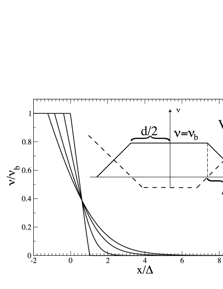
Figure 3: The solution of Eq. (6) for various temperatures $k_{B}T/U=0.01,~{}0.51,~{}0.81,~{}1.01$). Inset: Plot of of the local filling factor profile at $T=0$ (solid line) and of the confining potential (dashed line).

Our picture of the system in shown in the inset of Fig. 3. The center of the Hall bar is occupied by an incompressible quantum Hall strip of width $d$, sandwiched between two compressible regions of smoothly varying density. Since the density tapers off from the uniform value in the incompressible strip to zero over a distance of several magnetic lengths, what we are showing here is essentially the situation depicted by Chklovskii et al. in their classical electrostatic theory of edge channels Chklovskii et al. (1992, 1993). The density profile is determined, at $T=0$, by minimizing the sum of the electrostatic energy and the confinement energy, subject to the constraint of having an incompressible strip at the center of the system . In order to arrive at an analytically tractable model we assume that the system is translationally invariant in the $y$ direction (i.e., the density profile depends only on $x$) and that the electron-electron interaction is screened, due to the presence of the split gates, beyond a characteristic screening length $\lambda$, also of the order of several magnetic lengths. We also assume that the system is symmetric with respect to $x=0$ and study below only the part with $x>0$: thus we neglect any interaction between the top and the bottom part of the system. None of these simplifications alters the qualitative features of the solution.

The total energy associated with a given density profile $n(x)$ can be written as

$$E=\frac{\pi e^{2}\lambda L}{\epsilon_{b}}\int n(x)^{2}~{}dx+L\int V(x)n(x)~{}dx$$ (4)

where $\epsilon_{b}$ is the dielectric constant, $V(x)$ is the external confining potential (from gates, etc.), and $L$ is the length of the system in the $y$ direction. The integral runs over the top inhomogeneous region. At finite temperature, we also need to include the electronic entropy. This is obtained in the standard way from the assumption that the local filling factor $\nu(x)\equiv 2\pi\ell^{2}n(x)$ gives the probability of a single particle state centered at $x$ in the lowest Landau level to be occupied. Thus, we have

$$\begin{split}S=-\frac{k_{B}L}{2\pi\ell^{2}}\int&\left\{\nu(x)\ln\nu(x)\right.\\ &\left.+[1-\nu(x)]\ln[1-\nu(x)]\right\}~{}dx.\end{split}$$ (5)

The edge density profile is now computed from the requirement that the free energy $F=E-TS$ is stationary with respect to small variations of the density, subject to the constraint of global particle number conservation and with the further condition $\nu(x)=\nu_{b}$ at the edge of the incompressible strip (notice that the position of this edge is itself to be determined). These requirements easily lead to the equation

$$U\nu(x)+V(x)+k_{B}T\ln\left[\frac{\nu(x)}{1-\nu(x)}\right]=\mu$$ (6)

which must be satisfied in the compressible region determined by the conditions $0<\nu(x)<\nu_{b}$. Here $U=\lambda e^{2}/\epsilon_{b}\ell^{2}$ represents a typical interaction energy, $\mu$ is the chemical potential, which fixes the total particle number, and the edge of the incompressible strip occurs at the position for which $\nu(x=d(T)/2)=\nu_{b}$ (cf. Fig. 3). For the sake of simplicity we take the position of the edge at $T=0$ as the origin of the coordinate, $x\to x-d(0)/2$. To proceed, we assume that around this point the external potential can be linearly expanded, $V(x)=e{\cal E}x$, where ${\cal E}$ is the electric field. Eq. (6) admits an elegant solution in this case. However, we expect that non-linear terms yield no qualitative differences as long as one considers not too high temperatures. To begin with, by setting $T=0$, we easily find the zero-temperature solution

$$\nu_{0}(x)=\left\{\begin{array}[]{lc}\nu_{b}\left(1-\frac{x}{\Delta}\right),&0<x<\Delta\\ \nu_{b},&x<0\\ 0,&x>\Delta\end{array}\right.$$ (7)

where $\Delta=\frac{U}{e{\cal E}}\nu_{b}$ is the width of the compressible region and $\mu=U\nu_{b}$.

At finite temperature, the chemical potential must be chosen in such a way that the total particle number remains the same as at $T=0$: therefore we must have

$$\int_{x_{0}}^{\infty}\nu(x)~{}dx=\int_{x_{0}}^{\Delta}\nu_{0}(x)~{}dx=-\nu_{b}x_{0}+\frac{\Delta\nu_{b}}{2},$$ (8)

where the position of the edge, $x_{0}$, is determined by the condition $\nu(x_{0})=\nu_{b}$. Due to the linearity of the external potential, the integral on the left hand side of Eq. (8) can be evaluated analytically by a change of variable from $x$ to $\nu$ after an integration by parts. This yields

$$\begin{split}\int_{x_{0}}^{\infty}\nu(x)~{}dx=&-\nu_{b}x_{0}-\frac{\Delta\nu_{b}}{2}+\frac{1}{e\mathcal{E}}\left\{\mu\nu_{b}\right.\\ &\left.-k_{B}T[\nu_{b}\ln\nu_{b}+(1-\nu_{b})\ln(1-\nu_{b})]\right\}.\end{split}$$ (9)

By comparing Eq. (8) and Eq. (9) we get the temperature shift of the chemical potential

$$\mu(T)-\mu(0)=\frac{k_{B}T}{\nu_{b}}\left[\nu_{b}\ln\nu_{b}+(1-\nu_{b})\ln(1-\nu_{b})\right]$$ (10)

and by evaluating Eq. (6) for $x=x_{0}$, we have

$$x_{0}=\frac{k_{B}T}{U}\frac{\ln(1-\nu_{b})}{\nu_{b}^{2}}\Delta$$ (11)

which yields the effective edge separation by recalling that $d(T)=d(0)+2x_{0}$. Fig. 3 shows the numerical solution of Eq. (6) for $\nu(x)$ obtained for different temperatures. Notice that the edge of the incompressible strip shifts inward as predicted by Eq. (11).

Putting Eq. (11) in Eq. (3) we finally arrive at

$$|\Gamma(T)|^{2}=|\Gamma(0)|^{2}e^{T/T_{0}}$$ (12)

where

$$k_{B}T_{0}=\left|\frac{\nu_{b}}{\ln(1-\nu_{b})}\right|\frac{\lambda}{2\Delta}\left(\frac{\nu_{b}e^{2}}{\epsilon_{b}d}\right)~{}.$$ (13)

From the experiments Roddaro et al. (2003) we estimate that $\Delta\simeq 3\lambda$ and $d(0)\simeq 4\ell$: thus we obtain $T_{0}\simeq 600~{}\mathrm{mK}$ which is comparable with the value obtained from the fits shown in Fig. 2. Since $\Delta=U\nu_{b}/e{\mathcal{E}}$, one expects that the characteristic temperature scale $T_{0}$ increases by making the confining potential steeper. This prediction appears to be qualitatively in agreement with recent experiments Roddaro et al. (2004) where the behavior of the tunneling conductance has been investigated as a function of the gate voltage controlling the quantum point contact. For sufficiently negative gate voltage the tunneling conductance is consistent with the prediction of the $\chi$LL model with a constant $\Gamma$. This in turn is consistent with a large characteristic temperature scale $T_{0}$ as predicted by Eq. (13).

We believe that our electrostatic model, in spite of its simplicity, captures the essential aspects of the observed temperature dependence of the tunneling amplitude. The main effect of the temperature is to remove particles from the incompressible strip transferring them into the zone that was depleted at $T=0$. This causes a linear increase in entropy, coming primarily from the population of states that were initially empty. Let us emphasize that Eq. (5) takes into account only the entropy of the compressible strip and that the electrons in the incompressible strip are locked in a collective state of essentially zero entropy for temperatures below the fractional quantum Hall gap. Thus we do not expect that the general scenario presented here will be significantly affected by introducing more realistic features in the calculation of the energy and of the confining potential.

On the other hand, our analysis of the experiment assumes the validity of Eq. (2), itself a consequence of the weak tunneling theory of Wen. Recently, there have been suggestions that Eq. (2) might be invalidated by additional interactions between electrons on the same edge, since these interactions appear to change the scaling dimension of the tunneling Papa and MacDonald (2004). For that mechanism to be effective the long range intra-edge interaction must be stronger than the inter-edge interaction: this condition is unlikely to be satisfied in the present experimental setup.

As a final point, we note that the dependence of the inter-edge separation on temperature is not expected to translate into a dependence of this quantity on the applied voltage. Indeed, in the present experiment this voltage is just the Hall voltage created by the dc current injected in the Hall bar Roddaro et al. (2003). The effect of this current is to create different quasi-particle populations on the two edges. However, in our model, this will cause a rigid shift of both edges in the same direction thus leaving the distance between them and hence the tunneling amplitude unaffected.

In conclusion, in this Letter we have addressed the problem of determining the temperature dependence of the tunneling amplitude in the tunneling process between the edges of a fractional quantum Hall liquid. We have shown that the temperature modifies in a non trivial way the equilibrium distance between the edges, and therefore the tunneling amplitude which is a very sensitive function of the temperature.