Theory of Non-Coherent Spin Pumps

Abstract

We study electron pumps in the absence of interference effects paying attention to the spin degree of freedom. Electron-electron exchange interactions combined with a variation of external parameters, such as magnetic field and gate potentials, affect the compressibility-spin-tensor whose components determine the non-coherent parts of the charge and spin pumped currents. An appropriate choice of the trajectory in the parameter space generates an arbitrary ratio of spin to charge pumped currents. After showing that the addition of dephasing leads to a full quantum coherent system diminishes the interference contribution, but leaves the non-coherent (classical) contribution intact, we apply the theory of the classical term for several examples. We show that when exchange interactions are included one can construct a source of pure spin current, with a constant magnetic field and a periodic variation of gate potentials only. We discuss the possibility to observe it experimentally in GaAs heterostructures.

I Introduction

A pump is a very common device, it appears in many shapes and types, in physical systems as well as biological systems. A pump converts a periodic variation of the parameters that control it into a direct current. For example, in an Archimedes (or Auger) screw pump after one revolution “buckets” of water are lifted up, while the blades of the screw return to their position at the initial stage of the revolution. Rorres (2000)

As modern electronic devices, including electron pumps, become smaller and get into the mesoscopic size of a few nanometer to a fraction of micrometer, we need to consider also the wavy, i.e., quantum mechanical, nature of the electrons. Similar to the classical devices, a quantum pump converts periodic variations of its parameters at frequency $\omega$ into a DC current. Thouless (1983)

In both quantum and classical devices the pumping rate is proportional to the liquid pumped in one turn of the pump and to the revolution rate $\omega$. When the Archimedean screw is rotated too fast, turbulence and sloshing prevents the buckets from being filled and the pump stops to operate. Similarly, in small electronic devices, the pumping rate is proportional to $\omega$ only in the adiabatic limit — when $\omega$ is small enough.

While pumps exist for both interacting coherent quantum systems and interacting classical systems, the main theoretical studies of mesoscopic pumps were concentrated on the wavy nature of the electrons describing the pumps in terms of non-interacting coherent-scattering theory.Spivak95 ; Brouwer98 ; Avron02 ; Entin02 Several works discuss the effect of dephasing Moskalets and Buttiker (2001); Cremers and Brouwer (2001); Brouwer et al. (2002) which smears the wavy nature of electrons, suppresses interference effects and renders the system non-coherent, i.e., classical. The complexity of the full quantum problem in presence of interactionsJauho et al. (1994) allowed its study only in few examples of open quantum dots Aleiner and Andreev (1998) and Luttinger liquid.Sharma and Chamon (2001)

On the other hand, the early experimental studies of quantum-dot-turnstile pump Kouwenhoven et al. (1991); Pothier et al. (1991) are described in classical terms of interacting systems, namely, capacitance and oscillating “resistances” of tunnel barriers. In a more recent experiment, Switkes et al. (1999) coherent pumping was observed. (However, parasitical rectification effects may be relevant.Brouwer (2001); Rec )

In this manuscript we study the classical non-coherent effect of pumping and in particular we show how this classical effect directly emerges out of the quantum mechanical formulationBrouwer98 when dephasing sources exist. While the quantum-scattering description may include physics related to the spin degree of freedom,Sharma and Brouwer (2003) it treats electron-electron interaction on the Hartree level only. In this manuscript we include both direct and exchange interaction within the framework of a classical theory. This enables us to suggest a scheme to build a pure “spin battery” (see Sec. V.3) which is a key concept in the field of spintronics.

The remainder of the paper is organized as follows: in Sec. II we derive an expression for the non-coherent contribution for small electron pumps using a classical model that neglects interference effects completely. The formulation of pumps in classical terms allows us to include rather easily the effects of interactions between the electrons.

To describe effects of dephasing in a controlled manner Moskalets and Buttiker (2001); Cremers and Brouwer (2001) we include in Sec. III, following Ref. Moskalets and Buttiker, 2001, the effect of additional voltage leads on the (non-interacting adiabatic) quantum scattering theory of pumps. Spivak95 ; Brouwer98 ; Avron02 ; Entin02 We show that when the coupling to the dephasing leads is tuned properly to cause complete dephasing, the Brouwer formula, Brouwer98 which relates the pumping current to the scattering matrix and its time derivatives, reduces to the classical expressions developed in Sec. II. We compare the magnitudes of the quantum and classical contributions and study under what conditions the classical contribution dominates.

After constructing and justifying the classical theory of non-coherent pumps, we generalize it in Sec. IV to deal with spinfull electrons endowing our result with a topological interpretation. Finally, in Sec. V we deal with a possible realization of spin pumps in two dimensional electron gas of GaAs heterostructures. We show that under rather general conditions the spin current (similar to the Einstein‘s DC conductance formula) is given in terms of the thermodynamic density of states tensor of the system (the compressibility tensor). In the presence of a constant magnetic field, we find an appropriate trajectory in the parameter space such that a pure spin current will flow. This effect vanishes in the absence of exchange interaction.

In appendix A we discuss the relation between the classical non-coherent pumped current and the biased current, generated by rectification effects.Rec In appendix B we explore the relation between our theory and the theory of non-linear response. In this manuscript we do not include effects of charge discreteness leaving this for a future study.Sela and Oreg

II Classical Description of non-coherent Pumps

Consider the electrical circuit depicted in Fig. 1. Its purpose is to charge the capacitor $C$ from left and then to discharge it to the right, thus producing a net current from left to right without a bias voltage. The gate voltage, $V_{g}$, periodically charges and discharges the capacitor while the resistors, $R_{L}$ and $R_{R}$, control the direction of the charging and discharging processes.

To analyze the system it is convenient to define an asymmetry parameter

$$\alpha(R_{L},R_{R})=\frac{1}{2}\frac{R_{R}-R_{L}}{R_{R}+R_{L}}$$ (1)

running between $1/2$ for $R_{R}\gg R_{L}$ and $-1/2$ for $R_{R}\ll R_{L}$.

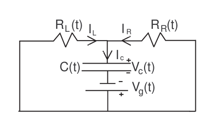
Figure 1: Equivalent circuit of a classical pump. A typical pumping cycle occurs when we charge the capacitor through the left resistor (keeping $R_{R}\gg R_{L}$) and discharge it through the right resistor (when $R_{R}\ll R_{L}$). In that case a net DC current flows in the clockwise direction in the large current loop.

The pumping circuit is operational even at a constant gate voltage, when $V_{g}=V_{0}$. Suppose that the capacitor may be typified by a parallel plate capacitor with a tunable area $A$, separation $d$ and permittivity $\varepsilon$. Initially the capacitor is at equilibrium with charge $Q_{0}=CV_{0}=\frac{\varepsilon AV_{0}}{2\pi d}$. Then its area is varied to $A^{\prime}=A-\delta A$ while $\alpha\approx-1/2\;(R_{R}\ll R_{L})$. As a result a charge $\delta Q_{0}$ will leave the capacitor to the right until equilibrium is restored. Then by changing the area back from $A^{\prime}$ to $A$ when $\alpha\approx 1/2$, we will pull the same amount of charge $\delta Q_{0}$ into the capacitor from the left. Repeating this process with a period $\tau$ will result in an average pumped current $\delta CV_{0}/\tau$ flowing from left to right.Rec  (A periodic variation of $d$ or $\varepsilon$ will have a similar effect.)

Proceeding formally, let $Q(t)$ be the instantaneous charge on the capacitor. The charge leaving the capacitor during a small time interval $dt$ is $-dQ(t)=-\dot{Q}(t)dt$. From current conservation and Kirchhoff‘s rules:

$$I_{L}+I_{R}=\dot{Q}(t)\equiv I_{c},\qquad I_{L}R_{L}=I_{R}R_{R},$$ (2)

the fraction of this out going charge, $-dQ(t)$, leaving via $R_{L}$ or via $R_{R}$ is

$$dQ_{R(L)}(t)=-\frac{R_{L(R)}}{R_{L}+R_{R}}dQ(t).$$ (3)

We define the pumped current as $I=\frac{\langle I_{L}\rangle-\langle I_{R}\rangle}{2}$ where $\langle O\rangle=\tau^{-1}\int_{0}^{\tau}O(t)dt$ denotes average over a period. Then $I$ may be expressed in terms of $Q(t)$ as

$$I=\frac{1}{\tau}\int_{0}^{\tau}dt\frac{1}{2}(I_{L}-I_{R})=\frac{1}{\tau}\int_{0}^{\tau}dt\alpha(t)\dot{Q}(t).$$ (4)

The charge $Q(t)$ should be determined by the equations of motion of the system which are governed by a Lagrangian $\cal{L}$, including a source term in the Euler-Lagrange equations which introduces dissipation:

$$\frac{\delta{\cal{L}}(Q,\dot{Q})}{\delta Q}-\frac{d}{dt}\frac{\delta{\cal{L}}(Q,\dot{Q})}{\delta\dot{Q}}=R\dot{Q},$$ (5)

where $R=R_{L}\parallel R_{R}=R_{L}R_{R}/(R_{L}+R_{R})$.

If the parameters, $x(t),y(t),\dots$, that control $Q$ and $\alpha$ in Eq. (4) are varied slow enough then $Q$ and $\alpha$ are functions of the instantaneous value of these parameters, and do not depend explicitly on time:

$$Q(t) = Q\left[x(t),y(t),\dots\right],$$

$$\alpha(t) = \alpha\left[x(t),y(t),\dots\right].$$ (6)

The parameters $x(t),y(t),\dots$ can be for example $V_{g},d,A,\varepsilon,R_{L},R_{R}$ or any combination of them, e.g., $\alpha$ itself. We will refer to this slow limit as the adiabatic limit. For each case that we study we will check how large should be the period $\tau$ for the adiabatic limit to be established. Roughly, the adiabatic condition is established when $\tau$ is larger than the effective $RC$ time of the circuit.

If there are only two parameters, then in the adiabatic limit the pumped current is

$$I=\frac{1}{\tau}\int_{0}^{\tau}dt\alpha[x(t),y(t)]\dot{Q}[x(t),y(t)].$$ (7)

Using now

$$\frac{dQ}{dt}=\frac{\partial Q}{\partial x}\frac{dx}{dt}+\frac{\partial Q}{\partial y}\frac{dy}{dt},$$

the current can be rewritten as a line integral along a trajectory ${\mathbb{L}}$ in the parameter space (see Fig. 2):

$$I=\frac{1}{\tau}\oint_{{\mathbb{L}}}(\alpha\partial_{x}Q,\alpha\partial_{y}Q)\cdot(dx,dy).$$ (8)

Because the parameters are varied periodically in time the trajectory is closed. Using Stoke’s theorem, the line integral can be transformed into a surface integral on the closed surface $\mathbb{S}$ bounded by the trajectory ${\mathbb{L}}$,

$$I = \frac{1}{\tau}\int\!\!\!\!\int_{\mathbb{S}}dxdyB^{\rm{eff}}=\frac{\phi^{\rm eff}}{\tau},$$

$$\nabla\times A^{\rm eff} = B^{\rm{eff}}=\partial_{x}\alpha\partial_{y}Q-\partial_{y}\alpha\partial_{x}Q=\nabla\alpha\times\nabla Q,$$

$$A^{\rm eff} = \alpha\nabla Q\text{ or }\frac{1}{2}\left(\alpha\nabla Q-Q\nabla\alpha\right),$$ (9)

where $B^{\rm{eff}}$ is an effective magnetic field in parameter space. The last ambiguity in the definition of $A^{\rm eff}$ is a result of a gauge freedom: an addition of the gradient term $\frac{1}{2}\nabla(\alpha Q)$ does not change $B^{\rm eff}$.

Equation (II) suggests that the charge pumped per cycle, $\tau I$, is equal to the flux of the effective magnetic field through the loop in parameter space $\phi^{\rm eff}$, as depicted in Fig. 2. Similar topological formulation for the pumped current was discussed in the quantum case Brouwer98 ; Avron02 while here we obtained a similar structure for the classical situation.

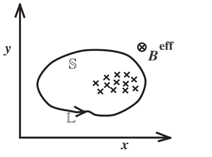
Figure 2: The pumped charge per period is the flux of an effective magnetic field inside the parameters trajectory.

II.1 Example: $x=\alpha$, $y=V_{g}$

Since no current is pumped if the asymmetry parameter $\alpha$ is kept fixed, we consider the simplest example where $\alpha$ itself is a pumping parameter. Substituting the Lagrangian of the circuit depicted in Fig. 1 (generalized to the case where the capacitance depends on its charge or on the voltage across it):

$${\cal{L}}(Q,\dot{Q})=-E_{c}(Q)+QV_{g},$$

$$E_{c}(Q)=\int_{0}^{Q}dQ^{\prime}V_{c}(Q^{\prime}),$$

$$V_{c}(Q)=\int_{0}^{Q}\frac{dQ^{\prime}}{C(Q^{\prime})}$$ (10)

in Eq. (5), one gets the equation of motion $V_{g}-V_{c}(Q)=\dot{Q}R$. Using $C=dQ/dV_{c}$ we get

$$V_{g}-V_{c}=RC\dot{V}_{c}.$$ (11)

The meaning of the adiabatic limit is clear in this equation. The typical time scale for changes in $V_{c}$ is the period time $\tau$. Therefore if $RC\ll\tau$ we can neglect the right hand side of the equation and establish the adiabatic limit $V_{c}(t)=V_{g}(t)$. Substituting this into Eq. (II) one gets

$$I=\frac{1}{\tau}\int\!\!\!\!\int_{\mathbb{S}}C(V_{g})d\alpha dV_{g},$$ (12)

so that $C$ plays the role of the effective magnetic field.

For $C=10^{-15}F$ at a frequency $\tau^{-1}=1GHz$ and with a gate voltage oscillations of $1mV$ the maximal pumped current is $1nA$.

II.2 Application to a more general electrical circuit

Consider the electrical circuit shown in Fig. 3 that generalizes the circuit depicted in Fig. 1. The analysis of the two circuits is similar: let us assume that we change the charge on capacitor $C_{m_{0}}$ by $dQ_{m_{0}}$ (by changing $V_{g~{}m_{0}}$), while keeping the charge on the other capacitors constant. Using Kirchhoff’s rules one can show that the fraction of $dQ_{m_{0}}$ flowing to the left via $R_{1}$, $dQ_{L}$, or to the right via $R_{N}$, $dQ_{R}$, is:

$$dQ_{R(L)}(t)=-\frac{R_{m_{0}}^{L(R)}}{\sum_{m=1}^{N}R_{m}}dQ_{m_{0}}(t),$$ (13)

where $R^{L}_{m_{0}}=\sum_{m=1}^{m_{0}}R_{m}$ and $R^{R}_{m_{0}}=\sum_{m=m_{0}+1}^{N}R_{m}$ are the resistances to the left and to the right of capacitor $C_{m_{0}}$ respectively.

The superposition principle generalizes Eq. (13) to

$$dQ_{R(L)}(t)=-\frac{\sum_{k}R_{k}^{L(R)}dQ_{k}(t)}{\sum_{m=1}^{N}R_{m}}$$ (14)

for any variation of $\{V_{g~{}k}\}$. Similarly, Eq. (12) which holds in the adiabatic limit becomes

$$I=\frac{1}{\tau}\int\!\!\!\!\int_{\mathbb{S}}\sum_{k=1}^{N-1}C(V_{g~{}k})d\alpha_{k}dV_{g~{}k},$$ (15)

where $\alpha_{k}=\frac{1}{2}\frac{R^{R}_{k}-R^{L}_{k}}{R^{R}_{k}+R^{L}_{k}}$.

In the next section we will show that a small quantum system subjected to dephasing can be described by the circuit depicted in Fig. 3.

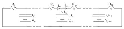
Figure 3: Generalization of the circuit in Fig. 1.

III Connection with Quantum Pumps subjected to Dephasing

The scattering approach for pumpsBrouwer98 relates the DC current flowing through a time dependent scatterer with its scattering matrix and with the time derivatives of the scattering matrix. However, in real physical systems there are processes that lead to uncertainty in the phase of the single electron; for example interaction with phonons and interaction between the electrons mediated by the electromagnetic environment. This effect is called dephasing. It is expected that a classical description will gradually take place as the dephasing becomes stronger.

To study the effect of dephasing on the quantum coherent pump in a controllable way we introduce dephasing leads Buttiker (1986); Brouwer et al. (2002) and show that in the limit of strong dephasing the pumping current approaches the classical limit given in Eq. (15). The effect of dephasing can be described in different ways which differ in details, but this variety of ways does not alter the main conclusion that a quantum system with strong dephasing can be described by a classical theory.

Consider a conducting wire subjected to a gate potential $V_{g}(r)$, $r\in[0,L]$, as shown in Fig. 4(a). To introduce dephasing in a controlled way we connect $N-1$ wave splitters of 4 legs Foo at the points $r=i\ell$, $i={1,2,...,N-1}$ along the wire, as shown in Fig. 4(b) (for $N=3$). The length $\ell$ determines the dephasing length of the model together with the wave splitter parameter $\epsilon$, as we will explain later. The wave splitters are described by the scattering matrix

$$\textbf{S}_{\rm{splitter}}(\epsilon)=\left(\begin{array}[]{cccc}0&\sqrt{1-\epsilon}&\sqrt{\epsilon}&0\\ \sqrt{1-\epsilon}&0&0&\sqrt{\epsilon}\\ \sqrt{\epsilon}&0&0&-\sqrt{1-\epsilon}\\ 0&\sqrt{\epsilon}&-\sqrt{1-\epsilon}&0\\ \end{array}\right),$$

where the third and forth lines and columns of the matrix correspond to the two legs of the reservoir that serves as a dephasor. Each wave splitter $i$ is connected to a reservoir $i$ held at voltage $V_{i}$. To mimic a dephasor that influences only the phase coherence of the waves in the sample and does not influence the total current, we tune the voltages $\{V_{i}\}$ so that no net charge flows into any of the reservoirs. In our time dependent problem we will assume that such conditions hold at all times.

(In a similar model of dephasing Das et al. (2003) one introduces an extra phase $\phi$ in selected points, which is averaged out after squaring the desired amplitude. The approach that we use differs from the later in the following way: the introduction of the reservoirs is accompanied by the addition of contact resistances, which renders the total resistance from left to right higher.)

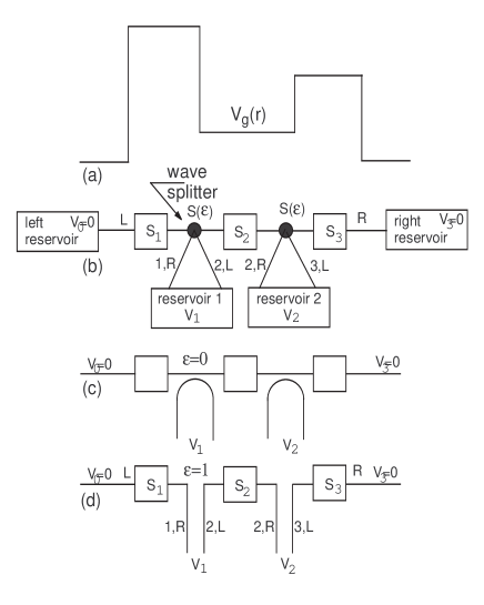
Figure 4: (a) The gate potential along the original quantum system without dephasing. (b) Introduction of dephasors, controlled by a parameter $\epsilon$. (c) $\epsilon=0$: The system is totaly coherent. (d) $\epsilon=1$: This configuration doesn’t allow any interference effects between different scatterers $S_{m}$.

For general $\epsilon$ the whole system, including the dephasing leads, is described by a S matrix of rank $2N$. The current in each lead is composed of two contributions, the pumped current (Brouwer formula Brouwer98 ) and the biased current (Landauer-Buttiker-Imry conductance formula Landauer (1957)). The voltages $\{V_{i}\}$ produce biased currents which cancel the pumped currents in each reservoir.

In the limit $\epsilon\rightarrow 0$ (without dephaing) the S matrix is block diagonal: it is a direct sum of $N$ rank $2$ matrices. One of them connects between the left and right reservoirs and describes scattering from the potential $V_{g}(r)$ between $r=0$ and $r=L$. The other matrices trivially connect each reservoir only to itself, i.e., the reservoirs are not connected to the wire, see Fig. 4(c).

In the limit $\epsilon\rightarrow 1$ we again have $\textbf{S}=\oplus_{m=1}^{N}\textbf{S}_{m}$. Now $\textbf{S}_{m}$ describes a potential barrier $V_{g(m)}(r)$ between two dephasors given by

$$V_{g(m)}(r)=\left\{\begin{array}[]{ll}V_{g}(r)&\textrm{$(m-1)\ell<r<m\ell$}\\ 0&\textrm{else}\end{array}\right..$$ (16)

The original barrier is split into $N$ sections, see Fig. 4(d). Notice that while the phase coherence between different sections is lost, they are correlated by the requirement for zero current in the reservoirs. The dephasing length is thus equal to $\ell$.

Let us concentrate on the $\epsilon=1$ case which is easier to handle, (mentioning that, in principle the model could be solved for any $\epsilon$) and parameterize the unitary scattering matrix of each section as

$$\textbf{S}_{m}=e^{i\Lambda_{m}}\left(\begin{array}[]{cc}e^{i\eta_{m}}\cos\theta_{m}&ie^{-i\phi_{m}}\sin\theta_{m}\\ ie^{i\phi_{m}}\sin\theta_{m}&e^{-i\eta_{m}}\cos\theta_{m}\\ \end{array}\right).$$ (17)

For this parametrization the Brouwer formula reads Avron02

$$2\pi/e\;dQ_{m,L}=-d\Lambda_{m}-\cos^{2}\theta_{m}d\eta_{m}+\sin^{2}\theta_{m}d\phi_{m}$$

$$2\pi/e\;dQ_{m,R}=-d\Lambda_{m}+\cos^{2}\theta_{m}d\eta_{m}-\sin^{2}\theta_{m}d\phi_{m},$$ (18)

where $dQ_{m,L}$ and $dQ_{m,R}$ are the pumped charges flowing out of section $m$ to the left and to the right respectively, see Fig. 4.

To understand how pumping takes place in the $\epsilon=1$ case suppose first we change $V_{g}(r)$ only in section $m_{0}$ such that only the parameters $\Lambda_{m_{0}},\theta_{m_{0}},\eta_{m_{0}}$ and $\phi_{m_{0}}$ may change. Consequently there are pumped charges flowing out of (or into) section $m_{0}$ to the left and to the right in leads $m_{0},L$ and $m_{0},R$, given by Eq. (III). The change in the charge of section $m_{0}$ (by analogy with the charge of the capacitor in Sec. II), is

$$dQ_{m_{0}}=-(dQ_{m_{0},L}+dQ_{m_{0},R}).$$ (19)

We denote its partitioning into left and right by $-(1/2+\alpha^{Q}_{m_{0}})\;dQ_{m_{0}}\equiv dQ_{m_{0},L}$ and $-(1/2-\alpha^{Q}_{m_{0}})\;dQ_{m_{0}}\equiv dQ_{m_{0},R}$, where $\alpha_{m_{0}}^{Q}$ is called the quantum partitioning coefficient of section $m_{0}$. (When $dQ_{m_{0}}=0$ one should write the formulae below explicitly in terms of $dQ_{m_{0},L}$ and $dQ_{m_{0},R}$.)

The voltages on the reservoirs $m=1,\dots,N-1$ are adjusted to cancel out the pumping contribution, so that there is zero current in each reservoir. That gives the equations

$$\frac{V_{m}-V_{m-1}}{R^{Q}_{m}}+\frac{V_{m}-V_{m+1}}{R^{Q}_{m+1}} =$$

$$-\bigl{(}\delta_{m,m_{0}-1}(1/2+\alpha^{Q}_{m_{0}}) + \delta_{m,m_{0}}(1/2-\alpha^{Q}_{m_{0}})\bigr{)}\dot{Q}_{m_{0}};$$

$$m = 1,2,\dots,N-1,$$ (20)

where $R_{m}^{Q}=(\frac{e^{2}}{h}\sin^{2}\theta_{m})^{-1}$ are the quantum resistances of the different sections. The currents into the left and the right reservoirs are

$$\begin{array}[]{cccccc}dQ_{L}&=&V_{1}/R^{Q}_{1}dt&-&\delta_{m_{0},1}&(1/2+\alpha^{Q}_{m_{0}})\;dQ_{m_{0}},\\ dQ_{R}&=&V_{N-1}/R^{Q}_{N}dt&-&\delta_{m_{0},N}&(1/2-\alpha^{Q}_{m_{0}})\;dQ_{m_{0}}.\end{array}$$ (21)

Solving Eq. (III) for $\{V_{m}\}_{m=1}^{N-1}$ we find:Sol

$$dQ_{L} = -\frac{(1/2+\alpha^{Q}_{m_{0}})R^{Q}_{m_{0}}+\sum_{m=m_{0}+1}^{N}R^{Q}_{m}}{\sum_{m=1}^{N}R^{Q}_{m}}dQ_{m_{0}},$$

$$dQ_{R} = -\frac{\sum_{m=1}^{m_{0}-1}R^{Q}_{m}+(1/2-\alpha^{Q}_{m_{0}})R^{Q}_{m_{0}}}{\sum_{m=1}^{N}R^{Q}_{m}}dQ_{m_{0}}.$$ (22)

We thus obtain Eq. (3) with $R_{L}\rightarrow\sum_{m=1}^{m_{0}-1}R^{Q}_{m}+(1/2-\alpha^{Q}_{m_{0}})R^{Q}_{m_{0}}$ and $R_{R}\rightarrow(1/2+\alpha^{Q}_{m_{0}})R^{Q}_{m_{0}}+\sum_{m=m_{0}+1}^{N}R^{Q}_{m}$.

During a generic pumping process the potential is varied in different places, i.e., we have to consider simultaneous variations of $V_{g}(r)$ in sections $m\neq m_{0}$. Since the different sections are connected classically when $\epsilon=1$, and Eq. (III) is linear in the source term $\propto\dot{Q}_{m_{0}}$, we sum over all the contributions to $dQ_{L}$ and $dQ_{R}$ arising from each section. We then obtain Eq. (14) in which the resistors are obtained from the Landauer resistances $\{R^{Q}_{m}\}$ and the quantum partitioning coefficients $\{\alpha^{Q}_{m}\}$ as

$$R_{m}=(1/2+\alpha^{Q}_{m-1})R^{Q}_{m-1}+(1/2-\alpha^{Q}_{m})R^{Q}_{m}.$$ (23)

First, notice that for large $N$ Eq. (III) is insensitive to the actual value of $\{\alpha^{Q}_{m}\}$. It occurs because a change in these values modifies only one term in the sum. Second, as we already mentioned above, this mapping is impossible when $dQ_{m_{0},L}=-dQ_{m_{0},R}$, i.e., when the effect of the variations in the potential in a single coherent section is to transfer charge from left to right, without charging nor discharging this section. This situation occurs only for a specially tuned asymmetric potential inside a single coherent section. However, our equivalent circuit requires a nearly constant potential in each section, as there is only one gate in each section (see Fig. 3). Notice that for large $N$ this is a small effect: one can see from Eq. (III) that for this case $dQ_{L(R)}=\frac{R^{Q}_{m_{0}}}{\sum_{m=1}^{N}R^{Q}_{m}}dQ_{m_{0},L(R)}$.

III.1 Comparison between coherent and non-coherent effects

The dephasors connect incoherently (or classically) sections of length $\ell$, which conserve internal phase coherence. Indeed Eq. (III) is derived by classical circuit theory, however, coherence effects still determine its parameters ($dQ_{m_{0}}$ and the resistances $\{R^{Q}_{m}\}$). In this section we separate coherent from non-coherent contributions to $dQ_{m_{0}}$ and compare between their magnitudes.

To do so, suppose the gates length $l_{\rm{gate}}\gg\ell$ such that the characteristic length scale for changes of $V_{g}(r)$ is larger than $\ell$. Then $V_{g}(r)$ can be approximated by Eq. (16) where $V_{g(m)}(r)$ is a rectangular barrier of width $\ell$ and height $V_{g(m)}\equiv V_{g}\bigl{(}\ell(m-1/2)\bigr{)}$. The transmission coefficient of section $m$ is thus

$$t_{m}=\frac{4k_{F}k_{m}e^{ik_{m}\ell}}{(k_{F}+k_{m})^{2}-(k_{F}-k_{m})^{2}e^{2ik_{m}\ell}},$$ (24)

where $k_{F}$ is the Fermi wave number and $k_{m}=\sqrt{2m(E_{F}-V_{g(m)})/\hbar^{2}}$ is the wave number inside the barrier of section $m$. (Since all the potential voltages $\propto\omega$, for very small $\omega$ the Fermi wave numbers in all sections are similar and we ignore the difference between them.)

Consider one of the sections that are influenced by the long gate, say $m_{0}$. Due to the inversion symmetry of each barrier we have $\eta_{m_{0}}=0$ and $\phi_{m_{0}}=0$, and thus $\Lambda_{m_{0}}=\arg(t_{m_{0}})$. As $V_{g(m_{0})}$ increases, particles are pushed out symmetrically (in this case $\alpha_{m_{0}}^{Q}=0$), and by Eq. (III) their charge is $dQ_{m_{0},L}+dQ_{m_{0},R}=-dQ_{m_{0}}=-ed\Lambda_{m_{0}}/\pi$. Eq. (24) can be derived by summing over all possible wave trajectories from the left to the right of the barrier; the numerator corresponds to the straight (classical) path through the barrier while the denominator appears after summing the rest of the paths. Following this observation we artificially decompose $dQ_{m_{0}}$ into a non-coherent part [numerator of Eq. (24)] and coherent part [denominator of Eq. (24)]:

$$\frac{dQ_{m_{0}}}{edV_{g(m_{0})}}=-\theta(E_{F}-V_{g(m_{0})})D_{m_{0}}\ell-\frac{d\arg f_{m_{0}}}{\pi dV_{g(m_{0})}},$$ (25)

where $D_{m_{0}}=\frac{m}{\pi\hbar^{2}k_{m_{0}}}$ is the density of states at wave number $k_{m_{0}}$ and $f_{m_{0}}$ is the denominator of $t_{m_{0}}$ in Eq. (24). We want to compare these two terms for a finite change in gate voltage $V_{g(m_{0})}$.

Since $|k_{F}+k_{m}|\geq|k_{F}-k_{m}|$ it is straight forward to realize that $\arg f_{m_{0}}$ is an oscillatory function of $V_{g(m_{0})}$ whose amplitude of oscillations is smaller than $\pi$. Therefore the contribution of the second term in Eq. (25), a consequence of interference of many paths, is bounded by the single electron charge, $e$, for any variation of $V_{g(m_{0})}$.

Now we have to sum over the quantum contributions of the $l_{\rm gate}/\ell$ sections that are influenced by the gate. Due to the oscillatory nature of this term, if the gate length $l_{\rm{gate}}\gg\ell$ and we assume the oscillations to be uncorrelated then the contribution of the coherent term is $\mathcal{O}(\sqrt{\l_{\rm{gate}}/\ell}e)$.

On the other hand the first classical term, which is simply the number of states below the Fermi level in a 1D box of size $\ell$ with potential $V_{g(m_{0})}$, is not bounded. Furthermore the contributions due to various sections of length $\ell$ which are subjected to the influence of the same gate potential add up and give charge $\mathcal{O}(l_{\rm gate}/\ell\;\tilde{q}e)$ where $\tilde{q}$ is the average number of states added to a section of length $\ell$ due to the change in the gate potential.

We see that the non-coherent (classical) effect dominates when $l_{\rm gate}\gg\ell$, or when $\tilde{q}\gg 1$. In that situation coherent effects are unimportant and our electrical treatment of pumping is relevant; the pumped current is then given by minus the expression in Eq. (15) with $C(V)=\frac{e\ell\sqrt{m}}{\pi\hbar\sqrt{2(E_{F}-eV)}}\theta(E_{F}-eV)$.

On the other hand, the classical term can be tuned to zero if we oscillate several gates together, such that no net charge flows into or out of the system, and then the current results only from quantum interference. This happens for example when two nearby gates change in opposite directions, or in the two dimensional case when the gates change the shape of the capacitor but not its area.

To conclude, a quantum pump with dephasors can be described by the electrical circuit of Fig. 3 where each section of the circuit describes a coherent section of length $\ell$ of the quantum system. The components of the circuit (resistors, capacitors, etc.) are generally determined by coherent effects (for example a capacitor $C_{i}$ might depend on the voltage $V_{g~{}i}$ in an oscillatory way). In contrast to coherent systems, for the classical circuit (i) the charge inside a coherent section is determined only by the potential in that region, Eqs. (III) and  (19); (ii) the left-right partitioning of an extra charge flowing out of (or into) a coherent section is simply the classical partition of current through two parallel resistors, Eq. (III); (iii) the superposition principle holds for arbitrary change of the parameters in different sections.

III.2 Example

To illustrate the difference between the classical and quantum aspects of pumping consider as an example the potential $V(r)=\gamma\delta(r)+U\theta[r(L-r)]$. For a square shaped path of the parameters $(\gamma,U)$ passing through the points $(0,0)$, $(\infty,0)$, $(\infty,\delta U)$ and $(0,\delta U)$, the pumped current is Brouwer98

$$I = \frac{eL\omega\delta U}{8\pi^{2}k_{F}}+\frac{e\omega\delta U}{16\pi^{2}k_{F}^{2}}\bigl{(}\pi\sin^{2}(k_{F}L)-\sin(2k_{F}L)\bigr{)}+$$ (26)

$$+ \mathcal{O}(\delta U^{2})$$

with $\frac{\hbar^{2}}{2m}=1$. Let us add $N-1$ dephasing leads as described above and tune $\epsilon=1$. The matrix $\textbf{S}_{1}$ describes the original barrier shrinked to length $\ell$ instead of $L$ while the matrices $\textbf{S}_{m}$, $m=2,...,N$ describe rectangular barriers of height $U$ and width $\ell$. To find the current in the presence of dephasing we have to follow the 4 stages of the period using Eq. (III) and Eq. (III). For example, in the third part, where the parameters $(\gamma,U)$ go from $(\infty,\delta U)$ to $(0,\delta U)$, only the phases $\Lambda_{1}$, $\theta_{1}$, and $\eta_{1}$ change. To first order in $\delta U$, the resistances of the $N-1$ barriers are equal to the quantum resistance, and thus

$$\frac{\delta Q_{R}}{e} = \int_{0}^{\infty}\frac{\sec^{2}\theta_{1}}{\sec^{2}\theta_{1}+N-1}$$ (27)

$$\times (\frac{d\Lambda_{1}}{d\gamma}-\cos^{2}\theta_{1}\frac{d\eta_{1}}{d\gamma})\frac{d\gamma}{4\pi},$$

where $\theta,\eta,\Lambda$ and $\eta$ are defined according to Eq. (17). Performing similar calculations for the rest of the period, one obtains a DC current,

$$I = \frac{eL\omega\delta U}{8\pi^{2}k_{F}}+\frac{e\omega\delta U}{16\pi^{2}k_{F}^{2}}\bigl{(}\frac{\pi\sin^{2}(k_{F}\ell)}{\sqrt{N}}-\sin(2k_{F}\ell)(2-\frac{1}{N})\bigr{)}$$ (28)

$$+ \mathcal{O}(\delta U^{2}),$$

directed to the right.

Let us compare Eq. (26) with Eq. (28). The first terms are identical, independently of $N$. These terms are the classical contribution which is unaffected by the dephasing, being related only to local density of states. The second terms coincide for $N=1$ but differ otherwise. The factor $\sin(2kL)$ in Eq. (26) was transformed into $\sin(2k\ell)$, i.e., coherent effects are restricted to the dephasing length. [This result depends on the dephasors position: a single dephasor at $r=0^{+}$ is enough to destroy the interference term completely, since to $\mathcal{O}(\delta U)$ the only section giving rise to interference effects is the one with the $\delta$-function.]

The ratio between the classical and the interference terms is of the order of $L/\lambda_{F}$, confirming the importance of the classical term when $L\gg\lambda_{F}$ (or $l_{\rm{gate}}\gg\lambda_{F}$).

There are both interference terms $\mathcal{O}(N^{0})$ which survive the limit $N\rightarrow\infty$, and others, $\mathcal{O}(N^{-1})$ and $\mathcal{O}(N^{-1/2})$, which disappear in that limit. The reason for having interference effects in the large $N$ limit in this example is the presence of the infinite barrier: when the parameters $(\gamma,U)$ go from $(\infty,0)$ to $(\infty,\delta U)$, all the charge repelled from sections $m=1,...,N-1$ is driven to the right. Among all these sections, only section $m=1$ gives rise to the interference term which is independent of $N$. On the other hand when the parameters move from $(\infty,\delta U)$ to $(0,\delta U)$, $\delta Q_{R}$ is given by Eq. (27) and we see that for $N=\infty$ we get $I_{R}=0$.

IV Spin Polarized DC Current

In Sec. II we analyzed the time evolution of an electrical circuit and derived an expression for the pumping of charge in the adiabatic limit. In Sec. III we used a dephasing model to show that in the limit of strong dephasing the non interacting coherent pumping expression is reduced to the classical expression. In this section we will generalize the classical equations to include spin. We will assume (i) the dephasing length is smaller than the size of the system, $\ell\ll L$, so that the classical expressions are valid; (ii) the spin is conserved during a pumping cycle, i.e., $\tau\ll\tau_{\rm{sf}}$, with $\tau_{\rm{sf}}$ being the mean spin-flip time.

The generalization of the spinless treatment of Sec. II to the spinfull case is done by introducing a Lagrangian that depends on charges with spin up and spin down. The equations of motion with the dissipation term are [cf. Eq. (5)]

$$\frac{\delta{\cal{L}}(Q_{\sigma},\dot{Q}_{\sigma})}{\delta Q_{\sigma}}-\frac{d}{dt}\frac{\delta{\cal{L}}(Q_{\sigma},\dot{Q}_{\sigma})}{\delta\dot{Q}_{\sigma}}=R\dot{Q}_{\sigma}$$ (29)

where we have assumed that $R$ doesn’t depend on spin. Now the current and voltages have two components, referring to spin up and down. The analysis goes in parallel to the spinless case: given the time dependent charge with spin index $\sigma$ on the capacitor, $Q_{\sigma}(t)$, the pumped current is

$$I_{\sigma}=\frac{1}{\tau}\int dt\alpha(t)\dot{Q}_{\sigma}(t).$$ (30)

In the adiabatic limit the spinfull form of Eq. (II) is

$$I_{\sigma} = \frac{1}{\tau}\int\!\!\!\!\int_{\mathbb{S}}d\vec{S}\cdot\vec{B}^{\rm{eff}}_{\sigma},\qquad\vec{B}^{\rm{eff}}_{\sigma}=\vec{\nabla}\alpha\times\vec{\nabla}Q_{\sigma},$$

$$I_{c,s} = \frac{1}{\tau}\int\!\!\!\!\int_{\mathbb{S}}d\vec{S}\cdot\vec{B}^{\rm{eff}}_{c,s},\qquad\vec{B}^{\rm{eff}}_{c,s}=\vec{B}^{\rm{eff}}_{\uparrow}\pm\vec{B}^{\rm{eff}}_{\downarrow},$$ (31)

where $I_{c,s}=I_{\uparrow}\pm I_{\downarrow}$. The 2 dimensional integrals are done on the area $\mathbb{S}$ bounded by the trajectory $\mathbb{L}$ in the parameter space. The $\vec{\nabla}$ symbol denotes partial derivative with respect to the parameters $(x,y,z)$, $\vec{\nabla}=(\partial_{x},\partial_{y},\partial_{z})$. The increase of the number of parameters from 2 to 3, cf. Eq. (II), reflects the need to control the spin polarization of the pumped current.

To understand better the meaning of the effective magnetic field $\vec{B}^{\rm{eff}}_{\sigma}$ let us decompose it into field lines, as shown schematically in Fig. 5. According to Eq. (IV) the total charge of spin $\sigma$ pumped from left to right per cycle, associated with a given loop ${\mathbb{L}}$, is the flux of field lines of spin $\sigma$ inside the loop ${\mathbb{L}}$. To illustrate this point, the loops ${\mathbb{L}}_{\uparrow}$ and ${\mathbb{L}}_{\downarrow}$ in Fig. 5(b) correspond to pumping of only spin up and spin down, respectively.

In Figs. 5(c) and 5(d) we show the charge and spin field lines obtained by adding or subtracting the spin up and down field lines drawn in Fig. 5(b). Loop ${\mathbb{L}}_{c}$ winds around charge lines but in total it does not wind around spin lines and thus it corresponds to pumping of unpolarized charge from left to right. In contrast, loop ${\mathbb{L}}_{s}$ winds around spin magnetic lines only and corresponds to pumping of pure spin. By pumping spin we mean that electrons with opposite spins are transported in opposite directions through the pump. Putting all field lines together we reconstruct $\vec{B}^{\rm{eff}}_{\sigma}$. Assuming it is continuous, the conditions for the existence of a finite spin current without any charge transport (for infinitesimal $\mathbb{S}$) are $d\vec{S}\cdot\vec{B}^{\rm{eff}}_{s}\neq 0$ and $d\vec{S}\perp\vec{B}^{\rm{eff}}_{c}$.

Specializing to the case $x=\alpha$, the effective magnetic field in Eq. (IV) becomes

$$\vec{B}^{\rm{eff}}_{\sigma}=(0,-\partial_{z}Q_{\sigma},\partial_{y}Q_{\sigma}).$$ (32)

The fact that $\vec{B}^{\rm{eff}}\perp x$ ensures that there is no pumping if $\alpha$ is kept constant.

We have completed our general classical analysis of the spin pumps. In the next section we will apply Eqs. (IV) and (32) to a particular system of experimental interest.

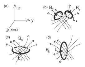
Figure 5: (a) Parameter space. (b) Illustrative effective magnetic field lines for spin up and down. The loops ${\mathbb{L}}_{\uparrow}$ and ${\mathbb{L}}_{\downarrow}$ correspond to pumping of spin up and down electrons, respectively, from left to right. (c) The field lines for charge pumping are obtained by adding the spin up and spin down field lines. The loop ${\mathbb{L}}_{c}$ corresponds to pumping of charge, i.e., unpolarized electrons. (d) The effective magnetic lines for spin. The loop ${\mathbb{L}}_{s}$ winds around the spin lines but, in total, it does not wind around the charge lines. Thus it corresponds to pure spin pumping without charge transfer.

V Application to Two Dimensional Electron Gas

In the preceding sections we have performed a general classical analysis of spin and charge pumps. We have argued that with sufficiently strong dephasing our analysis is valid. In this section we will apply the general theory [Eqs. (IV) and (32)] to a 2DEG and propose a realization of a spin battery.Cou The pumping parameters will be $x=\alpha$ determining the asymmetry between the contacts connecting the 2DEG to the left and right leads, $y=V_{g}e$ being a plunger gate and $z=h=g\mu_{B}B$ being the Zeeman energy associated with an in-plane magnetic field.

To find $\vec{B}^{\rm{eff}}_{\sigma}$ we have to calculate the dependence of the charge of the 2DEG on the pumping parameters, $\vec{\nabla}Q_{\sigma}$ [see Eq. (IV)]. The density of particles of each spin in the system, $n_{\sigma}$, is determined by the grand canonical ensemble average, and thus it is a function of the chemical potentials and of the parameters $\vec{r}=(x,y,z,...)$: $n_{\sigma}=n_{\sigma}(\mu_{\uparrow},\mu_{\downarrow},\vec{r})$ or $\mu_{\sigma}=\mu_{\sigma}(n_{\uparrow},n_{\downarrow},\vec{r})$. In the 2D case $Q_{\sigma}=n_{\sigma}eA$ where $A$ is the 2DEG area. The differentials $d\vec{r}$, $dn_{\sigma}$ for which the system remains at equilibrium satisfy $d\mu_{\sigma}=\sum_{\sigma^{\prime}}\partial\mu_{\sigma}/\partial n_{\sigma^{\prime}}|_{n_{\bar{\sigma}^{\prime}},\vec{r}}\cdot dn_{\sigma^{\prime}}+\vec{\nabla}\mu_{\sigma}|_{n_{\uparrow},n_{\downarrow}}\cdot d\vec{r}=0$. This leads to the equality

$$\vec{\nabla}Q_{\sigma}\equiv\frac{\partial Q_{\sigma}}{\partial x_{i}}=-eA\sum_{\sigma^{\prime}}D_{\sigma\sigma^{\prime}}\vec{\nabla}\mu_{\sigma^{\prime}}|_{n_{\uparrow},n_{\downarrow}},$$ (33)

where the thermodynamical density of states tensor (DOS) was introduced,

$$D_{\sigma\sigma^{\prime}}\equiv\frac{\partial n_{\sigma}}{\partial\mu_{\sigma^{\prime}}}.$$ (34)

The quantity $(\nabla\mu_{\sigma})_{i}$ is referred as the $r_{i}$ inverse compressibility of spin $\sigma$.

When the energy is given explicitly as function of $n_{\sigma}$ and $r_{i}$ we can obtain the chemical potential, the $r_{i}$ inverse compressibility of spin $\sigma$ and the DOS tensor:

$$\mu_{\sigma} = \partial_{n_{\sigma}}E(n_{\uparrow},n_{\downarrow},\vec{r}),$$

$$(\nabla\mu_{\sigma}|_{n_{\uparrow},n_{\downarrow}})_{i} = \partial^{2}_{n_{\sigma},r_{i}}E(n_{\uparrow},n_{\downarrow},\vec{r}),$$

$$F_{\sigma,\sigma^{\prime}} = \frac{\partial\mu_{\sigma}}{\partial n_{\sigma^{\prime}}};\qquad\textbf{D}=\textbf{F}^{-1}.$$ (35)

Assuming that the pumping parameters influence the energy of the system only via the terms $-e(n_{\uparrow}+n_{\downarrow})V_{g}-h(n_{\uparrow}-n_{\downarrow})$ then from Eq. (V) it follows $(\nabla\mu_{\sigma}|_{n_{\uparrow},n_{\downarrow}})_{y}=-1$ and $(\nabla\mu_{\sigma}|_{n_{\uparrow},n_{\downarrow}})_{z}=-\sigma$ with $\sigma=\pm 1$. Using $D_{\downarrow\uparrow}=D_{\uparrow\downarrow}$ and Eq. (IV) we get

$$\vec{B}^{\rm{eff}}_{\sigma} = eA\bigl{(}0,\sigma(D_{\sigma\overline{\sigma}}-D_{\sigma\sigma}),D_{\sigma\sigma}+D_{\sigma\overline{\sigma}}\bigr{)}$$

$$\vec{B}^{\rm{eff}}_{c} = eA(0,D_{\downarrow\downarrow}-D_{\uparrow\uparrow},D_{\uparrow\uparrow}+D_{\downarrow\downarrow}+2D_{\uparrow\downarrow})$$

$$\vec{B}^{\rm{eff}}_{s} = eA(0,2D_{\uparrow\downarrow}-D_{\uparrow\uparrow}-D_{\downarrow\downarrow},D_{\uparrow\uparrow}-D_{\downarrow\downarrow}),$$ (36)

with $x=\alpha$, $y=eV_{g}$, $z=h$ and $\overline{\sigma}=-\sigma$. Together with Eq. (IV) we can express the pumped current, $I_{\sigma}$, in terms of the DOS tensor.

There are some interesting relations concerning the DOS tensor: in a pumping process in which $h$ (Zeeman energy) remains constant we find that only the third component of $\vec{B}^{\rm{eff}}$ contributes. Using Eq. (V), the ratio between the spin and charge currents in this case is

$$\frac{I_{s}}{I_{c}}=\frac{B^{\rm{eff}}_{s,z}}{B^{\rm{eff}}_{c,z}}=\frac{D_{\uparrow\uparrow}-D_{\downarrow\downarrow}}{D_{\uparrow\uparrow}+D_{\downarrow\downarrow}+2D_{\uparrow\downarrow}}.$$ (37)

In equilibrium we have $\mu_{\uparrow}=\mu_{\downarrow}\equiv\mu$. MacDonald showed MacDonald (1999) that the inverse magnetic compressibility, $\frac{\partial\mu}{\partial h}|_{n_{\uparrow}+n_{\downarrow}}$, is given by minus the expression in Eq. (37).
Similarly, at constant $V_{g}$ one can verify that $\frac{I_{s}}{I_{c}}=\frac{\partial\mu}{\partial h}|_{n_{\uparrow}-n_{\downarrow}}$. Therefore measurement of charge and spin pumping currents reveals thermodynamical properties of the system.

Now we will evaluate the spin and charge pumped currents in a 2DEG relying on the Hartree-Fock approximation for its energy: Stern (1973)

$$E(n_{\uparrow},n_{\downarrow},y,z) = \frac{n^{2}_{\uparrow}+n^{2}_{\downarrow}}{2D_{0}}+\frac{e^{2}(n_{\uparrow}+n_{\downarrow})^{2}}{2\tilde{C}}-{}$$

$$-\frac{8e^{2}(n^{3/2}_{\uparrow}+n^{3/2}_{\downarrow})}{3\sqrt{\pi}} - y(n_{\uparrow}+n_{\downarrow})-z(n_{\uparrow}-n_{\downarrow}),$$ (38)

where $D_{0}^{-1}=2\pi\hbar^{2}/m^{*}$. The first term is the kinetic energy, the second and third terms are the Hartree and the exchange interactions respectively, the forth term describes interaction with an external gate potential $eV_{g}=y$ and the last term describes interaction with an external magnetic field $h=g\mu_{B}B=z$. As we will see, the negative sign of the exchange term increases the magnetic susceptibility at low densities.

V.1 Non-interacting electrons

To discuss the noninteracting case we disregard the terms $\propto e^{2}$ in Eq. (V). One finds then using Eq. (V) that $\textbf{D}=\left(\begin{array}[]{cc}D_{0}&0\\ 0&D_{0}\\ \end{array}\right)$. Equation (V) gives the effective magnetic fields, in units of $eAD_{0}$ (charge per unit energy),

$$\vec{B}^{\rm{eff}}_{\sigma}=(0,-\sigma,1)\qquad\vec{B}^{\rm{eff}}_{c}=(0,0,2)\qquad\vec{B}^{\rm{eff}}_{s}=(0,-2,0).$$ (39)

The facts that $\vec{B}^{\rm{eff}}_{c}\|z$ and $\vec{B}^{\rm{eff}}_{s}\|y$ ($y=h$, $z=V_{g}$) mean that a small loop pointing in the $z$ direction (changing $\alpha$ and $V_{g}$) produces only charge current, and a small loop pointing in the $y$ direction (changing $\alpha$ and $h$) produces a pure spin current. (The direction of a infinitesimal loop is normal to the plane of the loop.)

To estimate the pumped currents for oscillating $\alpha$ and $V_{g}$ or magnetic field $B$ we use the expression $I_{c,s}=2\tau^{-1}eAD_{0}\delta r_{c,s}\delta\alpha$ derived from Eqs. (IV) and (39). Here the energy $\delta r_{c}$ is $\delta V_{g}e$, when only charge is pumped, and $\delta r_{s}$ is $\delta h$, when only spin is pumped.

If we assume that the left-right resistors of the pump oscillate with maximal amplitude, $\delta\alpha=1$, and we consider a GaAs sample (g=-0.44) of area $A=1\mu m^{2}$, then the charge current obtained for $\delta V_{g}=3mV$ and frequency $\tau^{-1}=10GHz$ is $1.3\mu A$. At high frequencies it is difficult experimentally to produce oscillatory magnetic field with a sizable Zeeman energy. Thus, for a magnetic field of order $\delta B=1mT$ and frequency $\tau^{-1}=10KHz$ the spin pumped current is very small $\sim.5~{}10^{-15}A$.

V.2 Capacitive interaction

The simplest way to consider the Coulomb interaction is performed by adding a capacitive term to the Hamiltonian. Thus, adding the second term in Eq. (V) one has in units of $eAD_{0}$

$$\vec{B}^{\rm{eff}}_{\sigma} = (0,-\sigma,1/(1+2D_{0}e^{2}/\tilde{C}))$$

$$\vec{B}^{\rm{eff}}_{c} = (0,0,2/(1+2D_{0}e^{2}/\tilde{C}))$$

$$\vec{B}^{\rm{eff}}_{s} = (0,-2,0).$$ (40)

The observation that the magnitude of $\vec{B}^{\rm{eff}}_{c}$ has decreased reflects the fact that the energy needed to add charge to the system is now larger. On the other hand, $\vec{B}^{\rm{eff}}_{s}$ and hence the spin current are unaffected by the capacitance term.

The capacitance between the 2DEG and the gate separated one from the other by a distance $d$ is $C=\frac{\varepsilon A}{2\pi d}$. Then, the reduction factor $1+2D_{0}e^{2}/\tilde{C}$ can be written as $1+\frac{2d}{a_{0}^{\rm{eff}}}$ where $a_{0}^{\rm{eff}}$ is the effective Bohr radius $\approx 100$Å  in GaAs. For a separation of $d=1000$Å  the reduction factor is $20$. An estimate for the pumped charge in the presence of the capacitance with $\delta V_{g}=30mV$, under the conditions specified above, yields $I_{c}\simeq 0.66\mu A$.

In contrast to biased transport, where the conductivity is proportional to the aspect ratio in two dimensions, the current of the pump is proportional to the area $A$ as can be seen in the pre-factor of $\vec{B}^{\rm{eff}}$. There are two reasons to bound the area of the pump from above. One is that spin-flip events may spoil the spin polarization in too big samples. This restricts the typical lengths to $\sim\mu m$.Prinz (1998) The other restriction comes from the adiabatic condition, which for the simple circuit of Fig. (1) reads $RC\ll\tau$, where the capacitance is proportional to the area $A$. Rewriting the energy per unit area in terms of density, $n=n_{\uparrow}+n_{\downarrow}$ and magnetization, $m=n_{\uparrow}-n_{\downarrow}$, as

$$E(n,m) = \left[m-m_{0}(h)\right]^{2}\frac{1}{4D_{0}}$$ (41)

$$+ \left[n-n_{0}(V_{g})\right]^{2}\left(\frac{1}{4D_{0}}+\frac{e^{2}}{2\tilde{C}}\right),$$

where $n_{0}$ and $m_{0}$ are the average density and magnetization respectively, we can read off the effective capacitances corresponding to charge, $C_{c}=(\frac{1}{C}+\frac{1}{2AD_{0}e^{2}})^{-1}$, and to spin, $C_{s}=2AD_{0}e^{2}$, where $C=\tilde{C}A$. We see that $C_{s}>C_{c}$, thus the adiabatic condition $R\max\{C_{c},C_{s}\}\ll\tau$ becomes $A\ll\frac{\pi\tau a_{0}^{\rm{eff}}}{\varepsilon R}$. For the above mentioned conditions with $R\equiv R_{L}\parallel R_{R}=1K\Omega$, the adiabatic bound is $A\ll 400\mu m^{2}$.

V.3 Exchange interaction

The next step is to include the exchange term, the third in Eq. (V). Now the DOS tensor depends on electron density: $\textbf{F}=\textbf{D}^{-1}$ and $F_{\sigma\sigma`}=\delta_{\sigma\sigma`}D_{0}^{-1}+\frac{e^{2}}{\tilde{C}}-\delta_{\sigma\sigma`}\frac{2e^{2}n^{-1/2}_{\sigma}}{\sqrt{\pi}}$, which is different from the noninteracting 2D systems, where the DOS is constant. The dependence on density leads to a spontaneous magnetization at low densities corresponding to $r_{s}\cong 2$.MacDonald (1999) The spontaneous magnetization occurs in our model due to the following facts: (i) at constant density $n=n_{\uparrow}+n_{\downarrow}$ the exchange term is minimized for maximal $|m|$, i.e., for full polarization; (ii) in sufficiently low densities the exchange term dominates, since it behaves as $n^{3/2}$ and the others as $n^{2}$.

Before the spontaneous magnetization occurs application of magnetic field strongly polarizes the spins $(n_{\uparrow}\neq n_{\downarrow})$ and hence $D_{\uparrow\uparrow}-D_{\downarrow\downarrow}\propto n^{-1/2}_{\uparrow}-n^{-1/2}_{\downarrow}\neq 0$. This imbalance between the spin up and spin down populations at weak magnetic field becomes stronger at low densities. Using Eq. (V) we see that except for special points in parameter space it is not true that $\vec{B}^{\rm{eff}}_{c}\|z$ and $\vec{B}^{\rm{eff}}_{s}\|y$. From the last fact it follows that one can achieve spin current without varying magnetic field. This spin current is proportional to $D_{\uparrow\uparrow}-D_{\downarrow\downarrow}$ and becomes larger at low densities.

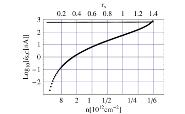
Figure 6: Spin current (big dots) ($\propto D_{\uparrow\uparrow}-D_{\downarrow\downarrow}$) and charge current (small dots) ($\propto D_{\uparrow\uparrow}+D_{\downarrow\downarrow}+2D_{\uparrow\downarrow}$) as function of density in a 2DEG according to the Hartree Fock approximation.

Following the last observation we calculated $I_{s}$ and $I_{c}$ as function of $r_{s}=\frac{1}{a_{0}^{\rm{eff}}\sqrt{\pi n}}$ at a constant magnetic field of $1T$. The conditions were similar to those specified in Sec. V.1 with $d=1000$Å, $\delta V_{g}=30mV$ and $\delta\alpha=1$. The results are plotted in Fig. 6. The charge current is almost invariant $I_{c}\simeq 0.66\mu A$. On the other hand, as explained in the previous paragraph, $I_{s}$ grows rapidly as the density is decreased until the ground state becomes ferromagnetic at $r_{s}\approx 1.4$ (the critical $r_{s}$ is now smaller due to the magnetic field).

We do not expect the Hartree-Fock approximation to be reliable for $r_{s}>1$. Monte Carlo calculations Tanatar and Ceperley (1989) show that, in reality this instability does not occur until much lower densities are reached. For $r_{s}=3/4$ we have $I_{s}=15.6nA$. It should be emphasized that the existence of $I_{s}$ is a consequence of the interactions between electrons in two dimensions. Notice that this spin current flows in the background of a large charge current of $0.64\mu A$ and may be hard to detect.

This difficulty can be resolved by a manipulation of the puming contour, using the fact that though the spin current is small, i.e., $B^{\rm{eff}}_{s}\ll B^{\rm{eff}}_{c}$, it is rapidly varying at low densities, $\frac{d}{dV_{g}}B^{\rm{eff}}_{s}\gg\frac{d}{dV_{g}}B^{\rm{eff}}_{c}$. (In Fig. 6 one can see how these quantities depend on density.) According to our topological interpretation, a small loop in parameter space probes the effective magnetic field lines passing through it. In order to probe the derivative of $B^{\rm{eff}}$, and not its magnitude, we will use a figure $8$ shaped trajectory whose equation in the $(\alpha,V_{g})$ plane is $\alpha(t)=\delta\alpha\sin(2\omega t)$, $V_{g}(t)=\delta V_{g}\sin(\omega t)$. Basically, this trajectory is composed of two adjacent loops with opposite directions. Applying such a pumping trajectory for the case of the 2DEG, means the following: in the first half of the period (one loop) we pump a charge with small polarization, as we found in our previous calculation at $r_{s}=3/4$. In the second half we pump a nearly equal amount of charge to the opposite direction, since the direction of the second loop is reversed. In the second part, however, the average density is different, thus the spin polarization is different. The excess spins may lead to a pure spin current.

The calculation for the pumped currents with the figure $8$ shaped loop, as defined above with $\delta\alpha=1/2$ and $\delta V_{g}=50mV$ yields $I_{c}=1.2nA$, $I_{s}=5.2nA$, $\frac{I_{s}}{I_{c}}=4.3$. In order to cancel the residual $1.2nA$ charge current we will consider an asymmetric figure $8$ shaped loop. This can be done using the parametrization in the $(\alpha,V_{g})$ plane given above with an additional term in $V_{g}$ equal to $\varepsilon\delta V_{g}|\sin(\omega t)|$, where the asymmetry of the trajectory is determined by the parameter $|\varepsilon|<1$. We find that $\frac{I_{s}}{I_{c}}$ diverges at $\varepsilon_{0}\cong-10^{-3}$. However, getting exactly to the point where the charge current is cancelled requires a fine tuning of $\varepsilon$. For example, to obtain $|\frac{I_{s}}{I_{c}}|>40$, the parameter $\varepsilon$ should be close to $\varepsilon_{0}$ as $|\varepsilon-\varepsilon_{0}|<2\times 10^{-4}$. This means that a resolution of about $10\mu V$ in the gates voltage is required.

V.4 Temperature effects

We would like to estimate the temperature needed for the operation of the spin pump discussed in Sec. V.3. Consider the quadratic part of Eq. (V), given in Eq. (41). The thermal smearing of the magnetization $m$ is equal to $\Delta m_{T}\simeq\sqrt{\frac{D_{0}K_{B}T}{A}}$ (The presence of the exchange term does not change $\Delta m_{T}$ significantly). In the pumping process the parameters oscillate and change the magnetization $m$ during the period with an amplitude $\Delta m_{P}$, which is related to the pumped spin current by $\Delta m_{P}\simeq\frac{I_{s}\tau}{Ae}$. We impose that the thermal smearing of $m$ is small relative to the parameters induced oscillations in $m$, i.e., $\Delta m_{T}\ll\Delta m_{P}$. This yields $T\ll(\frac{I_{s}\tau}{e})^{2}\frac{1}{K_{B}D_{0}A}\cong 10K$ where $I_{s}=5.2nA$ was used. Finally, the thermal smearing of the density $n$ is smaller than $\Delta m_{T}$ by the factor $\sqrt{\frac{C_{c}}{C_{s}}}\cong 4.4$ for the above specified conditions.

VI Summary

We analyzed classical non-coherent pumps and discussed their connection with quantum pumps using a dephasing model. Our classical method can include electron-electron interactions and allows to study the effect of exchange interaction on spin pumping. We expressed the classical pumped spin current in terms of the thermodynamic DOS tensor of the system, and gave a topological interpretation to it in terms of effective “magnetic” flux through trajectory loops in the space of the parameters that control the pump [see Eq. (II)]. We analyzed in detail the case of 2DEG GaAs and found that any combination of charge and spin currents can be obtained by choosing appropriate trajectory in parameter space. In particular one can choose a trajectory that corresponds to a pure spin current, which has magnitude of order of nano-Ampers.

VII acknowledgement

We are grateful to Alessandro Silva for many discussions at the initial stages of the research, and to Ora Entin-Wolman, Amnon Aharony, Yehoshua Levinson, Yoseph Imry, Charles Marcus, Felix von Oppen and Jens Koch for useful comments. Special thanks to David J. Thouless for the enlighten remark concerning the topological interpretation of the spin pump.

This work was supported by Minerva, by German Israeli DIP C 7.1 grant and by the Israeli Science Foundation via Grant No.160/01-1.

Appendix A Pumped currents Vs. Bias currents

According to Einstein’s relation the current of spin $\sigma=\uparrow,\downarrow$ is

$$I_{\rm{bias},\sigma}/V_{\rm bias}=e^{2}D_{\mathrm{if}}\frac{\partial n_{\sigma}}{\partial\mu}~{}\times~{}[\rm{aspect~{}ratio}],$$ (42)

where ${D_{\mathrm{if}}}$ is the diffusion constant. Using the definition of the DOS tensor, Eq. (34), we find that in equilibrium ($\mu_{\uparrow}=\mu_{\downarrow}\equiv\mu$) we have $\frac{\partial n_{\sigma}}{\partial\mu}=\sum_{\sigma^{\prime}}D_{\sigma\sigma^{\prime}}$.

Assuming that the diffusion constant is spin independent we find, [similar to Eq. (37) for the case of pumps]

$$\frac{I_{\rm bias}^{s}}{I_{\rm bias}^{c}}\equiv\frac{I_{\rm{bias},\uparrow}-I_{\rm{bias},\downarrow}}{I_{\rm{bias},\uparrow}+I_{\rm{bias},\downarrow}}=\frac{D_{\uparrow\uparrow}-D_{\downarrow\downarrow}}{D_{\uparrow\uparrow}+D_{\downarrow\downarrow}+2D_{\downarrow\uparrow}}.$$ (43)

This shows that bias currents and classical pumped currents have similar expressions in terms of the DOS tensor, cf Eq.(V). Now we will show that a pure spin current, on which we elaborated in Sec. V.3 for the case of pumping, can be obtained by an oscillatory bias together with an in-phase oscillating gate.

Consider an AC biased 2DEG in a constant magnetic field, where a gate $V_{g}$ oscillates in phase with the bias: $V_{\rm{bias}}(t)=V_{b}\sin(\omega t)$, $V_{\rm{gate}}(t)=V_{g}\sin(\omega t)$. Due to the oscillating gate a rectified DC component in the current will appear. Using Einstein’s relation, this DC current is given by

$$\langle I_{c}\rangle = e^{2}D_{\mathrm{if}}\langle(D_{\uparrow\uparrow}+D_{\downarrow\downarrow}+2D_{\downarrow\uparrow})(t)V_{\rm{bias}}(t)\rangle~{}\times~{}[\rm{a.~{}r.}]$$

$$\langle I_{s}\rangle = e^{2}D_{\mathrm{if}}\langle(D_{\uparrow\uparrow}-D_{\downarrow\downarrow})(t)V_{\rm{bias}}(t)\rangle~{}\times~{}[\rm{a.~{}r.}]$$ (44)

where $\langle\rangle$ denotes time average over a period and we assumed that the diffusion constant does not depend on $V_{\rm bias}$ or $V_{\rm gate}$.

Near the magnetic instability the spin current $\propto D_{\uparrow\uparrow}-D_{\downarrow\downarrow}$ is very susceptible to changes in $V_{g}$ while the charge current $\propto D_{\uparrow\uparrow}+D_{\downarrow\downarrow}+2D_{\downarrow\uparrow}$ is nearly constant (see Fig. 6). As a result, the charge flowing in one half of the period cancels the charge flowing in the second half, while a finite amount of spins is transferred from left to tight.

This rectification Rec effect is based on the same mechanism as the adiabatic pumping effect considered in Sec. V.3. Both effects are proportional to the interaction strength.

We will show now that the two effects of pumping and rectification (bias) produce currents of the same order, provided that (i) the pumping frequency saturates the adiabatic condition, $\tau=RC$ and (ii) the pumping gate, the rectification gate and the bias oscillate with similar amplitudes.

First consider a simple pumping loop in which the asymmetry parameter $\alpha$ and the pumping gate oscillate out of phase with $\delta\alpha=1$, $\delta V_{g}=V$. When the adiabatic condition is saturated, $\tau=RC$, the pumped current in the circuit of Fig. 1, given in Eq. (12), is $I_{\rm{pump}}=\tau^{-1}CV\delta\alpha=V/R$. Using Ohm‘s law we see that the DC current flowing due to a DC bias $V$ in the same circuit is of the same order, i.e., $I_{\rm{bias}}=V/2R$, where we assumed $R\equiv R_{L}\parallel R_{R}\simeq R_{L}/2\simeq R_{R}/2$ for simplicity.

Second, let us compare the spin currents for pumping with a figure 8 shaped loop and for rectification (i.e., bias voltage) with an oscillating gate. We can apply the above argument for each half period of either pumping or rectification processes: for pumping, each half period consists of one of the two loops of the figure 8. In each such loop the amplitude of the gate oscillation is half of the oscillation in the entire period. For the case of rectification, in each half period the averaged bias is of the order of the maximal AC amplitude. In both cases, the density varies between the two halves of the periods: the voltage providing different densities corresponds to (i) the distance between the centers of the two loops in figure 8 for the case of pumping; (ii) the oscillations of the gate in the case of rectification. Thus when the pumping gate, the rectification gate and the bias oscillate with similar amplitudes similar spin currents will be created in the pumping and in the rectification processes.

To conclude, unless biasing of the system is unwanted, one can obtain spin current either by the pumping effect discussed in Sec. V.3 or by the rectification effect combined with an oscillating gate described here.

On the other hand, as is seen in Appendix B, for long systems adiabatic pumping is more feasible than application of bias, since it requires only small voltages.

Appendix B Connection with non-linear response theory

In this section we compare our results to other theories Kamenev and Oreg (1995); von Oppen et al. (2001) that evaluate non linear response to an external potential at wave number $k$ and frequency $\omega$.

We start by analyzing the circuit of Fig. 3 in the continuous limit, with the assumptions (i) $R_{m}=R(V_{g~{}m})$ and $C_{m}=C(V_{g~{}m})$ so that the varying parameters are $\{V_{g~{}m}\}$; (ii) periodic boundary conditions: $R_{1}$ is connected to $R_{N}$.

The continuous version of the current conservation in the junctions of Fig. 3 is, in the adiabatic limit,

$$\frac{dI(r,t)}{dr}=-\tilde{C}\bigl{(}V_{g}(r,t)\bigr{)}\dot{V}_{g}(r,t),\quad\omega\tilde{R}\tilde{C}k^{-2}\ll 1,$$ (45)

where $I(r)$ is the current along the circuit and $\tilde{C},\tilde{R}$ are the capacitance and resistance per unit length respectively. To estimate the adiabatic condition we use the characteristic length scale $k^{-1}$. The periodic boundary conditions imply

$$\int_{0}^{l}drI(r,t)\tilde{R}\bigl{(}V_{g}(r,t)\bigr{)}=0,$$ (46)

where $l$ is the length of the system. Integrating Eq. (45) and substituting into Eq. (46) we have:

$$I(0,t)l\tilde{R}(\bar{V}_{g}(t)) = \int_{0}^{l}dr\tilde{R}\bigl{(}V_{g}(r,t)\bigr{)}$$ (47)

$$\times \int_{0}^{r}dr^{\prime}\tilde{C}\bigl{(}V_{g}(r^{\prime},t)\bigr{)}\dot{V_{g}}(r^{\prime},t),$$

where $\bar{V_{g}}(t)=l^{-1}\int_{0}^{l}drV_{g}(r,t)$.

We proceed by assuming that the potential $V_{g}(r,t)$ depends on two parameters $x,y$ as

$$V_{g}(r,t)=x(t)\sin(kr)+y(t)\cos(kr),$$ (48)

and take $\tilde{C}\bigl{(}V_{g}(r,t)\bigr{)}=\tilde{C}$ to be a constant. The integral over $r^{\prime}$ in Eq. (47) yields

$$\frac{\tilde{C}}{k}\left[\dot{x}(t)\bigl{(}1-\cos(kr)\bigr{)}+\dot{y}(t)\sin(kr)\right],$$ (49)

and the integral over $r$ yields

$$I(0,t)=\frac{\tilde{C}\tilde{R}^{\prime}}{2k\tilde{R}}\bigl{(}x(t)\dot{y}(t)-y(t)\dot{x}(t)\bigr{)}+\frac{\tilde{C}}{k}\dot{x},$$ (50)

where we expanded $\tilde{R}$ around $\bar{V}_{g}=0$ as $\tilde{R}(V_{g})=\tilde{R}+\tilde{R}^{\prime}V_{g}$. Integrating Eq.(50) over one period as done in Eq. (II), we get the charge per period for small area $\mathbb{S}$:

$$Q_{p}=\frac{\tilde{C}\tilde{R}^{\prime}}{k\tilde{R}}\int_{\mathbb{S}}dxdy\Rightarrow$$

$$j_{\rm DC}=\frac{\tilde{R}^{\prime}\tilde{C}}{\tilde{R}}\frac{\omega}{k}V^{2}.$$ (51)

in the last equality we have assumed that $x(t)=\sqrt{2}V\cos(\omega t)$, $y(t)=\sqrt{2}V\sin(\omega t)$.

We can compare our results to the non liner response theory. Ignoring coherent effects,Kamenev and Oreg (1995) the current response to a time and space dependent potential $V(r,t)$ is $j(r,t)=-\sigma[n(r,t)]\nabla V(r,t)$. If $V(r,t)$ induces a density polarization given by $\delta n(k,\omega)=-\Pi(k,\omega)eV(k,\omega)$, the DC response current is given by Kamenev and Oreg (1995); von Oppen et al. (2001)

$$j_{\rm{DC}}=\sum_{k,\omega}\frac{d\sigma}{den}k\Im\Pi(k,\omega)|eV(k,\omega)|^{2}.$$ (52)

We take now the diffusive polarization operatorKamenev and Oreg (1995) in the limit $D_{\rm if}k^{2}\gg\omega$, this gives $\Im\Pi(k,\omega)\rightarrow-\frac{\omega}{D_{\rm if}k^{2}}\frac{dn}{d\mu}$. Thus,

$$\begin{array}[]{ccccc}j_{\rm{DC}}&=&-\frac{d\sigma}{d\mu}\frac{d\mu}{den}\frac{1}{D_{\rm if}}&e^{2}\frac{dn}{d\mu}&\frac{\omega}{k}V^{2}\\ &=&\frac{\tilde{R}^{\prime}}{\tilde{R}}&\tilde{C}&\frac{\omega}{k}V^{2},\end{array}$$ (53)

which is identical to Eq. (B). Since $D_{\rm if}=\frac{\sigma}{e^{2}dn/\mu}=1/(\tilde{R}\tilde{C})$ the limit $D_{\rm if}k^{2}\gg\omega$ is identical to the adiabatic limit, Eq. (45).

References

- Rorres (2000) C. Rorres, ASCE Journal of Hydraulic Engineering 126, 72 (2000).
- Thouless (1983) D. J. Thouless, Phys. Rev. B 27, 6083 (1983).
- (3) B. Spivak, F. Zhou, and M. T. B. Monod, Phys. Rev. B 51, 13226 (1995).
- (4) P. W. Brouwer, Phys. Rev. B 58, R10135 (1998).
- (5) J. E. Avron, A. Elgart, G. M. Graf, and L. Sadum, Phys. Rev. B 62, 10618 (2000).
- (6) O. Entin-Wohlman, A. Aharony, and Y. Levinson, Phys. Rev. B 65, 195411 (2002).
- Moskalets and Buttiker (2001) M. Moskalets and M. Buttiker, Phys. Rev. B 64, 201305 (2001).
- Cremers and Brouwer (2001) J. N. H. J. Cremers and P. W. Brouwer, Phys. Rev. B 65, 115333 (2001).
- Brouwer et al. (2002) P. W. Brouwer, J. N. H. J. Cremers, and B. I. Halperin, Phys. Rev. B 65, 081302 (2002).
- Jauho et al. (1994) A.-P. Jauho, N. S. Wingreen, and I. Meir, Phys. Rev. B 50, 5528 (1994).
- Aleiner and Andreev (1998) I. L. Aleiner and A. V. Andreev, Phys. Rev. Lett. 81, 1286 (1998).
- Sharma and Chamon (2001) P. Sharma and C. Chamon, Phys. Rev. Lett. 87, 096401 (2001).
- Kouwenhoven et al. (1991) L. P. Kouwenhoven, A. T. Johnson, N. C. van der Vaart, C. J. P. M. Harmans, and C. T. Foxon, Phys. Rev. Lett. 67, 1626 (1991).
- Pothier et al. (1991) H. Pothier, P. Lafarage, P. F. Orfila, C. Urbina, D. Estive, and M. H. Devoret, Physica B 169, 573 (1991).
- Switkes et al. (1999) M. Switkes, C. M. Marcus, K. Campman, and A. C. Gossard, Science 283, 1905 (1999).
- Brouwer (2001) P. W. Brouwer, Phys. Rev. B 63, 121303 (2001).
- (17) We would like to emphasize the difference between pumping and rectification. By definition a pump converts AC variations of the parameters of an unbiased system into a net DC current. On the other hand rectification converts an AC bias into a DC current. The pumping electrical circuit that we discuss works in the absence of an AC bias, so our effect is that of pumping. A qualitative difference between pumping and rectification currents is that the average pumping current is proportional to the frequency, , while the DC current in an AC-biased-diode does not depend on the frequency.
- Sharma and Brouwer (2003) P. Sharma and P. W. Brouwer, Phys. Rev. Lett. 91, 166801 (2003).
- (19) E. Sela and Y. Oreg, in preparation.
- Buttiker (1986) M. Buttiker, Phys. Rev. B 33, 3020 (1986).
- (21) We use the 4 leg version for controlled dephasing instead of the 3 leg model since this enables us to obtain perfect dephasing. (see remark in Buttiker (1986)).
- Das et al. (2003) S. Das, S. Rao, and D. Sen (2003), cond-mat/0311563.
- Landauer (1957) R. Landauer, IBM J. Res. Dev. 1, 223 (1957).
- (24) Consider for example the case . In that case since and no pumping current flows through reservoirs we have and have to solve two simple linear equations for and , that together with Eq. (21) give Eq. (III).
- (25) Treatment of Coulomb-blockade situatiuons will take place in a future work Sela and Oreg .
- MacDonald (1999) A. H. MacDonald, condmat p. 9912391 (1999).
- Stern (1973) F. Stern, Phys. Rev. Lett. 30, 278 (1973).
- Prinz (1998) G. A. Prinz, Science 282, 1660 (1998).
- Tanatar and Ceperley (1989) B. Tanatar and D. M. Ceperley, Phys. Rev. B 39, 5005 (1989).
- Kamenev and Oreg (1995) A. Kamenev and Y. Oreg, Phys. Rev. B 52, 7516 (1995).
- von Oppen et al. (2001) F. von Oppen, S. H. Simon, and A. Stern, Phys. Rev. Lett. 87, 106803 (2001).