Rabi Oscillations in Systems with Small Anharmonicity

Abstract

When a two-level quantum system is irradiated with a microwave signal, in resonance with the energy difference between the levels, it starts Rabi oscillation between those states. If there are other states close, in energy, to the first two, the Rabi signal will also induce transition to those. Here, we study the probability of transition to the third state, in a three-level system, while a Rabi oscillation between the first two states is performed. We investigate the effect of pulse shaping on the probability and suggest methods for optimizing pulse shapes to reduce transition probability.

I Introduction

Most qubits (i.e. basic elements in a quantum computer) are not true two-level systems. Yet, only the first two energy states are commonly considered relevant for quantum computation. As a result, any transition to the upper levels during the gate operations is a leakage of information outside the computational space, and therefore a source of error.

One of the common methods to perform gate operations in a qubit is via Rabi oscillations Rabi . The speed of operation is determined by the Rabi frequency $\Omega_{R}$, which is proportional to the amplitude of the applied microwave signal. Rabi oscillations have been observed in many quantum systems, including superconducting qubits NECRabi ; vion ; martinis ; chiorescu ; ilichev , excitons in single quantum dots QD1 ; QD2 , and very recently single electron spins in nitrogen-vacancy defect centers in diamond jelezko .

In a multi-level quantum system, Rabi oscillations may not be limited to only the first two states. For example, in a harmonic oscillator, with equally spaced energy eigenvalues, applying a Rabi signal in resonance with the level spacings will occupy many states. When the system is strongly anharmonic, on the other hand, i.e. when the third state is far above the first two, the probability of transition will be vanishingly small.

To have a quantitative measure of anharmonicity, we define an anharmonicity coefficient by

$$\delta={(E_{21}-E_{10})/E_{10}},$$ (1)

where, $E_{ij}=E_{i}-E_{j}$, with $E_{0}$ being the ground state and $E_{i>0}$, the $i$-th excited state energy. $\delta$ is zero for a harmonic oscillator and ${\to}+\infty$ for an ideal two level system.

Not every qubit realization has large $\delta$. For example, in a current biased Josephson junction qubit martinis , $E_{21}$ is always smaller than $E_{10}$ leading to a negative $\delta$ close to zero. Charge-phase qubits also suffer from small anharmonicity, merely because of operating in the charge-phase regime; for the “quantronium” qubit of Vion et al. vion , $\delta\approx 0.2$, and for the flux based charge-phase qubit of Ref. amin , a $\delta=O(1)$ was suggested.

The purpose of this paper is to study how much smallness of $\delta$ can affect transition to the upper state, and how it can be prevented. We study the problem in a three-state quantum system with small anharmonicity. In Sec. II, we perform analytical calculations using Rotating Wave Approximation (RWA). Section III, goes beyond RWA using numerical methods. The effect of pulse shaping on the transition probabilities is addressed in Sec. IV. Section V, discusses practical examples within superconducting qubit implementations. A brief summary together with some concluding remarks are provided in Sec. VI.

II Analytical calculation

Let us consider a quantum system with three states $|i\rangle$, $i=a,b,c$, irradiated with a microwave signal in resonance with the energy difference between the first two levels. The Hamiltonian of the system is written as ($E_{c}>E_{b}>E_{a}=0$)

$$H=E_{b}|b\rangle\langle b|+E_{c}|c\rangle\langle c|+V(t)$$ (2)

where $V(t)=V_{0}e^{-i\omega_{0}t}+$ c.c. is the microwave signal ($\hbar=1$). Writing the wave function as $\psi(t)=c_{a}(t)|a\rangle+c_{b}(t)|b\rangle+c_{c}(t)|c\rangle$, the equations of motion for $c_{i}$ are

$$i\dot{c}_{a} = V_{ab}c_{b},$$

$$i\dot{c}_{b} = V_{ab}^{*}c_{a}+E_{b}c_{b}+V_{bc}c_{c},$$

$$i\dot{c}_{c} = V_{bc}^{*}c_{b}+E_{c}c_{c},$$ (3)

where $V_{ij}(t)=\langle i|V(t)|j\rangle$. We have taken $V_{ac}=0$; the transition probability will be small anyway because of large frequency difference. For simplicity, we write $E_{b}=\omega_{0}$ and $E_{c}=(2+\delta)\omega_{0}$. In this section, we assume $\delta\ll 1$ to ensure small anharmonicity.

Let us define $\tilde{c}_{b}=c_{b}e^{i\omega_{0}t}$, $\tilde{c}_{c}=c_{c}e^{i2\omega_{0}t}$, and write $V_{ab}/\omega_{0}=ue^{-i\omega_{0}t}+$ c.c. and $V_{bc}/\omega_{0}=ve^{-i\omega_{0}t}+$ c.c. Using RWA, i.e. ignoring the fast oscillating terms, we find

$$\partial_{\tau}{\tilde{c}}_{a} = -iu\tilde{c}_{b},$$

$$\partial_{\tau}{\tilde{c}}_{b} = -iu^{*}\tilde{c}_{a}-iv\tilde{c}_{c},$$

$$\partial_{\tau}{\tilde{c}}_{c} = -iv^{*}\tilde{c}_{b}-i\delta\tilde{c}_{c},$$ (4)

where $\tau=\omega_{0}t$. The equation of motion for $\tilde{c}_{b}$ can be extracted from (4):

$$\left[\partial_{\tau}^{3}+i\delta\partial_{\tau}^{2}+(|u|^{2}+|v|^{2})\partial_{\tau}+i\delta|u|^{2}\right]\tilde{c}_{b}=0.$$ (5)

Writing $\tilde{c}_{b}=ke^{-ix\tau}$, $x$ needs to satisfy

$$x^{3}-\delta x^{2}-(|u|^{2}+|v|^{2})x+\delta|u|^{2}=0.$$ (6)

General solutions are

$$x_{n}={1\over 3}\left\{\delta+2z\cos\left[\theta+(2n-1){\pi\over 3}\right]\right\},\quad n=1,2,3$$ (7)

where

$$z = \sqrt{3(|u|^{2}+|v|^{2})+\delta^{2}},$$ (8)

$$\theta = {1\over 3}\arccos\left({9\delta\left(|u|^{2}-|v|^{2}/2\right)-\delta^{3}\over z^{3}}\right).$$ (9)

To find the coefficients, let us write

$$\tilde{c}_{a} = \sum_{n=1}^{3}k_{n}e^{-ix_{n}\tau},$$

$$\tilde{c}_{b} = {1\over u}\sum_{n=1}^{3}x_{n}k_{n}e^{-ix_{n}\tau},$$

$$\tilde{c}_{c} = {1\over uv}\sum_{n=1}^{3}(x_{n}^{2}-|u|^{2})k_{n}e^{-ix_{n}\tau},$$ (10)

which satisfy (4). Assuming that the system starts from the ground state, we impose the initial conditions: $\tilde{c}_{a}=1$ and $\tilde{c}_{b}=\tilde{c}_{c}=0$, which yield

$$\sum_{n=1}^{3}k_{n}=0,\quad\sum_{n=1}^{3}x_{n}k_{n}=0,\quad\sum_{n=1}^{3}x_{n}^{2}k_{n}=|u|^{2}$$ (11)

Solving these equations for $k_{n}$, we find

$$k_{1}={|u|^{2}+x_{2}x_{3}\over(x_{1}-x_{2})(x_{1}-x_{3})}.$$ (12)

$k_{2}$ and $k_{3}$ can be obtained using the permutation $1{\to}2{\to}3{\to}1$.

Let us write $\tilde{c}_{c}=\sum\alpha_{n}e^{-ix_{n}\tau}$, where $\alpha_{n}=(x_{n}^{2}-|u|^{2})k_{n}/uv$. The probability of finding the system in the upper state is

$$P_{c}(\tau)=|\tilde{c}_{c}|^{2}=\left|\sum_{n=1}^{3}\alpha_{n}e^{-ix_{n}\tau}\right|^{2}\leq P_{\rm max}$$ (13)

where

$$P_{\rm max}=\left(\sum_{n=1}^{3}|\alpha_{n}|\right)^{2}$$ (14)

determines an upper bound for $P_{c}(\tau)$. We first study the solution is some special cases.

II.1 Case I, $\delta=0$

This is the simplest case that the problem can be solved. From (7)–(9), we find

$$x_{1}=0,\qquad x_{2,3}=\mp\Omega_{R},$$ (15)

where $\Omega_{R}=\sqrt{|u|^{2}+|v|^{2}}$. These can also be found easily from (6) directly. Using (12), we find $k_{1}=|v/\Omega_{R}|^{2}$ and $k_{2}=k_{3}=(1/2)|u/\Omega_{R}|^{2}$. As a result

$$\tilde{c}_{a} = {1\over\Omega_{R}^{2}}(|v|^{2}+|u|^{2}\cos\Omega_{R}\tau),$$

$$\tilde{c}_{b} = -i{u^{*}\over\Omega_{R}}\sin\Omega_{R}\tau,$$

$$\tilde{c}_{c} = -{u^{*}v^{*}\over\Omega_{R}^{2}}(1-\cos\Omega_{R}\tau).$$ (16)

The system oscillates with only one frequency $\Omega_{R}$. The probability of finding the system in the upper state $|\tilde{c}_{c}|^{2}$ can become large: $P_{\rm max}=4|uv|^{2}/\Omega_{R}^{4}$. This is expected in a system with zero anharmonicity.

II.2 Case II, $v=0$

Using (8)–(9), together with

$$\cos 3\theta=4\cos^{3}\theta-3\cos\theta,$$ (17)

we find $\cos\theta=-\delta/z$, which immediately gives

$$x_{1}=-|u|,\qquad x_{2}=\delta,\qquad x_{3}=|u|.$$ (18)

These could also be found directly from (6). For $k$’s, we get: $k_{1}=k_{3}=1/2$ and $k_{2}=0$, leading to

$$\tilde{c}_{a} = \cos\Omega_{R}\tau,$$

$$\tilde{c}_{b} = -i{\Omega_{R}\over u}\sin\Omega_{R}\tau,$$

$$\tilde{c}_{c} = 0.$$ (19)

The results show usual Rabi oscillation between the first two states with frequency $\Omega_{R}=|u|$. The probability of finding the system in the upper state is always zero ($P_{c}=0$), as expected because $v=0$.

II.3 Case III, $\delta\gg u,v$

In the regime $u,v\ll\delta\ll 1$, one can find asymptotic solutions. A systematic expansion in $u/\delta$ and $v/\delta$ gives

$$x_{1} = |u|\left(1-{|v|^{2}\over 2\delta^{2}}\right)-{|v|^{2}\over 2\delta}$$

$$x_{2} = -|u|\left(1-{|v|^{2}\over 2\delta^{2}}\right)-{|v|^{2}\over 2\delta}$$

$$x_{3} = \delta\left(1+{|v|^{2}\over\delta^{2}}\right)$$ (20)

Leading to the Rabi frequency

$$\Omega_{R}=|u|\left(1-{|v|^{2}\over 2\delta^{2}}\right)$$ (21)

The dependence of the Rabi frequency on the amplitude of the microwave signal now has the form

$$\Omega_{R}\propto V_{0}\left(1-\beta V_{0}^{2}\right),$$ (22)

where the coefficient $\beta$ depends on the details of the system. The deviation from the proportionality relation is a signature of transition to the upper states. Such a deviation has been experimentally observed recently in a current biased dc-SQUID structure claudon .

The probability of finding the system in the upper state is given by

$$P_{c}\approx{|v|^{2}\over\delta^{2}}\sin^{2}\Omega_{R}\tau.$$ (23)

It oscillates with the Rabi frequency $\Omega_{R}$. The maximum probability

$$P_{\rm max}\approx{|v|^{2}\over\delta^{2}}\approx\gamma\left({\Omega_{R}\over\delta}\right)^{2}$$ (24)

occurs at half a Rabi period $\tau=\pi/\Omega_{R}$, where $P_{b}$ is the largest. This is not the case for small $\delta$ (see e.g. case I). Here, $\gamma=|v/u|^{2}$ is a constant depending on the details of the Hamiltonian. In most physical systems $|v|\sim|u|$ and therefore $\gamma=O(1)$.

II.4 General case

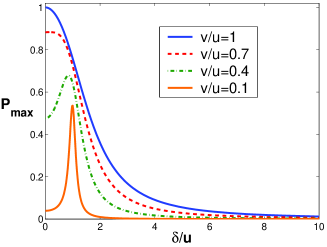
Figure 1: $P_{\rm max}$ vs $\delta/u$ for different values of $v/u$. The curves are symmetric with respect to $\delta\to-\delta$.

It is not straightforward to find a closed analytical solution for the general case. Instead we plot the results for $P_{\rm max}$, calculated using (7)–(9) together with (12) and (14). Figure 1 shows $P_{\rm max}$ as a function of $\delta/u$ with different values of $v/u$. At small $v/u$, the curves are peaked near $\delta=u$, while for larger $v/u$ the peak appears near $\delta=0$. In all cases $P_{\rm max}$ becomes very small at large $\delta/u$, as expected.

III Numerical calculation

In this section we calculate the quantum evolution of the system numerically using density matrix approach. This allows us to study the system beyond RWA and/or at large $\delta$. The dynamics of the $3\times 3$ density matrix $\rho$ is described by

$$i{d\rho\over dt}=[H,\rho].$$ (25)

We integrate this equation starting from

$$\rho_{0}=\left(\begin{array}[]{ccc}1&0&0\\ 0&0&0\\ 0&0&0\end{array}\right),$$ (26)

which describes the system at the lowest energy state. Probabilities of finding the system in different states are given by: $P_{a}=\rho_{11}$, $P_{b}=\rho_{22}$, and $P_{c}=\rho_{33}$. Figure 2 displays the time evolution of these probabilities. The fast oscillations are the effect of high frequency terms, which were ignored in the previous section due to RWA. Figure 2a shows the Rabi oscillation when $\delta=0.1$. After (almost) half a Rabi period, significant amount of the probability goes to the third state. By increasing $\delta$ to 0.5, the probability of finding the system in the upper state is significantly reduced (Fig. 2b; the curve in the figure is magnified for clarity).

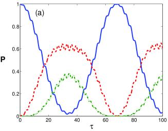
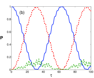
Figure 2: Probability $P_{a}$ (solid), $P_{b}=\rho_{22}$ (dashed), and $P_{c}=\rho_{33}$ (dot-dashed), as a function of time. The parameters are $u=v=0.1$, $\delta=0.1$ (a) and $\delta=0.5$ (b). For clarity, $P_{c}$ in (b) is magnified by a factor of 10.

The maximum probability of the system in the upper state is given by $P_{\rm max}={\rm Max}_{\tau}[P_{c}]$. Figure 3 shows the dependence of $P_{\rm max}$ on $\delta$. The solid lines are analytical curves using (14), and the dashed ones represent the results of numerical calculations. While the two curves coincide at small $\delta$, they soon deviate from each other as $\delta$ increases. However, the overall behavior of the curves, especially the asymptotic $P_{\rm max}\sim|v|^{2}/\delta^{2}$ dependence remains unchanged even at large $\delta$. To emphasize on this aspect, we have plotted $P_{\rm max}\delta^{2}/|v|^{2}$ vs $\delta$ in Fig. 4, for different values of parameters. All the curves overlap at large $\delta$ suggesting $P_{\rm max}\sim|v|^{2}/\delta^{2}\sim(\Omega_{R}/\delta)^{2}$, in agreement with (24); the coefficient $\gamma$, however, is now a slow function of the parameters, but still $O(1)$.

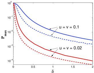
Figure 3: $P_{\rm max}$ vs $\delta$ for different values of $u$ and $v$. Solid (dashed) curves are analytical (numerical) results.

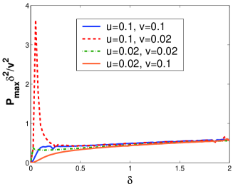
Figure 4: $P_{\rm max}\delta^{2}/|v|^{2}$ vs $\delta$ for different values of $u$ and $v$.

IV Effect of pulse shape

So far we have assumed that the microwave signal starts at $\tau=0$, and continues forever. To perform a gate operation, however, one needs to apply the Rabi signal for only a short duration of time. In that respect, our calculation can only describe hard pulses, in which the microwave switches on and off abruptly. The probability $P_{c}$ then oscillates with the pulse duration at the Rabi frequency. The maximum probability usually happens in the case of a $\pi$-rotation, i.e when the probability is maximally transferred to $|b\rangle$. A hard pulse, however, is neither practical, nor the best pulse shape, as was indicated in Ref. steffen, . Indeed, by using other types of pulses, the probability of transition to the upper level, at the end of the process, can be significantly reduced. Among a few pulse shapes examined in steffen , Gaussian pulses demonstrated the most promise. To understand the role of pulse shaping, let us compare the effect of a Gaussian pulse on the probability $P_{c}$, with that of a hard pulse, for the case of a $\pi$-rotation.

To enforce a Gaussian envelope for the microwave signal V(t), we write

$$u(\tau)=\left\{\begin{array}[]{cc}({a\Gamma/\tau_{w}})e^{-(\tau-\tau_{p}/2)^{2}/2\tau_{w}^{2}}&\ \ {\rm for}\ 0<\tau<\tau_{p}\\ 0&{\rm otherwise}\end{array}\right.,$$ (29)

where $\tau_{p}$ and $\tau_{w}$ are the duration and width of the pulse respectively, $\Gamma$ is the total angle of rotation in the Bloch sphere (e.g. $\Gamma=\pi$ for a $\pi$-rotation), and $a$ is a normalization constant.

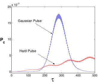
Figure 5: Probability of the third level as a function of time for a hard and a Gaussian $\pi$-pulse.

Figure 5 shows the probability $P_{c}$ as a function of time for a Gaussian and a hard pulse, both of which having the same duration and resulting in a $\pi$-rotation ($\Gamma=\pi$) at the end of the pulse. In our numerical calculation we take $v=u$, $\delta=0.05$, $\tau_{p}=500$, $\tau_{w}=\tau_{p}/6$, and $a=0.398$. These numbers correspond to the optimal pulse shape suggested in steffen . The maximum of $P_{c}$ for the Gaussian pulse, happens slightly after the center of the pulse, while in the case of the hard pulse, it occurs near the end. Although the maximum is larger for the Gaussian pulse, the probability $P_{cf}$ at the end of the process is much smaller. Orders of magnitude reduction of the final probability can be achieved using such a technique.

In Ref. steffen, , $\tau_{w}$ was fixed (to $\tau_{p}/6$ or $\tau_{p}/4$) and $\tau_{p}$ was varied to minimize $P_{cf}$. A $\tau_{p}\approx 8\pi/|\delta|$ was shown to provide the first minimum with shortest duration. Alternatively, one can fix $\tau_{p}$ and find a $\tau_{w}$ which gives minimum $P_{cf}$. This may work better for shorter pulses. For example, for $\tau_{p}=100$, $\delta=0.1$, and $v=u$, a Gaussian pulse with $\tau_{w}=\tau_{p}/6$ gives $P_{cf}=0.093$, while the minimum probability $P_{cf}=0.0026$ is achieved at $\tau_{w}=0.31\tau_{p}$ and $a=0.467$. Such a pulse shape starts and ends with jumps (see Fig. 6), but still gives smaller $P_{c}$ at the end of the process.

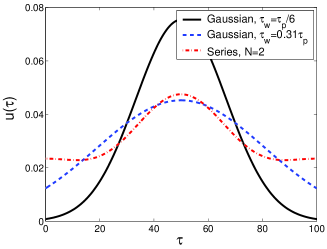
Figure 6: Pulse shapes optimized for a $\pi$-rotation with $\delta=0.1,\ \tau_{p}=100$.

A Gaussian pulse shape is not the optimal pulse shape for minimizing $P_{cf}$. One can design other pulses with more free parameters to achieve a smaller probability. To have some idea about how small can $P_{cf}$ be made by appropriately shaping the pulse, we defined an arbitrary pulse by the series

$$u(\tau)=(\Gamma/\tau_{p})\left[1+\sum_{n=1}^{N}\lambda_{n}\cos(2\pi n\tau/\tau_{p})\right].$$ (30)

Keeping only the first two terms in the series, (using the same conditions as above: $\tau_{p}=100$, $\delta=0.1$, and $v=u$) one can already reach a probability as small as $P_{cf}=1.2\times 10^{-5}$ with $\lambda_{1}=-0.3833$ and $\lambda_{2}=0.1293$ (see Fig. 6). With $N=33$ terms in the series, the probability was reduced to $2.4\times 10^{-6}$. The resulting pulse shape, shown in Fig. 7, is complicated and may not be useful experimentally. It should also be emphasized that with the pulse shape of (30), there is not a unique minimum for $P_{cf}$. Depending on the starting point and the method of minimization, one may fall into a local minimum with complicated pulse shape.

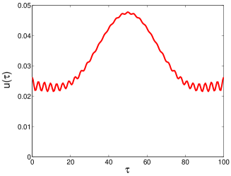
Figure 7: Pulse shape of Eq. (30), optimized with $N=33$.

Here, we only considered the case of $\Gamma=\pi$. For quantum operations, other pulses may also be required. It is not just enough to change the amplitude of the pulse, keeping its shape and duration, to obtain optimized pulses with other $\Gamma$’s. Indeed, for each type of operation, one needs to design a specific pulse shape that provides minimum $P_{cf}$.

V Discussion

In a practical quantum computer, the maximum number of operations is limited by the decoherence time of the qubits as well as the speed of operations. It is generally believed that if $\sim 10^{4}$ operations can be performed within the decoherence time, quantum computation can continue indefinitely with the help of quantum error correction algorithms. A parameter that is commonly quoted as a measure for the maximum number of operations is the quality factor of the qubits, usually defined as

$$Q_{\varphi}={1\over 2}\tau_{\varphi},$$ (31)

where $\tau_{\varphi}$ is the dephasing time of the qubit (in units of $1/\omega_{0}$). $Q_{\varphi}$, however, is related to only one type of single qubit operations, namely phase rotation. Other necessary operations such as single qubit state flip or multi-qubit gate operations are usually much slower. Even for the phase rotation, the extent to which one can control the rotation, i.e. change $E_{10}$, may be much smaller than the rotation frequency itself.

The single qubit state flip can be performed using Rabi oscillations martinis ; vion ; chiorescu or non-adiabatic evolution nakamura . The latter is fast ($\approx\omega_{0}$), but requires large anharmonicity to avoid unwanted Landau-Zener transition to the upper states. Rabi oscillations, on the other hand, are much slower, but can be used in small anharmonicity systems. It is possible to define a quality factor for the Rabi oscillations the same way as $Q_{\varphi}$ was defined in (31)

$$Q_{R}\equiv{1\over 2}\Omega_{R}\tau_{R}\approx\Omega_{R}Q_{\varphi},$$ (32)

where $\tau_{R}$ is the Rabi decay time which is typically the same order as $\tau_{\varphi}$.

In an ideal two level system, $\Omega_{R}$ is limited by the maximum allowed amplitude of the microwave signal (restricted by RWA and/or experimental limitations). Usually an $\Omega_{R}$ as large as $0.1$ or even larger is conceivable. In practical systems, especially those with small anharmonicity, however, increasing the microwave power will cause transition to the upper states as we discussed. Therefore $\Omega_{R}$ is limited by how much probability of the upper levels can be tolerated. If we restrict $P_{\rm max}$ to $\sim 10^{-4}$, then (24) gives $\Omega_{R}\sim 10^{-2}\delta$. Therefore to achieve $\Omega_{R}\sim 0.1$ ($Q_{R}\sim 0.1Q_{\varphi}$), we need a $\delta>10$. Such a large anharmonicity cannot be supported by many qubit implementations (see below for a few examples).

Using a shaped (instead of hard) pulse can significantly reduce the final $P_{c}$. To define a quality factor similar to (32), we use the fact that in the case of a hard pulse, a $\pi$-rotation is implemented when $\Omega_{R}=\pi/\tau_{p}$. We therefore define

$$Q_{\rm shaped}\equiv{1\over 2}\left({\pi\over\tau_{p}}\right)\tau_{\varphi}=\left({\pi\over\tau_{p}}\right)Q_{\varphi}.$$ (33)

Therefore a $Q_{\rm shaped}=0.1Q_{\varphi}$ requires a pulse with duration $\tau_{p}=10\pi\approx 30$ for a $\pi$-rotation. It was shown in steffen , that a Gaussian pulse with $\tau_{w}=\tau_{p}/6$ provides minimum $P_{c}$ with shortest time if $\tau_{p}\approx 8\pi/|\delta|$. A quality factor of $0.1Q_{\varphi}$ is therefore achievable in a system with $\delta\approx 0.8$. Other pulse shapes may provide better performance at smaller $\delta$, as was discussed before. Below, we provide a few examples among superconducting qubits.

In the current biased Josephson junction qubit of Ref. martinis, , the energy differences are $\omega_{10}\approx 6.9$ GHz and $\omega_{21}\approx 6.28$ GHz, leading to $\delta\approx-0.09$. Also, one can easily justify steffen that $|v|=\sqrt{2}|u|\sim|u|$, as expected. For a hard pulse, requiring $P_{\rm max}\sim 10^{-4}$ and using (24) (with $\gamma\approx 1$), one finds $\Omega_{R}\sim 10^{-3}\omega_{0}$, which is extremely slow. The quality factor $Q_{R}$ will also be very small ($\sim 10^{-3}Q_{\varphi}$). Aiming for a larger quality factor, one can make use of shaped pulses. A Gaussian pulse with duration $\tau_{p}=100$ ($Q_{\rm shaped}\approx 0.03Q_{\varphi}$) and with optimized width ($\tau_{w}=36.4$) gives $P_{cf}=0.0073$, which may not be small enough. The pulse shape of Eq. (30), optimized with only first two components ($\lambda_{1}=-0.2331,\ \lambda_{2}=0.2916$), on the other hand, gives a probability as small as $P_{cf}=1.6\times 10^{-5}$, for the same pulse duration. It is not easy to reach a small $P_{cf}$ with a shorter pulse.

In the charge-phase (quantronium) qubit of Ref. vion, , $\delta\approx 0.2$, $\Omega_{R}\sim 100$ MHz, and $\omega_{0}\approx 16$ GHz. We therefore obtain $|u|\approx 0.0063$, and with $|v|\sim|u|$, using (24) we find $P_{\rm max}\sim 5\times 10^{-4}$ for a hard pulse, which is reasonably small. The quality factor for the Rabi oscillation, however, is $Q_{R}\approx 150$ much smaller than $Q_{\varphi}=25000$ quoted in vion . Increasing the Rabi frequency will increase the probability $P_{\rm max}$. With the help of a Gaussian pulse shape (with optimal width $\tau_{w}=15.3$), a pulse duration of $\tau_{p}=50$ (quality factor $Q_{\rm shaped}\approx 0.06Q_{\varphi}$) is achievable with $P_{cf}=0.0026$. Again, significant improvement in the probability ($P_{cf}=9.3\times 10^{-6}$) can be achieved using Eq. (30), optimized keeping only two components in the series ($\lambda_{1}=-0.4058,\ \lambda_{2}=0.1241$).

In practice, the shape of the pulse should be motivated experimentally. For example, the jumps at the ends of the pulses shown in Fig. 6 can only be realized approximately. Such limitations should be considered as a constraint in the optimization process. The minimization procedure may also be preformed experimentally; trying different pulses with a few free parameters and probing the transition probability to the upper levels.

VI Summary and conclusions

We have performed analytical and numerical investigations of Rabi oscillations in a three level system. We showed that the probability $P_{c}$ of finding the system in the upper level oscillates with the Rabi frequency $\Omega_{R}$. The maximum probability $P_{\rm max}$ happens close to half a Rabi period. We demonstrated that $P_{\rm max}\sim(\Omega_{R}/\delta)^{2}$, even beyond RWA and when $\delta$ is large.

We also studied the effect of pulse shaping on $P_{c}$. We showed that with an appropriate pulse shape, one can achieve small probability $P_{c}$ at the end of the process, although in the middle of the operation it may become large. The duration and shape of the pulse can be optimized to obtain smallest $P_{cf}$ in a shortest time. For each type of necessary operation, a specific pulse shape should be designed. In any case, smallness of $\delta$ limits how short the pulse can be and therefore affects the speed of qubit operations.

It is also necessary to take into account the effect of decoherence on the studied phenomenon. In practice, however, only a few Rabi oscillations happen during the operation. Thus, as long as the decoherence time of the system is much longer than the Rabi period, our conclusions remain valid even in the presence of decoherence.

In this article, we only considered three levels. If the anharmonicity of the system is very small, one needs to consider more than three states. In Ref. claudon , $\sim 10$ states were taken into account in the numerical simulations. Finally, we should mention that having a multi-level, instead of two-level, quantum system is not necessarily a disadvantage, as long as coherent control of all the levels is possible. There have been proposals to use multi-level systems for quantum computation mls .

References

- (1) I.I. Rabi, Phys. Rev. 51, 652 (1937).
- (2) Y. Nakamura, Yu. A. Pashkin, and J. S. Tsai, Phys. Rev. Lett. 87, 246601 (2001).
- (3) D. Vion, A. Aassime, A. Cottet, P. Joyez, H. Pothier, C. Urbina, D. Esteve, and M.H. Devoret, Science 296, 886 (2002).
- (4) J.M. Martinis, S. Nam, J. Aumentado, C. Urbina, Phys. Rev. Lett. 89 117901 (2002).
- (5) I. Chiorescu, Y. Nakamura, C.J.P.M. Harmans, and J.E. Mooij, Science 299, 1869 (2003).
- (6) E. Il’ichev, N. Oukhanski, A. Izmalkov, Th. Wagner, M. Grajcar, H.-G. Meyer, A.Yu. Smirnov, Alec Maassen van den Brink, M.H.S. Amin, A.M. Zagoskin, Phys. Rev. Lett. 91, 097906 (2003).
- (7) T. H. Stievater, Xiaoqin Li, D. G. Steel, D. Gammon, D. S. Katzer, D. Park, C. Piermarocchi, and L. J. Sham, Phys. Rev. Lett. 87, 133603 (2001).
- (8) H. Kamada, H. Gotoh, J. Temmyo, T. Takagahara, and H. Ando, Phys. Rev. Lett. 87, 246401 (2001).
- (9) F. Jelezko, T. Gaebel, I. Popa, A. Gruber, and J. Wrachtrup, Phys. Rev. Lett. 92, 076401 (2004).
- (10) M.H.S. Amin, preprint (cond-mat/0311220).
- (11) Y. Nakamura, Yu. A. Pashkin, J. S. Tsai, Nature 398, 786 (1999); A. Pashkin et al., Nature 421, 823 (2003).
- (12) J. Claudon, F. Balestro, F.W. Hekking, and O. Buisson, preprint (cond-mat/0405430).
- (13) M. Steffen, J.M. Martinis, and I. Chuang, Phys. Rev. B 68, 224518 (2003).
- (14) see e.g. S. Lloyd, Phys. Rev. A 61, R-010301 (1999); M.N. Leuenberger and D. Loss, Nature 410, 789 (2001).