Polariton condensation with localised excitons and propagating photons

Abstract

We estimate the condensation temperature for microcavity polaritons, allowing for their internal structure. We consider polaritons formed from localised excitons in a planar microcavity, using a generalised Dicke model. At low densities, we find a condensation temperature $T_{c}\propto\rho$, as expected for a gas of structureless polaritons. However, as $T_{c}$ becomes of the order of the Rabi splitting, the structure of the polaritons becomes relevant, and the condensation temperature is that of a B.C.S.-like mean field theory. We also calculate the excitation spectrum, which is related to observable quantities such as the luminescence and absorption spectra.

Bose condensation of polaritons in two-dimensional semiconductor microcavities has been the object of continuing experiments. Recent progress includes observations of a nonlinear increase in the occupation of the ground state Dang et al. (1998); Deng et al. (2002), sub-thermal second order coherence Deng et al. (2002), changes to the momentum distribution of polaritons Deng et al. (2003), and stimulated processes in resonantly pumped cavitiesSavvidis et al. (2000). However, unambiguous evidence for the existence of a polariton condensate is still lacking. Theoretical predictions of the conditions required for condensation, and of signatures of condensation, are therefore of great interest. We find that the momentum distribution of radiation from the cavity shows a dramatic change when condensed , which, together with the gap in the luminescence could provide such signatures.

Due to the small polariton mass, a weakly interacting bose gas of polaritons predicts extremely high transition temperatures, which provides the motivation for studying polariton condensation; see Kavokin et al. (2003) and references therein. At such high temperatures, when $T_{c}$ is of the order of the Rabi splitting, the internal structure of the polariton becomes relevant, and treating polaritons as structureless bosons fails. This can occur at density scales much less than the exciton saturation (Mott) density; while current experiments Deng et al. (2003) are well below the Mott density, they are at densities where the internal structure is relevant.

In this paper, we study polariton condensation in thermal equilibrium, including polariton internal structure. Although current experiments may not have reached equilibrium, this remains their aim; further the signatures of equilibrium condensation are instructive when considering the non-equilibrium case. We consider a model of localised excitons in a two-dimensional microcavity, building on previous studies of zero-dimensional microcavitiesEastham and Littlewood (2001). This is motivated by experimental systems such as organic semiconductors Lidzey et al. (1999,), quantum dotsWoggon et al. (2003), and disordered quantum wellsHess et al. (1994). Moreover it has been argued Szymanska et al. (2003) that exciton localisation might aid condensation; inhomogeneous broadening due to localisation suppresses condensation less than the homogeneous dephasing for propagating excitons. Finally, since the exciton mass is much larger than the photon mass, we expect much of the physics of condensation in the localised exciton model to carry over to systems with propagating excitons, for densities much less than the Mott density.

For simplicity, we model the localised excitons as isolated two-level systems, with the two states corresponding to the presence or absence of an exciton on a particular site. A two-level system will be represented as a Fermion occupying one of two levels, further constrained so that the total occupation of a site is one. This constraint describes a hard core repulsion between excitons on a single site; we neglect Coulomb interactions between different sites as being small compared to the photon mediated interaction. In a two dimensional microcavity, the photon dispersion relation for low $k$ is $\hbar\omega_{k}=\hbar\omega_{0}+\hbar^{2}k^{2}/2m$, where $m=(\hbar/c)(2\pi/w)$ for a cavity width $w$. Each mode couples to all excitons, with different phases. Describing the coupling in the electric dipole gauge, the coupling strength is $g=d_{ab}\sqrt{2\pi\hbar\omega_{k}}$, in which we approximate $\omega_{k}\approx\omega_{0}$, and $d_{ab}$ is the dipole moment. These considerations lead to the generalised Dicke HamiltonianDicke (1954)

$$H = \sum_{j=1}^{j=nA}\epsilon_{j}\left(b^{\dagger}_{j}b_{j}-a^{\dagger}_{j}a_{j}\right)+\sum_{k=2\pi l/\sqrt{A}}\hbar\omega_{k}\psi^{\dagger}_{k}\psi_{k}$$ (1)

$$+ \frac{g}{\sqrt{A}}\sum_{j,k}\left(e^{2\pi i{\mathbf{k}}\cdot{\mathbf{r}}_{j}}\psi_{k}a_{j}^{\dagger}b_{j}+e^{-2\pi i{\mathbf{k}}\cdot{\mathbf{r}}_{j}}\psi_{k}^{\dagger}b_{j}^{\dagger}a_{j}\right).$$

Here $A\rightarrow\infty$ is the quantisation area and $n$ the areal density of two level systems, i.e. sites where an exciton may exist. Without inhomogeneous broadening, the energy of a bound exciton is $2\epsilon=\Delta+\omega_{0}$, defining the detuning $\Delta$ between the exciton and the photon. The grand canonical ensemble, $\tilde{H}=H-\mu N$, allows the calculation of equilibrium for a fixed total number of excitations (excitons and photons);

$$N=\sum_{j=1}^{j=nA}\frac{1}{2}\left(b^{\dagger}_{j}b_{j}-a^{\dagger}_{j}a_{j}+1\right)+\sum_{k=2\pi l/\sqrt{A}}\psi^{\dagger}_{k}\psi_{k}.$$ (2)

We therefore define $\tilde{\omega}_{k}=\omega_{k}-\mu$ and $\tilde{\epsilon}=\epsilon-\mu/2$. If $\mu=0$, this Hamiltonian is an extension of that studied by Hepp and Lieb.Hepp and Lieb (1973), as discussed further in Eastham and Littlewood (2001).

Using the characteristic density, $n$ and energy scale $g\sqrt{n}$ (the Rabi splitting), the system is controlled by two dimensionless parameters: Detuning, $\Delta^{\ast}=\Delta/g\sqrt{n}$ and Photon mass, $m^{\ast}=mg/\hbar^{2}\sqrt{n}$. For the system in ref. Deng et al. (2002), $g\sqrt{n}\approx 20\mathrm{meV}$, $\hbar\omega_{0}\approx 1.6\mathrm{eV}$, and $m\approx 10^{-5}m_{e}$. For delocalised but interacting excitons, assuming that the exciton-exciton interaction is a hard-core repulsion on the scale of the Bohr radius gives an upper bound on the density of available exciton sites as $n\approx 10^{11}n_{\mathrm{QW}}\mathrm{cm}^{-2}$, where $n_{\mathrm{QW}}$ is the number of quantum wells in the cavity. These values lead to dimensionless parameters $m^{\ast}\approx 10^{-3}$, and by design $\Delta^{\ast}=0$. The quoted exciton densities in Ref. Deng et al. (2003) are $\approx 10^{9}\mathrm{cm}^{-2}$ per well, leading us to estimate the fraction of occupied exciton sites to be less than $10^{-2}$. Using these values, our work suggests (see Fig. 4) that current experiments Deng et al. (2003) are in the interaction dominated mean field regime.

Using the standard functional path integral techniques for the partition function as in Eastham and Littlewood (2001) and integrating over the Fermion fields yields an effective action for photons:

$$S[\psi] = \int_{0}^{\beta}d\tau\sum_{k}\psi^{\dagger}_{k}\left(\partial_{\tau}+\hbar\tilde{\omega}_{k}\right)\psi_{k}-N\mathrm{Tr}\ln\left({\mathcal{M}}\right)$$ (3)

$${\mathcal{M}}^{-1} = \left(\begin{array}[]{ll}\partial_{\tau}+\tilde{\epsilon}&\frac{g}{\sqrt{A}}\sum_{k}e^{2\pi i\mathbf{k}\mathbf{r_{n}}}\psi_{k}\\ \frac{g}{\sqrt{A}}\sum_{k}e^{-2\pi i\mathbf{k}\mathbf{r_{n}}}\bar{\psi_{k}}&\partial_{\tau}-\tilde{\epsilon}\end{array}\right).$$ (6)

We then proceed by minimising $S[\psi]$ with a static uniform $\psi$ and expanding around this minimum. The minimum, $\psi_{0}$, satisfies the equation:

$$\tilde{\omega}_{0}\psi_{0}=g^{2}n\frac{\tanh(\beta E)}{2E}\psi_{0},\quad E=\sqrt{\tilde{\epsilon}^{2}+g^{2}n|\psi_{0}|^{2}}.$$ (7)

which describe the mean-field condensate of coupled coherent photons and exciton polarisation studied in Eastham and Littlewood (2001).

To consider the influence of incoherent fluctuations we expand the logarithm in eq. (3) for fluctuations $\psi=\psi_{0}+\delta\psi$ and obtain a contribution to the action: $\frac{1}{2}\mathrm{Tr}({\mathcal{M}}\delta{\mathcal{M}}^{-1}{\mathcal{M}}\delta{\mathcal{M}}^{-1}).$ This, with the bare photon action, yields the inverse Greens function for photon fluctuations ${\mathcal{G}}^{-1}(\omega,k)$. The resultant expression has terms proportional to $\delta_{\omega}$. These arise from 2nd order poles in the Matsubara summation; such terms vanish on analytic continuation, and so do not affect the retarded Greens function.

The Greens function has poles, representing the energy of excitations w.r.t. the chemical potential. In the normal state there are two poles which describe the upper and lower polariton dispersion

$$E_{\pm}=\frac{1}{2}\left((\tilde{\omega}_{k}+2\tilde{\epsilon})\pm\sqrt{(\tilde{\omega}_{k}-2\tilde{\epsilon})^{2}+4g^{2}n\tanh(\beta\tilde{\epsilon})}\right).$$ (8)

and are presented in Figure 1. The polariton dispersion (8) from localised excitons has the same structure as from propagating excitons, since the photon dispersion dominates. In the condensed state the excitation spectrum changes dramatically (see Fig 1). There are four poles, reflecting the symmetry of adding or subtracting a particle in the presence of the condensate:

$$\xi_{1,2}^{2} = \frac{1}{2}\left(A(k)\pm\sqrt{A(k)^{2}-16\frac{k^{2}}{2m}\left(\frac{E^{2}k^{2}}{2m}+B\right)}\right)$$

$$A(k) = 4E^{2}+\tilde{\omega}_{k}^{2}+4\tilde{\epsilon}\tilde{\omega}_{0},\quad B=g^{2}n\frac{\left|\psi\right|^{2}}{N}\tilde{\omega}_{0}.$$ (9)

At low $k$, the inner lines correspond to changing the phase of the condensate. At higher $k$, unlike in B.C.S. superconductivity, amplitude and phase modes get mixed.

For small momenta, the phase mode is linear, $\xi_{1}=\pm ck+O(k^{2})$. The phase velocity has the form

$$c=\sqrt{\frac{1}{2m}\left(\frac{4\tilde{\omega}_{0}g^{2}n}{\xi_{2}(0)^{2}}\right)\left(\frac{|\psi_{0}|^{2}}{N}\right)}\approx\sqrt{\frac{\lambda}{2m}\frac{\rho_{0}}{n}}$$ (10)

where the second expression is for comparison the form for a dilute Bose gas with contact interaction $\lambda$. The phase velocity increases for small $\psi_{0}$ then decreases as saturation of the excitons reduces the effective exciton-photon interaction strength.

Figure 1: Condensed and uncondensed spectra, superimposed on the mean field phase diagram to show choice of mean field density and temperature. (Parameters $\Delta^{\ast}=0$, $m^{\ast}=0.01$. $\mu/g\sqrt{n}=-1.4$ below transition, $\mu/g\sqrt{n}=-0.6$ above. Energies and densities plotted in units of $g\sqrt{n}$ and $n$.)

The difference in the structure of the excitation spectra between condensed and uncondensed states may be seen in the luminescence spectra and in the angle-resolved luminescence $N(k)$. Although four poles exist, they may have very different spectral weights, and would therefore show up differently in optical measurement. This can be understood more clearly after introducing inhomogeneous broadening of the exciton energies, which broadens the poles. In this case, one may plot the spectral weight of the photon greens function, $2\Im\left[\mathcal{G}(i\omega=z+i\eta)\right]$ as $\eta\rightarrow 0$, which corresponds experimentally to the absorption coefficient. Figure 2 shows this for the same parameters as figure 1.

In the condensed case, there are three bright lines above the chemical potential; the Goldstone mode (which is not broadened as it lies inside the gap for single particle excitations); the edge of the gap, and the broadened upper polariton mode. If the inhomogeneous broadening is large, the gap edge peak and upper polariton will be broadened. This will result in a band of incoherent luminescence separated from the coherent emission at the chemical potential by the gap. If the broadening is small w.r.t. the gap then very little structure will be seen. Such structure can however still be seen at low densities.

Figure 2: Absorption coefficient v.s. momentum (x axis) and energy (y axis) calculated above (top) and below (bottom) phase transition. Negative values indicate gain. (Parameters as for figure 1, inhomogeneous broadening width $0.3g\sqrt{n}$.) The colour scale covers the range $-\infty$ to $\infty$.

The momentum distribution of photons may also be found from the photon Greens function. This is characteristic of the angular distribution of radiation; if reflectivity of the mirrors were independent of angle, and approximating $\omega_{k}\approx\omega_{0}$ then $\sin(\theta)=ck/\omega_{0}$. The momentum distribution is given by:

$$N(k) = \lim_{\eta\rightarrow 0}\left<\psi^{\dagger}_{k}(\tau+\eta)\psi_{k}(\tau)\right>$$ (11)

Although the system is two dimensional, a condensed momentum distribution can be calculated at low temperatures by considering only phase fluctuations Keeling et al. (2004). Figure 3 shows this for both condensed and uncondensed states. The linear phase mode leads to a power law divergence at low momenta, becoming sharper as the temperature decreases.

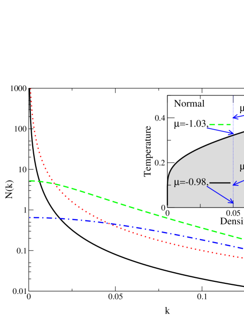
Figure 3: Momentum distribution of photons, from which follows the angular distribution. Two uncondensed, and two condensed distribution are shown, for mean field densities as shown in the inset. (Parameters $\Delta^{\ast}=0$, $m^{\ast}=0.01$.)

We now estimate the phase boundary including the effects of fluctuations. We calculate the free energy from the action in eq. (3), evaluated to Gaussian order. Taking the total derivative of free energy w.r.t. chemical potential gives the total density, and evaluating this at the critical chemical potential gives an estimate of the phase boundary. This follows the method of Nozières and Schmitt-Rink (1985), but is complicated by the effects of a dynamic boson field and by two-dimensionality.

The total density is

$$\rho = \frac{n}{2}\left(1-\frac{\tilde{\epsilon}}{E}\tanh(\beta E)\right)+\frac{\left|\psi_{0}\right|^{2}}{A}$$ (12)

$$+ \int_{0}^{K}(dk)^{2}\left(f(\xi_{1})+f(\xi_{2})-f(2E)+g(k)\right)$$

when condensed, with $f(x)=-(n_{B}(x)+1/2)dx/d\mu$, and $g(k)$ due to $\delta\omega$; and

$$\rho=\frac{n}{1+e^{2\beta\tilde{\epsilon}}}+\int_{0}^{K}(dk)^{2}\left(f(E_{+})+f(E_{-})-f(2\tilde{\epsilon})\right)$$ (13)

with $f(x)=-n_{B}(x)dx/d\mu$ when uncondensed.

Considering the terms in eq. (12), these can be identified as exciton density and coherent photon density on the first line. Under the integral are the occupation of upper and lower polaritons, and subtraction of exciton density, required as excitons would otherwise be counted twice. The cutoff $K$ regularises the ultraviolet divergence. The theory is not renormalisable, due to the constant coupling between high energy photon modes and the excitons; but for low energy properties, changing the cutoff introduces only small corrections.

However, as well as changing density, fluctuations change the critical chemical potential by depleting the condensatePopov (1983). Therefore, it is necessary to make a separate estimate of the condensate density including fluctuations. For a two dimensional system, this can be achieved by calculating the superfluid response, which requires comparing the transverse (normal) response, and the total density:

$$\rho_{s} = \rho_{p}-\rho_{n},\quad\rho_{n}=\frac{1}{m\beta A}\lim_{q\rightarrow 0}\left[\left(\delta_{ij}-\frac{q_{i}q_{j}}{q^{2}}\right)\chi_{ij}(q)\right]$$

$$\chi_{ij}(q) = \mathrm{Tr}\left(\frac{k_{i}k_{j}}{2}\mathcal{G}\left(\omega,k-\frac{q}{2}\right)\sigma_{3}\mathcal{G}\left(\omega,k+\frac{q}{2}\right)\sigma_{3}\right)$$ (14)

where $\mathcal{G}$ is the photon greens function, and $\rho_{p}$ is the total photon density. The transverse response may be safely calculated without vertex corrections, as these affect only the longitudinal response. Combining the results of eq. (12) and eq. (Polariton condensation with localised excitons and propagating photons), the phase transition including fluctuations occurs when $\rho_{s}=0$. As the system is two dimensional, one ought to consider a Kosterlitz-Thouless transition, at finite $\rho_{s}$, but this introduces only small corrections. The phase boundaries for four different photon masses are shown in figure 4.

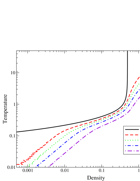
Figure 4: Phase boundaries calculated from mean field theory, and including fluctuation corrections for four different values of photon mass. Temperature and density plotted in units of $g\sqrt{n}$ and $n$.

At low densities, the phase transition occurs as the condensate is depleted by occupation of the phase mode. Therefore, the phase boundary has the form $T_{c}\propto\rho/m_{\mathrm{pol}}$ where $m_{\mathrm{pol}}$ is the polariton mass, which, at resonance, is just $2m$. This compares to the mean field boundary, which at resonance is

$$T_{c}=g\sqrt{n}\frac{\sqrt{1-2\rho}}{2\tanh^{-1}(1-2\rho)}\approx\frac{g\sqrt{n}}{-\ln\rho},$$ (15)

the second equality being valid for small densities. This temperature is effectively constant on the scale of the B.E.C. phase boundary.

As the density increases, the phase boundary including fluctuations will approach the mean field boundary. Due to the slow dependence of the mean field boundary on density, this will occur at $T\approx g\sqrt{n}$, unless mass is very large. The exact temperature where this occurs depends on the mass. For a small mass the fluctuation boundary follows the mean field boundary over a wider range of densities. The rescaled photon mass, $m^{\ast}$, provides a small parameter near $T\approx g\sqrt{n}$, $\rho\approx n$. Physically, at a temperature scale of $g\sqrt{n}$, the fluctuation modes are occupied to the top of the lower polariton branch, and occupation of the upper branch becomes relevant.

At yet higher densities, the fluctuation result again differs from the mean field. For $\rho>n$ the mean field theory will always predict a condensate. However, at high densities, the system is dominated by incoherent photons, not described in the mean field theory. In this limit the phase boundary is that for B.E.C. of (massive) photons.

To conclude, we have calculated the spectrum of fluctuations for a model of localised excitons interacting with propagating photons. In the condensed state, the fluctuations about mean field include the Goldstone mode, and the linear dispersion causes a characteristic change to the momentum distribution of photons. Both the narrowing of the $N(k)$ distribution and the gap between coherent and incoherent luminescence would provide evidence for polariton condensation. Fluctuations alter the form of the phase transition. At low densities the transition has the $T_{c}\propto\rho$ form expected for Bose condensation of pre-formed Bosons. As the density increases, for small masses, the mean field interaction driven limit is recovered, for densities $\rho\approx n$. However, for yet higher densities, the boundary changes again, to Bose condensation of weakly interacting photons.

We are grateful to B. D. Simons for useful discussions, and for support from the Cambridge-MIT Institute (JK), Sidney Sussex college, Cambridge (PRE), Gonville and Caius College Cambridge (MHS) and the EU Network HPRN-CT-2002-00298.

References

- Dang et al. (1998) L. S. Dang, D. Heger, R. André, F. Bœuf, and R. Romestain, Phys. Rev. Lett. 81, 3920 (1998).
- Deng et al. (2002) H. Deng, G. Weihs, C. Santori, J. Bloch, and Y. Yamamoto, Science 298, 199 (2002).
- Deng et al. (2003) H. Deng, G. Weihs, D. Snoke, J. Bloch, and Y. Yamamoto, P.N.A.S. 100, 15318 (2003).
- Savvidis et al. (2000) P. G. Savvidis, J. J. Baumberg, R. M. Stevenson, M. S. Skolnick, D. M. Whittaker, and J. S. Roberts, Phys. Rev. Lett. 84, 1547 (2000).
- Kavokin et al. (2003) A. Kavokin, G. Malpuech, and F. P. Laussy, Phys. Lett. A 306, 187 (2003).
- Eastham and Littlewood (2001) P. R. Eastham and P. B. Littlewood, Phys. Rev. B 64, 235101 (2001).
- Lidzey et al. (1999,) D. G. Lidzey et al., Phys. Rev. Lett. 82, 3316 (1999).
- Woggon et al. (2003) U. Woggon et al., Appl. Phys. B-Lasers Opt. 77, 469 (2003).
- Hess et al. (1994) H. F. Hess, E. Betzig, T. D. Harris, L. N. Pfeiffer, and K. W. West, Science p. 1740 (1994).
- Szymanska et al. (2003) M. H. Szymanska, P. B. Littlewood, and B. D. Simons, Phys. Rev. A 68, 013818 (2003).
- Dicke (1954) R. H. Dicke, Phys. Rev. 93, 99 (1954).
- Hepp and Lieb (1973) K. Hepp and E. Lieb, Phys. Rev. A 8, 2517 (1973).
- Keeling et al. (2004) J. Keeling, L. S. Levitov, and P. B. Littlewood, Phys. Rev. Lett. 92, 176402 (2004).
- Nozières and Schmitt-Rink (1985) P. Nozières and S. Schmitt-Rink, J. LTP 59, 195 (1985).
- Popov (1983) V. N. Popov, Functional Integrals in Quantum Field Theory and Statistical Physics (D. Reidel, 1983), chap. 6.