Dynamics of a single ring of vortices in two-dimensional trapped Bose-Einstein condensates

Abstract

The dynamics of a ring of vortices in two-dimensional Bose-Einstein condensates (with and without an additional vortex at the center) is studied for (1) a uniform condensate in a rigid cylinder and (2) a nonuniform trapped condensate in the Thomas-Fermi limit. The sequence of ground states (within these single-ring configurations) is determined as a function of the external rotation frequency by comparing the free energy of the various states. For each ground state, the Tkachenko-like excitations and the associated dynamical stability are analyzed.

I introduction

The dynamics of quantized vortices has attracted great interest. Until recently most research has been done in the context of superfluid ⁴He Donn91 . The physics of an unbounded superfluid with an infinite number of vortices is relatively simple: In equilibrium the vortices form a two-dimensional rotating triangular vortex lattice, which supports small-amplitude collective modes Tkac66 . In a bounded superfluid, however, determining the equilibrium configuration is not easy even for a small number of vortices.

Havelock Have31 studied the dynamical stability of a ring with a small number of vortices. Subsequently, Hess Hess67 studied the energy of various configurations analytically to determine the sequence of low-lying equilibrium states, and Campbell and Ziff Camp79 evaluated the energies numerically for larger numbers of vortices. After heroic efforts, Yarmchuk et al. Pack79 photographed some stable vortex patterns in superfluid ⁴He.

For a large number of vortices, Fetter developed a theory of the dynamics of a lattice of slightly displaced rectilinear vortices Fett67 including three-dimensional distortions. Later, the description was extended to provide a continuum picture of the vortex dynamics Fett77 . Baym and Chandler formulated similar macroscopic hydrodynamics of rotating superfluids Baym83 . These various theoretical descriptions included the vortex-interaction effects discussed by Tkachenko Tkac66 . For a comprehensive review of vortex dynamics in rotating superfluids, see, for example, Ref. Soni87 .

The strong interaction between helium atoms makes it difficult to manipulate the condensate and to observe vortices. Thus, the detection of quantized vortices in trapped Bose-Einstein condensates Matt99 ; Dali00 ; Madi00 offers an opportunity to study the dynamics of superfluid vortices. In addition, the interaction parameter is tunable by varying the number of atoms, which helps clarify their many-body character and the detailed connection to fluid dynamics. Recent experiments at JILA Codd03 measured the transverse elastic modes of the bounded vortex lattice that have been studied theoretically by Angl02 ; Baym03 ; Stri04 ; Soni04 . These Tkachenko modes Tkac66 in a large but finite lattice require appropriate and nontrivial boundary conditions.

Here, we study the equilibrium states and small oscillations of (1) a ring of $N_{v}$ vortices and (2) a ring of $N_{v}-1$ vortices plus a central vortex for two specific cases: a cylindrical container with uniform fluid and a two-dimensional condensate in a harmonic radial trap in the Thomas-Fermi (TF) limit. These vortex states can be stable up to $N_{v}\sim 9$, beyond which other more complicated configurations become favorable. The associated normal modes are small-system analogs of the Tkachenko modes for a large vortex array.

II time-dependent variational formalism

A macroscopic order parameter (the condensate wave function) $\Psi\equiv\langle\hat{\Psi}\rangle$, with associated particle density $n=\left|\Psi\right|^{2}$, provides a simple description of a Bose-Einstein condensate near $T=0$ K. In the presence of an external trap potential $V_{\mathrm{tr}}$, the condensate experiences both $V_{\mathrm{tr}}$ and the self-consistent Hartree interaction $V_{\mathrm{H}}=g|\Psi|^{2}=gn$ arising from the interaction with all other particles, where $g=4\pi\hbar^{2}a_{s}/M$ is the interparticle interaction parameter (assumed to be repulsive) and $a_{s}$ is the positive $s$-wave scattering length Dalf99 ; Fett99 .

At zero temperature in the laboratory (nonrotating) frame, the macroscopic order parameter $\Psi$ satisfies the time-dependent, nonlinear Schrödinger equation (Gross-Pitaevskii equation),

$$i\hbar\frac{\partial\Psi}{\partial t}=-\frac{\hbar^{2}\nabla^{2}}{2M}\Psi+V_{\mathrm{tr}}\Psi+g\left|\Psi\right|^{2}\Psi.$$ (1)

If the external potential rotates at an angular velocity $\bm{\Omega}$, it is necessary to transform to a co-rotating frame, in which case the time-dependent Schrödinger equation becomes Landau

$$i\hbar\frac{\partial\Psi}{\partial t}=-\frac{\hbar^{2}\nabla^{2}}{2M}\Psi+V_{\mathrm{tr}}\Psi-\bm{\Omega}\cdot\mathbf{r}\times\mathbf{p}\,\Psi+g\left|\Psi\right|^{2}\Psi,$$ (2)

where $\mathbf{r}\times\mathbf{p}=-i\hbar\mathbf{r}\times\bm{\nabla}$ is the angular-momentum operator.

For many purposes, however, it is more convenient to use an equivalent Lagrangian formalism based on the Lagrangian functional Pere96 ,

$$\mathcal{L}[\Psi]\equiv\mathcal{T}[\Psi]-\mathcal{E}^{\prime}[\Psi].$$ (3)

Here

$$\mathcal{T}[\Psi]=\int dV\,\frac{i\hbar}{2}\left(\Psi^{*}\frac{\partial\Psi}{\partial t}-\frac{\partial\Psi^{*}}{\partial t}\Psi\right),$$ (4)

is the time-dependent part of the Lagrangian, the analog of the kinetic energy in classical mechanics. In a nonrotating frame, $\mathcal{E}[\Psi]$ is the energy functional. In the reference frame that rotates at the same angular velocity $\mathbf{\Omega}$ as the external trap potential, the appropriate free energy functional acquires an additional term, $\mathcal{E}^{\prime}[\Psi]=\mathcal{E}[\Psi]-\mathbf{\Omega}\cdot\mathbf{L}[\Psi]$, where $\mathbf{L}[\Psi]$ is the angular momentum of the condensate. When $\bm{\Omega}=\Omega\hat{\mathbf{z}}$ is oriented along $\hat{\mathbf{z}}$, $\mathcal{E}^{\prime}$ can be written as

$$\mathcal{E}^{\prime}[\Psi]=\int dV\left(\frac{\hbar^{2}}{2M}\left|\bm{\nabla}\Psi\right|^{2}+V_{\mathrm{tr}}\left|\Psi\right|^{2}+\frac{g}{2}\left|\Psi\right|^{4}+i\hbar\Omega\Psi^{*}\frac{\partial\Psi}{\partial\phi}\right).$$ (5)

The action $\mathcal{S}$ associated with the above Lagrangian is the time integral $\mathcal{S}[\Psi]=\int dt~{}\mathcal{L}[\Psi]$. It is stationary with respect to small variations of $\Psi$ and $\Psi^{*}$, when $\Psi$ satisfies the time-dependent Gross-Pitaevskii (GP) equation (2). Thus the time-dependent GP equation is the Euler-Lagrange equation for the Lagrangian functional.

This Lagrangian formalism has the following significant advantage: not only is this approach exact, but also it provides the basis for a powerful approximate variational method. If the condensate wave function depends on various parameters $\{\mathbf{p}\}$ of the given system, the resulting Lagrangian $\mathcal{L}(\{\mathbf{p}\})$ provides the dynamical equations of motion of these parameters $\{\mathbf{p}\}$. Moreover, when the system under consideration is in equilibrium and the variational parameters of the problem are stationary, the next-order perturbation (variation) of the Lagrangian yields the normal modes of the system in terms of these parameters.

Here we use this method to study the dynamics of vortices in a ring in a two-dimensional Bose condensate. The positions of the vortices {$\mathbf{r}_{j}$} serve as the time-dependent variational parameters for two distinct cases: (1) a uniform condensate in a rigid cylinder and (2) a nonuniform trapped condensate in the TF limit Baym96 .

In our variational approach, we use a trial wave function of the following form

$$\Psi(\mathbf{r},\{\mathbf{r}_{j}\})=\left|\Psi(\mathbf{r})\right|e^{iS(\mathbf{r},\{\mathbf{r}_{j}\})},$$ (6)

where $\left|\Psi\right|^{2}$ is the density profile of either the uniform condensate or the nonuniform TF condensate. It satisfies the normalization condition

$$N=\int dV\left|\Psi\right|^{2},$$ (7)

where $N$ is the number of condensate particles. In addition, $S(\mathbf{r},\{\mathbf{r}_{j}\})$ is the phase of the condensate wave function, and the particle velocity field is given by $\mathbf{v}(\mathbf{r})=\left(\hbar/M\right)\bm{\nabla}S(\mathbf{r})$. The trial wave function (6) assumes that the vortices do not affect the density profile of the condensate (this approximation holds for small cores, which is valid in the TF limit); instead, the vortices directly determine the velocity field. For simplicity, we consider only a condensate in two dimensions, when the various terms in the Lagrangian are interpreted per unit length.

III free energy and equilibrium states

To proceed, it is first necessary to choose a specific form for the phase $S$ of the condensate wave function. The boundary conditions are quite different for a uniform condensate and for a TF condensate, and it is convenient to treat them separately.

III.1 Uniform condensate in a cylinder

The uniform condensate in a rigid circular cylinder of radius $R$ must satisfy the boundary condition that the normal component of the particle current vanishes at the surface of the cylinder. This condition can be ensured with an image vortex of opposite circulation at the external position $\mathbf{r}_{j}^{\prime}=\left(R^{2}/r^{2}_{j}\right)\mathbf{r}_{j}$ for each vortex at $\mathbf{r}_{j}$ in the cylinder.

The time-dependent part $\mathcal{T}$ of the Lagrangian can be easily evaluated. The trial condensate wave function is

$$\Psi(\mathbf{r},\{\mathbf{r}_{j}\})=\sqrt{n}e^{iS(\mathbf{r},\{\mathbf{r}_{j}\})},$$ (8)

and

$$S(\mathbf{r},\{\mathbf{r}_{j}\})=\sum_{j=1}^{N_{v}}S_{j}(\mathbf{r},\mathbf{r}_{j})+\sum_{j=1}^{N_{v}}S_{j}^{\prime}(\mathbf{r},\mathbf{r}_{j}^{\prime}),$$ (9)

where

$$S_{j}(\mathbf{r},\mathbf{r}_{j}) =\arctan\left(\frac{y-y_{j}}{x-x_{j}}\right),$$ (10)

$$S_{j}^{\prime}(\mathbf{r},\mathbf{r}_{j}^{\prime}) =(-1)\arctan\left(\frac{y-y_{j}^{\prime}}{x-x_{j}^{\prime}}\right),$$ (11)

$n=N/V$ is the particle density and $N_{v}$ is the number of the vortices in the condensate. In cylindrical coordinates, we obtain

$$\mathcal{T}(\{\mathbf{r}_{j}\})=\sum_{j=1}^{N_{v}}\mathcal{T}_{j}(\mathbf{r}_{j})=\sum_{j=1}^{N_{v}}\left(1-r_{j}^{2}\right)\dot{\phi}_{j},$$ (12)

where each quantity is per particle and written in dimensionless units: the length scaled by the radius of the cylinder $R$, the time scaled by $\Omega_{0}^{-1}\equiv MR^{2}/\hbar$ and the energy by $\hbar\Omega_{0}$.

In the free energy part of the Lagrangian, the quantity of interest is the difference $\Delta\mathcal{E}^{\prime}$ of the free energy between the vortex state and the vortex-free state. In our approximation, this difference arises from the superfluid velocity field $\mathbf{v}$ caused by the presence of the vortices. It can be simply determined as

$$\Delta\mathcal{E}^{\prime}=\Delta\mathcal{E}-\Omega L_{z},$$ (13)

where $\Delta\mathcal{E}$ is the contribution from the superfluid velocity field in the nonrotating reference frame

$$\Delta\mathcal{E}=\int d^{2}\mathbf{r}\left|\Psi\right|^{2}\frac{1}{2}\,\mathbf{v}^{2},$$ (14)

and $L_{z}$ is the $z$ component of the angular momentum

$$L_{z}=\int d^{2}\mathbf{r}\left|\Psi\right|^{2}\hat{\mathbf{z}}\cdot\mathbf{r}\times\mathbf{v}.$$ (15)

In evaluating the free energy part, it is convenient to use a stream function $\chi$ instead of the phase of the condensate wave function $S$ (which is effectively a velocity potential). Thus, we choose

$$\chi(\mathbf{r},\{\mathbf{r}_{j}\})=\sum_{j=1}^{N_{v}}\chi_{j}(\mathbf{r},\mathbf{r}_{j})+\sum_{j=1}^{N_{v}}\chi_{j}^{\prime}(\mathbf{r},\mathbf{r}_{j}^{\prime}),$$ (16)

where

$$\chi_{j}(\mathbf{r},\mathbf{r}_{j}) =\ln\left|\mathbf{r}-\mathbf{r}_{j}\right|,$$ (17)

$$\chi^{\prime}_{j}(\mathbf{r},\mathbf{r}_{j}^{\prime}) =(-1)\ln\left|\mathbf{r}-\mathbf{r}_{j}^{\prime}\right|,$$ (18)

and the velocity field is given by

$$\mathbf{v}(\mathbf{r})=\hat{\mathbf{z}}\times\bm{\nabla}\chi.$$ (19)

This two-dimensional stream function has the advantage being single-valued. When describing irrotational flow in the presence of vortices, $\chi$ satisfies Poisson’s equation

$$\nabla^{2}\chi(\mathbf{r},\{\mathbf{r}_{j}\})=2\pi\sum_{j=1}^{N_{v}}\delta^{(2)}\left(\mathbf{r}-\mathbf{r}_{j}\right).$$ (20)

The right-hand side vanishes everywhere except for the finite number of singular points at the location of the vortices (the image vortices lie outside the physical region and do not appear here). Thus, this stream function is essentially a superposition of two-dimensional Green’s functions.

Each individual term $\chi_{j}(\mathbf{r},\mathbf{r}_{j})$ has the Fourier expansion,

$$\chi_{j}(\mathbf{r},\mathbf{r}_{j})=\Theta(r-r_{j})\left[\ln r-\sum_{m=1}^{\infty}\frac{\cos m\phi}{m}\left(\frac{r_{j}}{r}\right)^{m}\right]+\Theta(r_{j}-r)\left[\ln r_{j}-\sum_{m=1}^{\infty}\frac{\cos m\phi}{m}\left(\frac{r}{r_{j}}\right)^{m}\right],$$ (21)

where

$$\Theta(r-r_{j})=\begin{cases}1,\qquad\text{if}~{}~{}r>r_{j},\\ 0,\qquad\text{if}~{}~{}r<r_{j},\end{cases}$$ (22)

is the unit positive step function and $\phi$ is the angle between $\mathbf{r}$ and $\mathbf{r}_{j}$. Straightforward analysis then yields the free energy difference Hess67 ,

$$\begin{split}\Delta\mathcal{E}^{\prime}(\{\mathbf{r}_{j}\})=&N_{v}\ln\left(\frac{R}{\xi}\right)+\sum_{j=1}^{N_{v}}\ln\left(1-r_{j}^{2}\right)-\Omega\sum_{j=1}^{N_{v}}\left(1-r_{j}^{2}\right)\\ &\phantom{~{}}+\sum_{i<j}^{N_{v}}\ln\left(\frac{1-2r_{i}r_{j}\cos\phi_{ij}+r_{i}^{2}r_{j}^{2}}{r_{i}^{2}-2r_{i}r_{j}\cos\phi_{ij}+r_{j}^{2}}\right),\end{split}$$ (23)

where $\xi$ is the healing length of the condensate (the vortex-core-radius cutoff) and $\phi_{ij}\equiv\phi_{i}-\phi_{j}$ is the angle between the $i$th and the $j$th vortices. Each vortex interacts with all other vortices including images, as is evident from the last term. Note that $\Omega$ is also written in dimensionless units scaled with $\Omega_{0}$.

III.2 TF condensate

In the TF limit, it is more convenient to work with the equivalent grand canonical ensemble, introducing the chemical potential $\mu$ that is determined by the normalization condition $N=\int dV\left|\Psi\right|^{2}$. Then the condensate wave function gives the following TF density profile

$$\left|\Psi(\mathbf{r})\right|^{2}=n_{0}\left(1-r^{2}\right),$$ (24)

where $n_{0}=\mu/g$ is the central density and $r$ is a dimensionless radius, scaled by the TF radius $R=\sqrt{2\mu/M\omega_{\perp}^{2}}$ (in the TF limit, $\mu\gg\hbar\omega_{\perp}$, which implies that $R$ is large compared to the oscillator length $\sqrt{\hbar/M\omega_{\perp}}$).

In the TF case, the condensate density vanishes at the boundary ($r=1$). Thus the particle current automatically satisfies the boundary condition, and image vortices are unnecessary. When the energy is scaled by the characteristic energy $\hbar\Omega_{0}=\hbar^{2}/MR^{2}=(\hbar\omega_{\perp}/2\mu)\,\hbar\omega_{\perp}$, the time-dependent part of the Lagrangian per particle is

$$\mathcal{T}(\{\mathbf{r}_{j}\})=\sum_{j=1}^{N_{v}}\mathcal{T}_{j}(\mathbf{r}_{j})=-\sum_{j=1}^{N_{v}}\left(r_{j}^{2}-\frac{r_{j}^{4}}{2}\right)\dot{\phi}_{j}.$$ (25)

The free energy difference per particle can be evaluated using the same Fourier expansion (21) for the stream functions (see Appendix A), which yields

$$\begin{split}\Delta\mathcal{E}^{\prime}(\{\mathbf{r}_{j}\})&=\frac{1}{2}\sum_{j=1}^{N_{v}}\left\{\left(1-r_{j}^{2}\right)\left[2\ln\left(\frac{R}{\xi}\right)+\ln\left(1-r_{j}^{2}\right)\right]+\left(2r_{j}^{2}-1\right)-\Omega\left(1-r_{j}^{2}\right)^{2}\right\}\\ &\phantom{=~{}~{}}+\frac{1}{2}\sum_{i<j}^{N_{v}}\left(1-r_{i}r_{j}\cos\phi_{ij}\right)\ln\left[\frac{1-2r_{i}r_{j}\cos\phi_{ij}+r_{i}^{2}r_{j}^{2}}{\left(r_{i}^{2}-2r_{i}r_{j}\cos\phi_{ij}+r_{j}^{2}\right)^{2}}\right]\\ &\phantom{=~{}~{}}+\sum_{i<j}^{N_{v}}r_{i}r_{j}\sin\phi_{ij}\arctan\left(\frac{-r_{i}r_{j}\sin\phi_{ij}}{1-r_{i}r_{j}\cos\phi_{ij}}\right)\\ &\phantom{=~{}~{}}-\sum_{i<j}^{N_{v}}\left(1-r_{i}^{2}-r_{j}^{2}\right).\end{split}$$ (26)

III.3 Euler-Lagrange equations of motion

The Euler-Lagrange equations for the Lagrangian $\mathcal{L}=\mathcal{T}-\mathcal{E}^{\prime}$ are

$$0 =\frac{d}{dt}\frac{\partial\mathcal{L}}{\partial\dot{r}_{j}}-\frac{\partial\mathcal{L}}{\partial r_{j}},$$ (27)

$$0 =\frac{d}{dt}\frac{\partial\mathcal{L}}{\partial\dot{\phi}_{j}}-\frac{\partial\mathcal{L}}{\partial\phi_{j}}.$$ (28)

Since $\mathcal{L}$ is independent of $\dot{r}_{j}$ for the configurations studied here, the first equation reduces to $\partial\mathcal{L}/\partial r_{j}=0$, which determines the precession frequency of the $j$th vortex [see Eqs. (12) and (25)],

$$\dot{\phi}_{j}=\left(\frac{\partial\Delta\mathcal{E}^{\prime}}{\partial r_{j}}\right)\Bigg{/}\left(\frac{1}{\dot{\phi}_{j}}\,\frac{\partial\mathcal{T}}{\partial r_{j}}\right).$$ (29)

If the system is nondissipative and all vortices lie symmetrically spaced on a single ring of radius $r$, they are locked together and precess at the same rate $\dot{\phi}=\dot{\phi}_{j}(r,\Omega)$.

III.4 Uniform precession of a single vortex

It is interesting to start with the simplest case of a single vortex, which clarifies the distinct role of the factor $\ln\left(R/\xi\right)$ between the Lagrangians for the uniform condensate and the TF condensate. Consider the uniform condensate, where the free energy part of the Lagrangian (23) contains the logarithm $\ln\left(R/\xi\right)$ only as an additive constant $N_{v}\ln\left(R/\xi\right)$, independent of the coordinates of the vortices. Thus, this logarithmic factor $\ln\left(R/\xi\right)$ affects the energy-related properties, such as the ground-state configuration and the angular velocity for transitions between adjacent states; in contrast, the same factor does not affect either the radius of the ring of vortices or the precession frequency. For example, Eq. (29) gives the scaled precession frequency for a single vortex at a distance $r_{1}$ in a uniform nonrotating condensate

$$\dot{\phi}_{1}=\frac{1}{1-r_{1}^{2}}.$$ (30)

From a physical viewpoint, the single vortex in a uniform condensate precesses under the influence of its opposite image vortex, which explains why the precession rate increases as the vortex moves toward the outer boundary.

An expansion of $\Delta\mathcal{E}^{\prime}(r_{1})$ from Eq. (23) for small $r_{1}$ near the center of the condensate shows that the curvature changes sign at $\Omega_{m}=1$. This value is the same as the precession frequency for a nearly central vortex in a nonrotating condensate; $\Omega_{m}$ corresponds to the onset of metastability for a central vortex Pack72 .

The situation is quite different for the TF condensate, where Eq. (26) has $\ln\left(R/\xi\right)$ in a term that depends on the coordinates of the vortices. Use of Eq. (29) readily yields the corresponding TF precession frequency for a single vortex at $r_{1}$ in a nonrotating condensate

$$\dot{\phi}_{1}=\frac{1}{1-r_{1}^{2}}\left[\ln\left(\frac{R}{\xi}\right)+\frac{1}{2}\ln(1-r_{1}^{2})-\frac{1}{2}\right].$$ (31)

Equation (31) differs from Eq. (30) because of the “large” factor $\ln\left(R/\xi\right)$, which arises from the radial derivative of the energy in the numerator of Eq. (29). Although both (30) and (31) have similar denominators, the present factor $\left(1-r_{1}^{2}\right)^{-1}$ reflects the nonuniform TF density Jack99 ; Lund00 ; McGee01 ; Fett01 (instead of the image, since the TF condensate has no image vortices). Physically, the precession here arises from the combination of the Magnus force and the gradient in the density (or equivalently the trap potential in this TF limit) Svid00 ; Svid00a ; Shee04 .

An expansion of $\Delta\mathcal{E}^{\prime}(r_{1})$ from Eq. (26) for small $r_{1}$ near the center of the condensate shows that the curvature now changes sign at $\Omega_{m}=\ln(R/\xi)-\frac{1}{2}$, which is again the same as the precession frequency for a nearly central vortex in a nonrotating condensate. This value also corresponds to the onset of metastability, now enhanced by the large logarithmic factor.

III.5 State of lowest free energy

In the presence of any small dissipative process, the system seeks the state of lowest free energy for a given external rotation by adjusting the radius of the ring of vortices to be $r_{r}$, determined by the condition

$$0=\left.\frac{\partial\Delta\mathcal{E}^{\prime}}{\partial r_{j}}\right|_{\{r_{j}\}=r_{r}}.$$ (32)

In this case, Eq. (29) shows that $\dot{\phi}=0$, which means that the position of each vortex does not change. Hence all vortices are stationary in the co-rotating reference frame. In the laboratory (inertial) frame, the vortices all rotate at the same rate as the external rotation $\Omega$. Physically this result can be understood when we imagine that the vortex core contains some normal component, and the relative motion of the normal component with respect to the frame of the rotating trap gives rise to dissipation.

This equilibrium radius $r_{r}$ is a function of the external rotation $\Omega$. For a given vortex configuration, we can evaluate the lowest free energy $\Delta\mathcal{E}^{\prime}_{\mathrm{min}}(r_{r},\Omega)$ by solving Eq. (32). Comparing these lowest free energies among the different vortex states, we can determine the state with lowest energy and the associated angular velocity $\Omega_{c}^{AB}$, at which the transition from vortex state $A$ to vortex state $B$ should occur. Here we will consider two types of vortex configurations for each (uniform/TF) condensate; a ring of vortices without a vortex at the center (‘$N_{r}$’ configuration) and a ring of vortices with a vortex at the center (‘$N_{r}$+①’ configuration).

For both the uniform and the TF condensates, the vortex-free state is energetically favored for any angular velocity below $\Omega_{c}^{01}$ because it has the lowest free energy. As $\Omega$ increases, however, the free energy of the one-vortex state decreases at a faster rate than that of the vortex-free state. At $\Omega_{c}^{01}$, the free energy of the two states is the same, and the condensate can support a central vortex throughout the interval $\Omega_{c}^{01}\leq\Omega\leq\Omega_{c}^{12}$. At higher $\Omega$ between $\Omega_{c}^{12}$ and $\Omega_{c}^{23}$, the state with two vortices has the lowest energy, and so on.

The two condensates display one interesting difference, however, arising from the different density profiles. In the TF approximation, the thermodynamic critical angular velocity $\Omega_{c}^{01}$ (the usual lower critical angular velocity $\Omega_{c1}$) for the appearance of the first central vortex is given very generally by

$$\Omega_{c}^{01}=\frac{\Delta\mathcal{E}_{1}}{L_{1}}=\frac{\int d^{2}r\,\frac{1}{2}v^{2}n(r)}{\int d^{2}r\,n(r)}=\frac{1}{2}\frac{\int d^{2}r\,r^{-2}n(r)}{\int d^{2}r\,n(r)},$$ (33)

where $\Delta\mathcal{E}_{1}$ is the energy per particle for one central vortex and $L_{1}$ is the angular momentum per particle for the same central vortex. Evidently, $\Omega_{c}^{01}$ is proportional to the average value of $r^{-2}$ with the number density as the non-negative weight. The TF condensate $n_{TF}(r)\propto 1-r^{2}$ has the maximum density at the center; thus the corresponding $\Omega_{c}^{01}$ is larger than that for the uniform condensate (the difference leads to a factor $\approx 2$ in the present two-dimensional case).

The state with five vortices in a ring plus one at the center (5+① configuration) always has a lower free energy than the state with all six vortices in a ring (6 configuration), so the ‘5’ to ‘6’ transition is not favored; instead, ‘5’ goes to ‘5+①’. In fact, this specific ‘5’ to ‘5+①’ transition was observed in an early experiment on rotating superfluid ⁴He Pack79 . In a uniform unbounded condensate, the vortices form a triangular (Abrikosov) lattice with six-fold rotational symmetry. Here the transition from a single ring with an empty center (‘$N_{r}$’) to a ring with a central vortex (‘$N_{r}$+①’) happens when the condensate has five vortices in a ring ($N_{r}=5$) instead of six, which reflects the finite size of our geometry.

(a) uniform condensate	(b) TF condensate

Figure 1: Angular momentum per vortex as a function of the external rotation. Here, we assume $\ln\left(R/\xi\right)=8$.

It is interesting to consider the angular momentum per particle $L_{z}$, which follows directly from the thermodynamic relation

$$L_{z}=-\left(\frac{\partial\mathcal{E}^{\prime}}{\partial\Omega}\right)_{\mathrm{eq}}.$$ (34)

As a function of $\Omega$, the envelope of the minimum free energy curves is approximately proportional to $-\Omega^{2}$, apart from small irregularities associated with the small number of vortices, so that $L_{z}$ increases approximately linearly with $\Omega$. For a given vortex state, the angular momentum increases slowly with the external rotation as the radius of the ring of vortices shrinks to satisfy Eq. (32). Since the number of vortices also increases nearly linearly with $\Omega$, it is natural to consider the ratio $L_{z}/N_{v}$, which is the angular momentum (per particle) per vortex. This ratio $L_{z}/N_{v}$ is precisely 1 for a single central vortex. For many vortices, in contrast, the velocity approaches $\mathbf{\Omega}\times\mathbf{r}$ (solid-body rotation). In our dimensionless units, $L_{z}/N_{v}$ is then the average of $r^{2}$ weighted with the particle density $n(r)$, which is $\frac{1}{2}$ for a uniform condensate and $\frac{1}{3}$ for the TF condensate trapped in a harmonic potential. Thus the ratio $L_{z}/N_{v}$ should start at 1 for both condensates and decrease slowly toward the appropriate limit with increasing $\Omega$. This reduction of the angular momentum (per particle) per vortex from 1 was observed in Chev00 .

Figure 1 shows our calculated angular momentum (per particle) per vortex ($L_{z}/N_{v}$) as a function of the external rotation $\Omega$. As expected from the above estimate, the angular momentum per vortex of the TF condensate falls more rapidly (typically by $\sim 1.4-1.6\sim\frac{3}{2}$) as the number of vortices increases.

IV Tkachenko-like oscillation modes and the associated stability

Once we have an equilibrium ground state, we can consider small excitations of the ground state by considering small variations about the equilibrium. The in-plane, nearly transverse excitation modes of the infinite vortex lattice in the uniform Bose condensate are the well-known Tkachenko modes Tkac66 . Here we consider the finite-size analog of the Tkachenko modes both in the bounded uniform condensate and in the trapped TF condensate.

Let $\alpha_{j}$ and $\beta_{j}$ be the small variations of the radial distance and the angle, respectively, for the $j$th vortex in a ring,

$$r_{j}=r_{r}+\alpha_{j},\qquad\phi_{j}=\phi_{j}^{0}+\beta_{j},$$ (35)

where ($r_{r},\phi_{j}^{0}$) is the equilibrium position of the $j$th vortex. In equilibrium $N_{r}$ vortices are symmetrically placed in a ring: $N_{r}=N_{v}$ for a state without a vortex at the center and $N_{r}=N_{v}-1$ for a state with an extra vortex at the center; the state has a $N_{r}$-fold rotational symmetry. Thus a Fourier decomposition for $\bm{\alpha}$ and $\bm{\beta}$ will solve the problem:

$$\begin{pmatrix}\alpha_{j}\\ \beta_{j}\end{pmatrix}=\sum_{s=0}^{N_{r}-1}\begin{pmatrix}\tilde{\alpha}_{s}\\ \tilde{\beta}_{s}\end{pmatrix}e^{i2\pi js/N_{r}},$$ (36)

where the Fourier index $s$ runs from 0 to $N_{r}-1$.

The vortex at the center requires a special treatment. Since polar coordinates become singular at the origin, it is more convenient to use cartesian coordinates ($x$,$y$) for the vortex at the center, and polar coordinates ($r_{j}$,$\phi_{j}$) for the rest of the vortices in the ring. In this mixed-coordinate representation with $x$, $y$, $r_{j}$ and $\phi_{j}$, the Euler-Lagrange equations of motion for the small variations become

$$\frac{d}{dt}\mathbf{d}=T_{2}^{-1}GE_{2}\mathbf{d},$$ (37)

where $\mathbf{d}\equiv\left(x,y,\bm{\alpha},\bm{\beta}\right)$ is a vector. The matrix $T_{2}=\mathrm{diag}\left(2,2,t,\cdots,t,t,\cdots,t\right)$, with $t$ (it is independent of $q$) defined as

$$t\equiv\left(\frac{\partial^{2}\mathcal{T}}{\partial r_{q}\partial\dot{\phi}_{q}}\right)_{\mathrm{eq.}},$$ (38)

arises from the time-dependent part $\mathcal{T}$ of the Lagrangian. The matrix $E_{2}$ is the second-order expansion of the free energy part $\Delta\mathcal{E}^{\prime}$

$$\left(E_{2}\right)_{ij}=\left(\frac{\partial^{2}\Delta\mathcal{E}^{\prime}}{\partial D_{i}\partial D_{j}}\right)_{\mathrm{eq.}},$$ (39)

and here $\mathbf{D}\equiv\left(x,y,\mathbf{r},\bm{\phi}\right)$. The antisymmetric matrix $G$ shows how these small-variation parameters couple to form the dynamical structure of the system:

$$G=\begin{pmatrix}0&1&0&0\\ -1&0&0&0\\ 0&0&0&I_{N_{r}}\\ 0&0&-I_{N_{r}}&0\end{pmatrix},$$ (40)

where $I_{N_{r}}$ is the $N_{r}\times N_{r}$ identity matrix. To apply the above equation (37) to the condensate with no central vortex, ignore the first two components for $x$ and $y$ in $\mathbf{d}$ and set $x=y=0$ for the rest of the equations.

Although these equations look complicated, the Fourier decomposition (36) reduces them to a block-diagonal form, because $\Delta\mathcal{E}^{\prime}$ includes only two-body terms $\sim\int\mathbf{v}_{i}\cdot\mathbf{v}_{j}$ [see Eqs. (14), (23) and (26)]. When the Fourier components are projected out, the equations for $\tilde{\alpha}_{s}$ and $\tilde{\beta}_{s}$ simplify considerably. For $N_{r}=N_{v}-1$ vortices in a ring and one at the center, Eq. (36) and the orthogonality of the Fourier components decouple the original $2N_{v}\times 2N_{v}$ problem into one $6\times 6$ matrix problem,

$$\frac{d}{dt}\mathbf{P}_{6}=M_{6}\,\mathbf{P}_{6},$$ (41)

and $N_{r}-2$ sets of $2\times 2$ matrix problems ($s=0,2,\ldots,N_{r}-2$),

$$\frac{d}{dt}\mathbf{P}_{2}^{s}=M_{2}^{s}\,\mathbf{P}_{2}^{s},$$ (42)

where $\mathbf{P}_{6}=(x,y,\tilde{\alpha}_{1},\tilde{\alpha}_{N_{r}-1},\tilde{\beta}_{1},\tilde{\beta}_{N_{r}-1})$ and $\mathbf{P}_{2}^{s}=(\tilde{\alpha}_{s},\tilde{\beta}_{s})$ are 6- and 2-component vectors, respectively. If there is no vortex at the center, the original problem corresponds to $N_{r}=N_{v}$ sets of the above $2\times 2$ matrix problems [Eq. (42) with $s=0,1,\ldots,N_{r}-1$]. The matrix elements of $M_{6}$ and $M_{2}^{s}$ are determined from Eq. (37) (see Appendix B).

By solving these matrix problems, we can study the stability of the vortex system. For a given equilibrium state, we determine the excitation spectrum as a function of the external rotation frequency $\Omega$. If a particular excitation frequency is real, the corresponding small amplitudes ($x$,$y$,$\bm{\alpha}$,$\bm{\beta}$) oscillate around zero, and the state is stable. If any excitation frequency is complex with a positive imaginary part, the corresponding mode will grow with time, and the state is dynamically unstable.

(a) six vortices in a ring	(b) seven vortices in a ring

Figure 2: Imaginary parts of the excitation spectrum for a TF condensate showing the normal-mode index $s$ for each curve. Here, we assume $\ln\left(R/\xi\right)=8$.

As an example, Fig. 2 shows the positive imaginary parts of the excitation spectra for the system of six and seven vortices in a ring without a central vortex in the TF condensate. Since the complex excitation frequencies always appear in conjugate pairs, the figure shows only the positive imaginary parts. Above a critical angular velocity ($\sim 27.7$), a ring of six vortices becomes stable. In contrast, the ring of seven vortices is always unstable because a mode with positive imaginary part persists for any $\Omega$.

The Fourier index $s$ is analogous to the wave number in a linear array. For a given $N_{r}$, the normal modes become increasingly unstable as $s$ increases, so that the essential instability arises for short wave lengths. In the case of six vortices, $s=3$ (the mode with the shortest wave length) is the last mode to become stable. In the seven-vortex state, the shortest wave length modes are $s=(3~{}\text{or}~{}4)$, and these modes remain unstable for all angular velocity, indicating a “buckling” transition to a ‘6+①’ configuration, arising from the preference for a more uniform configuration.

IV.1 Uniform condensate

The dynamical instability of a finite number of vortices in a single ring without a central vortex was studied by Havelock Have31 . There, by solving the set of $2\times 2$ matrix problems (42), he concluded that a single ring is unstable when the number of vortices exceeds six. Here, we sharpen this result. Although six vortices in a ring are dynamically stable, we find that the configuration with ‘5+①’ has lower free energy compared to ‘6’.

Figure 3 (a) summarizes the conclusions of the free energy calculation and the stability analysis in a uniform condensate in a rigid cylinder. Here, the backslashed blocks show the regions where a given configuration has the lowest free energy. In the empty region to the left, there exist energetically more stable states with fewer vortices. For example, the empty region for the one-vortex state means that the vortex-free state is preferred to the one-vortex state. The slashed regions at the left side of the empty regions indicate the absence of a local free energy minimum. Hence, a state is metastable, but not globally stable, in the empty region (to the right of the slashed region). For each configuration, the narrow solid bar denotes the region where the particular array has at least one complex excitation frequency with a positive imaginary part (and is thus dynamically unstable).

Unlike the ring with no central vortex, the ring with a central vortex is stable even for a ring of eight vortices. The dynamical instability appears only for nine vortices in the ring with a central vortex, indicating the existence of other more stable states than this ‘9+①’ configuration. Campbell and Ziff Camp79 studied the stationary vortex patterns in a uniform condensate, evaluating the corresponding free energy for numbers of vortices $N_{v}=1$ to 30 (they did not investigate the small-amplitude normal modes). According to their findings, the stable state with the lowest free energy for a system of ten vortices, has ‘4+4+2’ vortices (three concentric rings; beginning from the outer-most ring); the ‘9+①’ configuration has slightly higher free energy and is nearly stable, as opposed to stable.

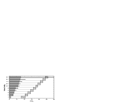
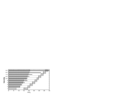
(a) uniform condensate	(b) TF condensate

Figure 3: Stability of single-ring states: backslashed blocks denote the region with lowest free energy; empty blocks denote metastable states that are local free energy minima but energetically disfavored because other more stable states exist; slashed blocks indicate regions where no local free energy minimum exists; the narrow solid bar denotes the region with complex excitation frequencies (and thus dynamically unstable). Here, we assume that $\ln\left(R/\xi\right)=8$.

IV.2 TF condensate

The TF condensate shows qualitatively the same behavior as the uniform condensate case, with small differences [see Fig. 3(b)].

1. For a single vortex, the dynamics is dominated either by the image vortex (for the uniform condensate) or by the nonuniform trap potential (for the TF condensate). For two or more vortices, however, the vortex-vortex interactions become increasingly dominant, and the two systems are expected to become more and more similar.

2. In a transition from ‘5’ to ‘5+①’ for the TF condensate, the region of complex excitation modes (indicated by the solid bar) remains almost unchanged, although the number of vortices increases.

3. Another notable difference is that, for the ‘8+①’ TF configuration, the region of complex eigenmodes (dynamically unstable) expands significantly, leaving a narrower region of external rotation frequency over which this configuration is metastable.

V discussion

The time-dependent variational analysis based on the Lagrangian formalism provides a direct and flexible method to study the dynamics of vortices in a Bose-Einstein condensate. By analyzing the time-independent free energy $\mathcal{E}^{\prime}$, we determine the various ground states and the associated angular velocities for the transitions from one state to the next. A more complete dynamical picture emerges when we consider the full Lagrangian $\mathcal{L}=\mathcal{T}-\mathcal{E}^{\prime}$, for it provides the explicit time dependence: for example, the vortex precession frequency, the excitation spectrum and the dynamical stability.

For a given configuration of vortices, the critical $\Omega$ for the onset of stability is larger for the TF condensate than for the uniform condensate, by approximately a factor of two. As a result, a single ring of $N_{r}$ vortices (without and with a central vortex) has a smaller radius in the TF condensate than in the uniform condensate, typically, by $\sim 0.9$.

The Lagrangian formalism has the notable feature that it apparently incorporates valuable physical information that would otherwise emerge only with significant additional effort. For example, the Lagrangian analysis of the low-lying normal modes of a condensate Pere96 used a Gaussian trial function, but the resulting dynamics reproduced the known frequencies even in the TF limit where the density profile has a parabolic form.

Similarly here, the Lagrangian formalism yields the correct precession of a single vortex, even though the assumed stream function is equivalent to purely incompressible flow. To understand this question in more detail, note that the velocity field assumed in Eq. (19) can equivalently be written as $\mathbf{v}=-\bm{\nabla}\times(\hat{\mathbf{z}}\chi)$, which implies that ${\bm{\nabla}\cdot\mathbf{v}}=0$. Since we are merely constructing a trial function, this choice is acceptable, even though the correct equation of continuity requires ${\bm{\nabla}\cdot(n\mathbf{v})}=0$. Nevertheless, the Lagrangian approach incorporates sufficient physical information (presumably through the energy $\mathcal{E}^{\prime}$) that the resulting precession in Eq. (31) agrees with other more lengthy analyses.

A direct approach to the precession relies on the full equation ${\bm{\nabla}\cdot(n\mathbf{v})}={\mathbf{v}}\cdot\bm{\nabla}n+n{\bm{\nabla}\cdot\mathbf{v}}=0$. The extra term involving $\bm{\nabla}n$ (namely the spatial variation in the condensate density) produces additional logarithmic contributions to the phase Svid00 ; Svid00a ; Shee04 , which drive the precessional motion. Thus the precession of a single vortex in a TF condensate can be considered to arise from the nonuniform trap potential and the resulting nonuniform TF density. It would be interesting to improve the trial function by including these additional logarithmic contributions explicitly. Since the variational Lagrangian approach is “exact” for the exact solution of the GP equation, such an improved wave function should provide an improved description, but it is not clear whether the dynamical precession rate would be affected.

As studied in this work, the single-ring configuration is applicable only for a small number of vortices ($N_{v}\lesssim 9$ in practice) in a TF condensate that rotates relatively slowly. The single ring does have one other very interesting application, however, when the condensate has a central hole and thus becomes annular. Such behavior is predicted to occur in a rapidly rotating trap with an additional quartic confinement, which allows the angular velocity $\Omega$ to exceed the harmonic trap frequency $\omega_{\perp}$. When the width of the annulus becomes sufficiently narrow, the condensate is predicted to have a one-dimensional array of vortices arranged in a single ring Kasa02 ; Fett04 . The techniques developed here should apply directly to the dynamics and stability of this interesting configuration.

Appendix A evaluating the TF free energy difference

With no loss of generality, consider the case with two vortices at $\mathbf{r}_{1}=(r_{1},\phi_{1})$ and $\mathbf{r}_{2}=(r_{2},\phi_{2})$. The stream function that describes the velocity field in the condensate is

$$\chi=\chi_{1}+\chi_{2}=\ln\left|\mathbf{r}-\mathbf{r}_{1}\right|+\ln\left|\mathbf{r}-\mathbf{r}_{2}\right|.$$ (43)

In the free energy difference $\Delta\mathcal{E}^{\prime}=\Delta\mathcal{E}-\Omega L_{z}$, the angular momentum is straightforward to evaluate and only $\Delta\mathcal{E}$ is of concern.

$$\begin{split}\Delta\mathcal{E}&=\frac{1}{2}\int d^{2}\mathbf{r}~{}n(r)\mathbf{v}^{2}\\ &=\frac{1}{2}\int d^{2}\mathbf{r}~{}n(r)\left(\left|\bm{\nabla}\chi_{1}\right|^{2}+\left|\bm{\nabla}\chi_{2}\right|^{2}+2\bm{\nabla}\chi_{1}\cdot\bm{\nabla}\chi_{2}\right).\end{split}$$ (44)

The first two terms are the contributions of each vortex, and the last term is the interaction between the two vortices. For the first term, an integration by parts gives

$$\begin{split}\frac{1}{2}\int d^{2}\mathbf{r}~{}n\left|\bm{\nabla}\chi_{1}\right|^{2}&=\frac{1}{2}\int d^{2}\mathbf{r}~{}\bm{\nabla}\cdot\left(n\chi_{1}\bm{\nabla}\chi_{1}\right)-\frac{1}{2}\int d^{2}\mathbf{r}~{}\bm{\nabla}n\cdot\left(\chi_{1}\bm{\nabla}\chi_{1}\right)-\frac{1}{2}\int d^{2}\mathbf{r}~{}n\chi_{1}\nabla^{2}\chi_{1}.\end{split}$$ (45)

Excluding the healing length $\xi$ neighborhood around the vortex core, the last term in the integral vanishes because $\mathbf{r}_{1}$ lies outside the domain of the integral [$\nabla^{2}\chi_{1}=2\pi\delta^{(2)}(\mathbf{r}-\mathbf{r}_{1})$]. Correspondingly, the surface integral (the first term) has two boundaries, a TF radius and a $\xi$ neighborhood. With the expansion of the stream function in angular harmonics (21), the integral becomes

$$\frac{1}{2}\int d^{2}\mathbf{r}~{}n\left|\bm{\nabla}\chi_{1}\right|^{2}=\frac{1}{2}\left(1-r_{1}^{2}\right)\left[2\ln\left(\frac{R}{\xi}\right)+\ln\left(1-r_{1}^{2}\right)\right]+\frac{1}{2}\left(2r_{1}^{2}-1\right).$$ (46)

A similar approach can be used to evaluate the interaction term.

Appendix B matrix elements of the equations of motion

The orthogonality of the Fourier components simplifies the matrix elements of the equations of motion.

$$M_{6}=\begin{pmatrix}\frac{1}{2}\Delta\mathcal{E}^{\prime}_{,yx}&\frac{1}{2}\Delta\mathcal{E}^{\prime}_{,yy}&-i\frac{1}{2}N_{r}E&i\frac{1}{2}N_{r}E&\frac{1}{2}N_{r}F&\frac{1}{2}N_{r}F\\ -\frac{1}{2}\Delta\mathcal{E}^{\prime}_{,xx}&-\frac{1}{2}\Delta\mathcal{E}^{\prime}_{,xy}&-\frac{1}{2}N_{r}E&-\frac{1}{2}N_{r}E&-i\frac{1}{2}N_{r}F&i\frac{1}{2}N_{r}F\\ it^{-1}F&t^{-1}F&C_{1}&0&D_{1}&0\\ -it^{-1}F&t^{-1}F&0&C_{N_{r}-1}&0&D_{N_{r}-1}\\ t^{-1}E&-it^{-1}E&-A_{1}&0&-B_{1}&0\\ t^{-1}E&it^{-1}E&0&-A_{N_{r}-1}&0&-B_{N_{r}-1}\end{pmatrix},$$ (47)

and

$$M_{2}^{s}=\begin{pmatrix}C_{s}&D_{s}\\ -A_{s}&-B_{s}\end{pmatrix},$$ (48)

where

$$A_{s} =\frac{1}{t}\sum_{j=1}^{N_{r}}\Delta\mathcal{E}^{\prime}_{,r_{q}r_{j}}e^{i(\phi_{j}-\phi_{q})s},$$ (49)

$$B_{s} =\frac{1}{t}\sum_{j=1}^{N_{r}}\Delta\mathcal{E}^{\prime}_{,r_{q}\phi_{j}}e^{i(\phi_{j}-\phi_{q})s},$$ (50)

$$C_{s} =\frac{1}{t}\sum_{j=1}^{N_{r}}\Delta\mathcal{E}^{\prime}_{,\phi_{q}r_{j}}e^{i(\phi_{j}-\phi_{q})s},$$ (51)

$$D_{s} =\frac{1}{t}\sum_{j=1}^{N_{r}}\Delta\mathcal{E}^{\prime}_{,\phi_{q}\phi_{j}}e^{i(\phi_{j}-\phi_{q})s},$$ (52)

and $\Delta\mathcal{E}^{\prime}_{,pq}$ means

$$\Delta\mathcal{E}^{\prime}_{,pq}\equiv\left(\frac{\partial^{2}\Delta\mathcal{E}^{\prime}}{\partial p\,\partial q}\right)_{\mathrm{eq.}}.$$ (53)

For a uniform condensate, $E=1+r^{-2}$, $F=-1+r^{-2}$, $t=2r$; for a TF condensate, $E=-\left(1-2r^{-2}+\ln r^{2}\right)$, $F=-r\left(1-2r^{-2}-\ln r^{2}\right)$, $t=2r\left(1-r^{2}\right)$.

References

- (1) See, for example, R. J. Donnelly, Quantized Vortices in Helium II (Cambridge University Press, Cambridge, 1991).
- (2) V. K. Tkachenko, Zh. Eksp. Teor. Fiz. 49, 1875 (1965) [Sov. Phys. JETP 22, 1282 (1966)]; Zh. Eksp. Teor. Fiz. 50, 1573 (1966) [Sov. Phys. JETP 23, 1049 (1966)].
- (3) T. H. Havelock, Phil. Mag. 11, 617 (1931).
- (4) G. B. Hess, Phys. Rev. 161, 189 (1967).
- (5) L. J. Campbell and R. M. Ziff, Phys. Rev. B 20, 1886 (1979).
- (6) E. J. Yarmchuk, M. J. V. Gordon and R. E. Packard, Phys. Rev. Lett. 43, 214 (1979).
- (7) A. L. Fetter, Phys. Rev. 162, 143 (1967).
- (8) M. R. Williams and A. L. Fetter, Phys. Rev. B 16, 4846 (1977).
- (9) G. Baym and E. Chandler, J. Low Temp. Phys. 50, 57 (1983).
- (10) E. B. Sonin, Rev. Mod. Phys. 59, 87 (1987).
- (11) M. R. Matthews, B. P. Anderson, P. C. Haljan, D. S. Hall, C. E. Wieman and E. A. Cornell, Phys. Rev. Lett. 83, 2498 (1999).
- (12) K. W. Madison, F. Chevy, W. Wohlleben and J. Dalibard, Phys. Rev. Lett. 84, 806 (2000).
- (13) K. W. Madison, F. Chevy, W. Wohlleben and J. Dalibard, J. Mod. Opt. 47, 2715 (2000).
- (14) I. Coddington, P. Engels, V. Schweikhard and E. A. Cornell, Phys. Rev. Lett. 91, 100402 (2003).
- (15) J. R. Anglin and M. Crescimanno, cond-mat/0210063.
- (16) G. Baym, Phys. Rev. Lett. 91, 110402 (2003).
- (17) M. Cozzini, L. P. Pitaevskii and S. Stringari, Phys. Rev. Lett. 92, 220401 (2004).
- (18) E. B. Sonin, cond-mat/0405474.
- (19) F. Dalfovo, S. Giorgini, L. P. Pitaevskii and S. Stringari, Rev. Mod. Phys. 71, 463 (1999).
- (20) A. L. Fetter, in Bose-Einstein Condensation in Atomic Gases, edited by M. Inguscio, S. Stringari and C. E. Wieman (IOP Press, Amsterdam, 1999), p. 201.
- (21) L. D. Landau and E. M. Lifshitz, Mechanics (Pergamon Press, Oxford, 1960); E. M. Lifshitz and L. P. Pitaevskii, Statistical Physics (Pergamon Press, Oxford, 1980).
- (22) V. M. Pérez-García, H. Michinel, J. I. Cirac, M. Lewenstein and P. Zoller, Phys. Rev. Lett. 77, 5320 (1996).
- (23) G. Baym and C. J. Pethick, Phys. Rev. Lett. 76, 6 (1996).
- (24) R. E. Packard and T. M. Sanders, Jr., Phys. Rev. A 6, 799 (1972).
- (25) B. Jackson, J. F. McCann and C. S. Adams, Phys. Rev. A 61, 013604 (1999).
- (26) E. Lundh and P. Ao, Phys. Rev. A 61, 063612 (2000).
- (27) S. A. McGee and M. J. Holland, Phys. Rev. A 63, 043608 (2001).
- (28) A. L. Fetter and J.-k. Kim, J. Low Temp. Phys. 125, 239 (2001).
- (29) A. A. Svidzinsky and A. L. Fetter, Phys. Rev. Lett. 84, 5919 (2000).
- (30) A. A. Svidzinsky and A. L. Fetter, Phys. Rev. A 62, 063617 (2000).
- (31) D. E. Sheehy and L. Radzihovsky, cond-mat/0402637; cond-mat/0406205.
- (32) F. Chevy, K. W. Madison and J. Dalibard, Phys. Rev. Lett. 85, 2223 (2000).
- (33) K. Kasamatsu, M. Tsubota and M. Ueda, Phys. Rev. A 66, 053606 (2002).
- (34) A. L. Fetter, B. Jackson and S. Stringari, in preparation.