Universal transport properties of open microwave cavities with and without time-reversal symmetry

Abstract

We measure the transmission through asymmetric and reflection-symmetric chaotic microwave cavities in dependence of the number of attached wave guides. Ferrite cylinders are placed inside the cavities to break time-reversal symmetry. The phase-breaking properties of the ferrite and its range of applicability are discussed in detail. Random matrix theory predictions for the distribution of transmission coefficients $T$ and their energy derivative $dT/dE$ are extended to account for absorption. Using the absorption strength as a fitting parameter, we find good agreement between universal transmission fluctuations predicted by theory and the experimental data.

I Introduction

There has been much theoretical interest in the universal transmission fluctuations through ballistic chaotic systems over the past years. This activity is partially driven by recent experiments on electronic conductance in open quantum dots. Random matrix theory was shown to be a valuable tool to obtain analytical results on the distribution of transmission and reflection coefficients, as well as on other related quantities Bee97 .

Remarkably, there are very few ballistic experimental systems clearly showing universal transmission (or conductance) fluctuations as predicted by random-matrix theory. Conductance fluctuations in quantum dots Mar92 are already wanned by very small temperatures. Hence, theoretical clear-cut predictions of the transmission fluctuation dependence on the number of incoming and outgoing channels Bar94 ; Jal94 are hardly observed. Dephasing effects poses further difficulties Hui98b , even considering that it can be incorporated into random matrix theory by introducing an additional phase-randomizing channel Bar95a . Despite of this difficulties, quantum dots provided the first clear fingerprint of time-reversal symmetry breaking in the transmission distributions Hui98a . Theory and experiment show an excellent agreement once the dephasing time is accounted for as a free parameter.

An alternative to study universal transmission fluctuations is provided by microwave techniques. (There is a similarity to the conductante through quantum dots, that is proportional to the transmission - Landauer formula.) Transmission is directly measured in microwave experiments and cavities can be easily fabricated in any shape. Hence, this approach is ideally suited to verify theoretical predictions on transmission distributions. The first experiment of this type was performed by Doron et al. Dor90 . It may be considered as an experimental equivalent of the work by Jalabert et al. Jal90 on conductance fluctuations in essentially the same system. The first, and up to now only study, aiming at the channel number dependence and the influence of time-reversal symmetry breaking is our own work Sch01d . For the sake of completeness we would like to mention that there are two further microwave experiments on non-universal aspects of transmission Kim02 .

Another quantity we shall examine in detail is the energy derivative of the transmission, $dT/dE$. The motivation stems from the study of the thermopower in electronic systems. There, one can show that the thermopower is proportional to the derivative of the conductance $G$ (or $T$) with respect to the Fermi energy (see, for instance, Ref. Lan98 for details and further references). Theory predicts a qualitative difference between diffusive and ballistic systems. Whereas for a disordered wire the distribution of $dT/dE$ is expected to be a Lorentzian, for chaotic quantum dot systems one expects a distribution with a cusp at $E=0$. This question has been addressed by a number of theoretical works Bro97c ; Lan98 ; M-M03 .

The comparison between random-matrix-like fluctuations and microwave experiments has limitations. It is not trivial to break time-reversal symmetry in microwave systems. On the theoretical side, on the other hand, analytical results are usually available for systems with broken time-reversal symmetry only, whereas for systems with time-reversal symmetry there are formidable technical problems. One way to break time-reversal symmetry in microwave systems is to introduce ferrites into the resonator So95 ; Sto95b . In an externally applied magnetic field the electrons in the material perform a Larmor precession thus introducing a chirality into the system, the precondition for breaking time-reversal symmetry. It will become clear in what follows that this effect is unavoidably accompanied by strong absorption.

Thus, in microwave experiments there is either no time-reversal symmetry breaking, or strong absorption, or both. Although meanwhile there is a number of works treating absorption Kog00 ; Bee01b , a better theoretical description of absorption is still needed.

Last, but not least, the coupling between the cavity and the waveguides is usually not perfect (or ideal) in the experiments. Non ideal contacts mean that part of the incoming flux is promptly reflected at the entrance of the cavity and, hence, it is not resonant. (The same holds for quantum dots and leads.) While most theories assume ideal coupling, it is not difficult to account for non-ideal coupling Bro95b ; Bee97 . The problem, however, is that to quantitatively determine the quality of the contacts, one needs to assess the phases of the $S$ matrix. This, in general, is not possible Men03 . We discuss this issue in our analysis.

This paper is organized as follows. In Sec. II we describe the experimental set-up and discuss how the addition of ferrite cylinders to the microwave cavities breaks time-reversal symmetry. The phase-breaking features of the ferrite and its absorption characteristics are discussed in detail in App. A. In Sec. III we present the key elements of the statistical theory for transmission fluctuations in ballistic systems. Section IV is devoted to the statistical analysis of our experimental data. We vastly expand an analysis of transmission fluctuations through asymmetric cavities previously presented Sch01d . Here we analyze new data on systems with reflection symmetry, where characteristic differences to systems without symmetry are expected Bar96a ; Mar00 . We also discuss the distribution of the derivative of the transmission with respect to energy, $dT/dE$. Our conclusions and an outlook of the open problems are presented in Sec. V.

II The experiment

Figure 1: Sketch of the microwave cavities used in the experiments. (a) The asymmetric cavity has $a=237$ mm and $b$ can vary from 375 to 425 mm. (b) The symmetric one has the same $a$, while $b$ ranges from 340 to 390 mm. The arrows indicate where the ferrite cylinders are placed. The entrance and exit waveguides are denoted by (1,2) and (3,4) respectively.

Two different cavities were used in the experiment: an asymmetric and a symmetric one. Reflection symmetry is limited by the workshop precision. Figure 1 displays their shapes. The height of cavities is $h=7.8$ mm, i. e. both are quasi-two-dimensional for frequencies $\nu$ below $\nu_{\rm max}=c/2h=19.2$ GHz. Two commercially available waveguides were attached both on the entrance and the exit side. The cut-off frequency for the first mode is at $\nu_{1}=c/2w=9.5$ GHz where $w=15.8$ mm is the width of the wave guides. Above $\nu_{2}=18.9$ GHz a second mode becomes propagating. All measurements have been performed in the frequency regime where there is just a single propagating mode. The transmission coefficients were measured for all four possible combinations of entrance and exit waveguides. Figure 2 shows a typical transmission spectrum. By varying the length $b$ of the resonator 100 different spectra were taken, which were superimposed to improve statistics and to eliminate non-generic structures. A similar procedure has been already used in quantum dot experiments Hui98a ; Hui98b .

Figure 2: Typical transmission spectrum (asymmetric cavity).

We explore the ferrite reflection properties to break time-reversal symmetry: We place two hollow ferrite cylinders, with radius $r=10$ mm and thickness $d=1$ mm inside the cavities. The cylinders magnetization is varied by applying an external magnetic field. At an induction of $B=0.475$ T the ferromagnetic resonance is centered at about $15.5$ GHz. The electrons in the ferrite perform a Larmor precession about the axis of the magnetic field. At the Larmor frequency the ferromagnetic resonance is excited giving rise to a strong microwave absorption. This is, of coarse, unwanted. Moving to frequencies located at the tails of the ferromagnetic resonance, the microwaves are partially reflected and acquire a phase shift depending on the sign of the propagation. The ferrite cylinder has thus a similar effect on the photons as an Aharonov-Bohm flux line in a corresponding electron system. This correspondence has been already explored to study persistent currents using a microwave-analog Vra02 .

This method to break time-reversal symmetry has an obvious and unavoidable limitation: We have to move away from the ferromagnetic resonance frequency to avoid strong absorption, but have to stay close enough to observe a significant phase-breaking effect. In the present experiment, the optimal frequencies occur on a quite narrow interval between 13.5 and 14.0 GHz.

Appendix A gives a quantitative description of the phase-breaking mechanism due to the ferrite cylinders. Specific properties of the employed ferrite, that are useful for the understanding of the experimental data, are also discussed.

III Statistical theory

There are two standard statistical theories that describe universal transmission fluctuations of ballistic systems. One is the $S$-matrix information-theoretical theory Mel99 , tailormade to calculate transmission distributions. The other method, where the statistical $S$-matrix is obtained by modeling the scattering region by a stochastic Hamiltonian Guh98 , is suited to the computation of energy and parametric transmission correlation functions. Both approaches were proven to be strictly equivalent in certain limits Lew91 . Complementing this result, there is numerical evidence supporting that the equivalence is general Alves02 . Here we use both methods: Our analytical results are obtained from the information-theoretical approach, whereas the numerical simulations are based on the stochastic Hamiltonian one.

We model the transmission flux deficit due to absorption by a set of $N_{\phi}$ non transmitting channels coupled to the cavity. We consider $N_{1}$ and $N_{2}$ propagating modes at the entrance and the exit wave guides, respectively. The resulting scattering process is described by the block structured $S$-matrix

$$S=\left(\begin{array}[]{ccc}S_{11}&S_{12}&S_{1\phi}\\ S_{21}&S_{22}&S_{2\phi}\\ S_{\phi 1}&S_{\phi 2}&S_{\phi\phi}\end{array}\right)\equiv\left(\begin{array}[]{cc}\widetilde{S}&\begin{array}[]{r}S_{1\phi}\\ S_{2\phi}\end{array}\\ \begin{array}[]{cc}S_{\phi 1}&S_{\phi 2}\end{array}&S_{\phi\phi}\end{array}\right)\;.$$ (9)

Here the set of indices $\{1\}$, $\{2\}$ label the $N_{1}$, $N_{2}$ propagating modes at the wave guides, while the set $\{\phi\}$ labels the $N_{\phi}$ absorption channels. Transmission and reflection measurements, necessarily taken at the wave guides, access directly only the $\widetilde{S}$ matrix elements.

Of particular experimental interest is the total transmission coefficient, namely,

$$T=\sum_{{a\in 2}\atop{b\in 1}}T_{ab}\qquad\mbox{with}\qquad T_{ab}\equiv|\widetilde{S}_{ab}|^{2}\,.$$ (10)

The absorption at each $N_{\phi}$ channel can be quantified Lew92 by $\Gamma_{\phi}=1-|\langle S_{\phi\phi}\rangle|^{2}$, where $\langle\cdots\rangle$ indicates an ensemble average (described below). We take the limits $N_{\phi}\rightarrow\infty$ and $\Gamma_{\phi}\rightarrow 0$, while keeping $N_{\phi}\Gamma_{\phi}=\gamma$ constant. In this way we mimic the absorption processes occurring over the entire cavity surface, expressing their strength by a single parameter $\gamma$ Lew92 . This modeling is equivalent to adding an imaginary part to the energy in the $S$-matrix Bro97a , a standard way to account for a finite $Q$-value Dor90 .

We obtain the distributions $P_{\beta}(T)$ by numerical simulation. To that end, we employ the Hamiltonian approach to the statistical $S$-matrix, namely

$$S(E)=\mbox{$\openone$}-2\pi iW^{\dagger}(E-H+i\pi WW^{\dagger})^{-1}W\;,$$ (11)

where $H$ is taken as a member of the Gaussian orthogonal (unitary) ensemble for the (broken) time-reversal symmetric case. This $S$ matrix parameterization is entirely equivalent to the $K$-matrix formulation recently used by Kogan and collaborators Kog00 . Since the $H$ matrix is statistically invariant under orthogonal ($\beta=1$) or unitary ($\beta=2$) transformations, the statistical properties of $S$ depend only on the mean resonance spacing $\Delta$, determined by $H$, and the traces of $W^{\dagger}W$. Maximizing the average transmission is equivalent to put tr$(W^{\dagger}W)=\Delta/\sqrt{\pi}$ Verbaarschot85 . This procedure can be used, in principle, to study any number $N$ of open channels.

The simulations are straightforward: For every realization of $H$ we invert the propagator and compute $S(E)$ for energy values close to the center of the band, $E=0$, where the level density is approximately constant. The dimension of $H$ is fixed as $M=100\cdots 200$, depending on the number of channels $N$. The choice of $M$ represents the compromise between having a wide energy window for the statistics (large $M$) and fast computation (small $M$). For each value of $\gamma$ we obtain very good statistics with $10^{4}\cdots 10^{5}$ realizations.

We also analyze the fluctuations of the transmission coefficient energy derivative, $dT/dE$. We use the information-theoretical approach to analytically compute moments of $dT/dE$. For that purpose we express $dS/dE$ in terms of the $S$-matrix itself and a symmetrized form of the Wigner-Smith time-delay matrix $Q_{E}$ BrouwerPRL1997 , namely

$$\frac{dS}{dE}=\frac{i}{\hbar}S^{1/2}Q_{E}S^{1/2}\,.$$ (12)

Thanks to the well known statistical properties of $Q_{E}$ matrices, the computation of $\langle(dT_{ab}/dE)^{2}\rangle$ is possible M-M03 . We note that Eq. (12) is strictly valid only for $\Gamma_{\phi}=1$. Hence, $\gamma$ is an integer number. Other values of $\gamma$ are obtained by extrapolation.

The full distribution of the transmission energy derivatives, $\widetilde{P}_{\beta}(dT/dE)$, is obtained by numerical simulations. This is a simple extension of the numerical procedure described above. We compute $dS/dE$ directly from

$$\frac{dS}{dE}=2\pi iW^{\dagger}(E-H+i\pi WW^{\dagger})^{-2}W\;,$$ (13)

at the same time as $S(E)$ is calculated.

Note that the only parameters of the theory are the mean resonance spacing $\Delta$, the number of channels $N$, and the absorption parameter $\gamma$. In what follows we analyze the cases of asymmetric and symmetric cavities.

Asymmetric cavities

To this point only stochasticity and orthogonal (time-reversal) or unitary (broken time-reversal) symmetry are assumed. Additional symmetries require special $S$-matrix parameterizations. Hence, the presented formalism is readily suited for asymmetric chaotic cavities.

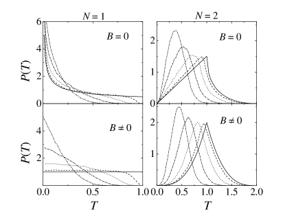
Figure 3 shows $P(T)$ for the $N=1$ and $N=2$ cases for various values of the absorption $\gamma$. One can nicely observe how the distributions for zero absorption Bar94 evolve to an exponential ($N=1$) or a convolution of exponentials ($N=2$) as the absorption strength $\gamma$ increases. For $N=1$ our simulations are in excellent agreement with the analytical expression obtained in Refs. Sch01d ; Bro97a .

Figure 3: Transmission distribution $P(T)$ for asymmetric chaotic cavities with $N=1$ and $N=2$ open channels, both cases with ($B=0$) and without $(B\neq 0$) time-reversal symmetry. We consider different absorption parameters $\gamma$: 0 (solid), 0.25 (dash), 1 (dot), 2.5 (dash dot), and 5 (dash dot dot).

Figure 4: Distributions of $dT/dE$ in units of inverse $\Delta$ for asymmetric cavities. For $N=1$ the distributions agree with Eq. (14) (dotted line), while for $N=2$ they follow Eq. (III) (dotted line).

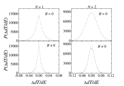
For strong absorption, $\gamma\gg 1$, we find strong numerical evidence that the distribution of individual channel-channel transmission energy derivatives, $dT_{ab}/dE$, is exponential, namely

$$\widetilde{P}_{\beta}(dT_{ab}/dE)=\frac{\lambda_{\beta}}{2}\exp\left(-\lambda_{\beta}\left|\frac{dT_{ab}}{dE}\right|\right)\,,$$ (14)

where $\lambda_{\beta}$ depends on $\gamma$, but not the channel indices $a$ and $b$. Furthermore, in this regime we find that the $dT_{ab}/dE$ for different pairs of channels are uncorrelated M-M03-2 . We conclude that either this distribution is insensitive to dynamical channel-channel correlations, or that such correlations are insignificant in our billiards. Figure 4 presents results for typical experimental values. For independent $dT_{ab}/dE$, the distribution of $dT/dE$ for $N=2$ is easily obtained by a convolution using Eq. (14) and reads

$$\widetilde{P}_{\beta}(dT/dE)=\frac{\lambda_{\beta}}{96}\exp\left(-\lambda_{\beta}\left|\frac{dT}{dE}\right|\right)$$

$$\times\left(\lambda_{\beta}^{3}\left|\frac{dT}{dE}\right|^{3}+6\lambda_{\beta}^{2}\left|\frac{dT}{dE}\right|^{2}+15\lambda_{\beta}\left|\frac{dT}{dE}\right|+15\right).\qquad$$ (15)

It remains to relate $\lambda_{\beta}$ to $\gamma$. This is done by computing $\langle(dT_{ab}/dE)^{2}\rangle$. The latter can be analytically calculated using the energy derivative of the $S$-matrix, Eq. (12), and reads M-M03-2

$$\left\langle\left(\frac{dT_{ab}}{dE}\right)^{2}\right\rangle = \frac{\pi^{2}}{\Delta^{2}}\frac{8}{\alpha^{2}(\alpha+1)^{2}}$$ (16)

$$\times \frac{\alpha^{2}+\alpha-2+4(2-\beta)}{\alpha^{2}+\alpha-2-4(2-\beta)}\,,$$

where $\alpha=N_{1}+N_{2}+\gamma$. Recalling that $\langle(dT_{ab}/dE)^{2}\rangle=2/\lambda_{\beta}^{2}$ we find $\lambda_{\beta}$ as a function of $\gamma$.

In Fig. 4 we compare the approximation $\widetilde{P}_{\beta}(dT/dE)$, where $\lambda_{\beta}$ calculated as described above, with a direct numerical simulation. The agreement is rather good.

Symmetric cavities

The influence of absorption on the transmission fluctuations is even more pronounced in billiards with reflection symmetry. In the absence of absorption the transmission distributions for reflection symmetric cavities was already analytically computed. The most salient features are the following: When time-reversal symmetry is preserved, the theory predicts that the transmission distribution $P(T)$ for reflection-symmetric cavities remains invariant when $T$ is substituted by $1-T$ GMM . On the other hand, for broken time-reversal symmetry, $P(T)$ coincides with the one for the asymmetric case, but with $T$ replaced by $1-T$ Bar96a .

To fulfill the reflection symmetry, it is sufficient to consider the $S$-matrix with the block structure GMM

$$S=\left[\begin{array}[]{cc}\frac{1}{2}(S_{1}+S_{2})&\frac{1}{2}(S_{1}-S_{2})\\ &\\ \frac{1}{2}(S_{1}-S_{2})&\frac{1}{2}(S_{1}+S_{2})\end{array}\right]\,,$$ (17)

where $S_{1}$ and $S_{2}$ are unitary (and symmetric for $\beta=1$) $N_{T}/2\times N_{T}/2$ matrices with $N_{T}=2N+N_{\phi}$. Both $S_{1}$ and $S_{2}$ have the structure given by Eq. (9).

The transmission coefficient now reads

$$T=\frac{1}{4}\sum_{a,b=1}^{N}\big{|}[{S_{1}}]_{ab}-[{S_{2}}]_{ab}\big{|}^{2}\equiv\sum_{a,b=1}^{N}\sigma_{ab}\,.$$ (18)

We numerically generate $P_{\beta}(T)$ and $\widetilde{P}_{\beta}(dT/dE)$ using the Hamiltonian approach to the $S$-matrix, Eqs. (11) and (12). Now two statistically independent matrices, $S_{1}$ and $S_{2}$, are required. We chose the dimension of $H$ to be $M=50$. For each value of $\gamma$ we obtain very good statistics with $10^{5}$ realizations.

Figure 5: Symmetric cavity transmission distributions $P(T)$ for the one- and two-channel case. For $B=0$ we consider $\gamma=0,0.5,2,2.5,$ and 10, corresponding to the solid, dashed, dotted, dashed-dotted, and dashed-dotted-dotted lines respectively. The same for the case of broken time-reversal symmetry, $B\neq 0$, but with $\gamma=0,0.25,1,2.5,$ and 5.

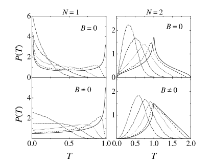
Figure 5 contrasts $P_{\beta}(T)$ obtained analytically for zero absorption Bar96a with our numerical simulations for different values of $\gamma$. Our analysis is restricted to the $N=1$ and $N=2$, as before. We observe that with increasing $\gamma$ the fingerprints of the reflection symmetry fade away, and the distributions become quite similar to those of asymmetric cavities.

As in the asymmetric case, for the strong absorption regime, $\gamma\gg 1$, our numerical simulations strongly suggest that the distribution of the energy derivative of individual channel-channel transmission coefficients $\widetilde{P}_{\beta}(dT_{ab}/dE)$ is exponential. However, in distinction to the asymmetric case, here the exponential law depends on the channels: The reflection symmetry (see Fig. 1) makes the channels (1,4) and (2,3) indistinguishable. Accordingly, we find that the “diagonal” coefficients $T_{14}$ and $T_{23}$, denoted by $\sigma_{ab}^{\rm d}$, and the “off-diagonal” ones $T_{24}$ and $T_{13}$, denoted by $\sigma_{ab}^{\rm o}$ have different variance. The second moment of the diagonal $d\sigma_{ab}^{\rm d}/dE$ is M-M03-2

$$\left\langle\left(\frac{d\sigma^{\rm d}_{ab}}{dE}\right)^{2}\right\rangle=\frac{\pi^{2}}{\Delta^{2}}\frac{4}{(\alpha^{\prime}-2){\alpha^{\prime}}^{2}(\alpha^{\prime}+1)^{2}}$$

$$\times\left[\frac{\alpha^{\prime}(\alpha^{\prime}-1)(7\beta-6)}{\alpha^{\prime}+3}+\frac{{(\alpha^{\prime}}^{2}+\alpha^{\prime}+2)(2-\beta)}{\alpha^{\prime}+1}\right]\qquad$$ (19)

whereas the off-diagonal is

$$\left\langle\left(\frac{d\sigma_{ab}^{\rm o}}{dE}\right)^{2}\right\rangle = \frac{\pi^{2}}{\Delta^{2}}\frac{2({\alpha^{\prime}}^{2}+\alpha^{\prime}+2)}{(\alpha^{\prime}-2){\alpha^{\prime}}^{2}(\alpha^{\prime}+1)^{2}(\alpha^{\prime}+3)}$$ (20)

$$\times \left[(2-\beta)\frac{\alpha^{\prime}+2}{\alpha^{\prime}+1}+4(\beta-1)\right].\qquad$$

Here, $\alpha^{\prime}=\beta(N+\gamma/2)$.

For $\gamma\gg 1$, based on the numerical simulations, we assume that $\widetilde{P}_{\beta}(d\sigma_{ab}/dE)$ is exponential and that for different pair of channels $a$ and $b$ the $d\sigma_{ab}/dE$ are uncorrelated. We then equate $\mu_{\beta}^{2}=2/\langle(d\sigma_{ab}^{\rm d}/dE)^{2}\rangle$ and $\nu_{\beta}^{2}=2/\langle(d\sigma_{ab}^{\rm o}/dE)^{2}\rangle$ to write

$$\widetilde{P}_{\beta}(dT/dE) = \frac{\mu_{\beta}^{2}\nu_{\beta}}{16}\left[\left(\frac{1}{\alpha_{1}}+\frac{1}{\alpha_{2}}\right)^{2}\exp\left(-\frac{\nu_{\beta}}{2}\left|\frac{dT}{dE}\right|\right)\right.$$ (21)

$$+ \left(\frac{1}{\alpha_{1}}-\frac{1}{\alpha_{2}}\right)\left(\frac{1}{\alpha_{1}}+\frac{1}{\alpha_{2}}+\frac{1}{\mu_{\beta}}+\left|\frac{dT}{dE}\right|\right)$$

$$\times\left.\exp\left(-\mu_{\beta}\left|\frac{dT}{dE}\right|\right)\right],$$

where $\alpha_{1}=\mu_{\beta}+\nu_{\beta}/2$, $\alpha_{2}=\mu_{\beta}-\nu_{\beta}/2$. Figure 6 compares the approximation $\widetilde{P}_{\beta}(dT/dE)$ with our numerical simulations. We chose parameters realistic to out experiment. The agreement is quite good. Deviations between the approximation (21) and the numerical simulations are of order $1/\gamma$.

Figure 6: Transmission energy derivative distributions for the symmetric chaotic cavities. The points represent the results of the simulations for $\gamma=18$ (22) for $B=0$ ($B\neq 0$) for $N=1$; $\gamma=14$ (18) for $B=0$ ($B\neq 0$) for $N=2$. The dotted lines give the approximations (14) and (21). For $N=1$ we present the diagonal case.

IV Statistical analysis of the experimental results

The statistical analysis of our experiment is based on two central hypothesis. First, as standard, we assume that the transmission fluctuations of a chaotic system are the same as those predicted by the random matrix theory Lew91 . Second, we employ an ergodic hypothesis to justify that ensemble averages are equivalent to running averages, that is, averages over the energy (frequency) and/or shape parameters. This requires RMT to be ergodic Pandey79 , which was recently shown Pluhar00 . With few exceptions (see, for instance, Ref. Hemmady04 ) this point is unnoticed.

The experimental transmission coefficients were obtained by superimposing 100 different spectra measured for billiard lengths $b$ (see Fig. 1). In the studied frequency regime there is only a single propagating mode in each of the waveguides. Hence, to every waveguide we associate a single scattering channel. For the $N=1$ case all measurements for the different combinations of entrance and exit waveguides were superimposed. The transmission for the $N=2$ case was obtained by combining the results from all $N=1$ measurements, namely, $T=T_{13}+T_{14}+T_{23}+T_{24}$.

Figure 7: Mean Transmission $\langle T\rangle$ for the $N=2$ case for $B=0$ (solid line) and $B=0.470$ T (dotted line). The Larmor resonance frequency is $\omega_{R}=2\pi\times 14.86\,$GHz)

Figure 7 shows the mean transmission ($N=2$ case) with and without applied external magnetic field. When related to experimental quantities, $\langle\cdots\rangle$ indicate running averages. Using the Weyl formula, we associate the frequency $\nu$ (actually, $\nu/\Delta$) with the energy $E$ introduced in the preceding section. The strong absorption due to the Larmor resonance is clearly seen. In App. A we discuss why is the phase-breaking effect expected to be best observed in the tails of the Larmor resonance. Figure 8 illustrates this very nicely. It shows the scaled transmission distribution $P(T/\langle T\rangle)$ for the asymmetric billiard in three different frequency windows both with and without applied external magnetic field. It is only in the frequency interval form 13.55 to 13.85 GHz that $P(T/\langle T\rangle)$ changes with magnetic field. We stress that this is different from just an absorption effect: In the frequency window around $14.45$ GHz, where the absorption is strongest, the normalized distributions with and without magnetic field are basically the same (the only difference is in the mean transmission). We identify the change in $P(T/\langle T\rangle)$ with the expected phase-breaking effect and assume that the applied magnetic field is sufficient for the ferrite cylinders to fully break time-reversal symmetry. Similar observations were made for the symmetric billiard.

Figure 8: Transmission distribution for the $N=1$ (left) and $N=2$ (right) channel cases for three different frequency windows of width $\delta\nu=0.3$ GHz centered at $\nu_{0}$ (indicated in the figure). The histograms correspond to $B=0$ (solid line) and $B=0.470$ T (dotted line).

Before we present our statistical analysis, it remains to discuss how ideal the cavity-waveguides coupling is. To determine the antenna coupling we measured the transmission through two waveguides facing each other directly. In the whole applied frequency range the total transmission was unit, with an experimental uncertainty below $5\%$, showing that the antenna coupling is perfect. There are, however reflections of about $10\%$ in amplitude from the open ends of the waveguides, where they are attached to the billiard. Small deviations from ideal coupling are also consistent, for the frequencies we work, with Ref. Men03 . Since the absorption is strong in the present experiment, and an imperfect coupling can be compensated for to a large extent by a rescaled absorption constant, we decide not to explicitly account for coupling corrections. In summary, throughout the forthcoming analysis we assume perfect coupling between the cavity and the waveguides.

For the sake of clarity, we present the statistical analysis of the asymmetric and the symmetric cavities separately.

Asymmetric cavity distributions

Figure 9 compares the experimental transmission distributions in the “phase-breaking” frequency window with the statistical theory. The absorption parameter $\gamma$, see Sec. III, was adjusted to give the best fit of the theoretical $\langle T\rangle$ to the experiment. The agreement is excellent, except for $N=2$ with $B\neq 0$.

Figure 9: Transmission distributions for the asymmetric cavity. The histograms correspond to data taken within the indicated frequency window. The dotted lines stand for the random matrix simulations, with $\gamma$ as a fitting parameter.

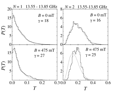
We work with a single asymmetric cavity, but use different $\gamma$ values for $N=1$ and $N=2$. The reason is simple: For $N=2$ we consider the contributions from all antennas to the transmission, whereas for $N=1$ two antennas act as additional absorption channels. This gives rise to a simple relation, namely, $\gamma^{(N=1)}=\gamma^{(N=2)}+2$.

Figure 10: Distribution of the energy derivative of the transmission for the asymmetric cavity. The dotted lines correspond to the theoretical distributions.

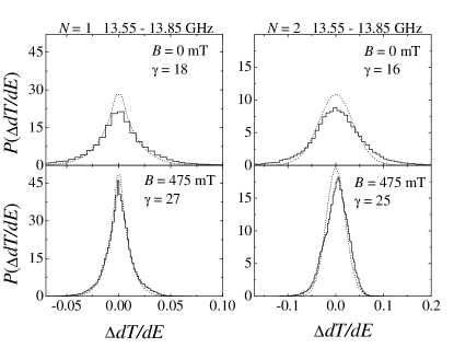
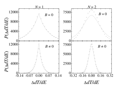
In order to compare the experimental transmission energy derivative distributions with the universal random matrix results we have to rescale the experimental data by the mean resonance spacing, namely, $dT/dE\rightarrow\Delta dT/dE$. We use the Weyl formula to estimate $\Delta$. Figure 10 shows a comparison between theoretical and experimental results for $P(\Delta dT/dE)$. Note that we take the same $\gamma$ as for $P(T)$. The signatures of the channel number, and the influence of time-reversal symmetry breaking are clearly seen. We checked that the increase in absorption when switching on the magnetic field, without switching to the unitary ensemble as well, is not sufficient to reproduce the data. Inaccuracies in the assessment of $\Delta$ provide a possible explanation for the slight disagreement between theory and experiment. The Weyl formula does not account for the standing waves in the ferrite cylinders and, thus, overestimates $\Delta$. This is consistent with Fig. 10.

Figure 11: Normalized joint distribution $F(T,dT/dE)=P(T,dT/dE)/[P(T)P(dT/dE)]$ for the asymmetric cavity for $N=1$, $B=0$. Similar result holds to $B\neq 0$.

Figure 12: Same as in Fig. 11, but with $dE/dT$ replaced by $(dT/dE)_{resc}=(dT/dE)/\sqrt{T(1-T)}$.

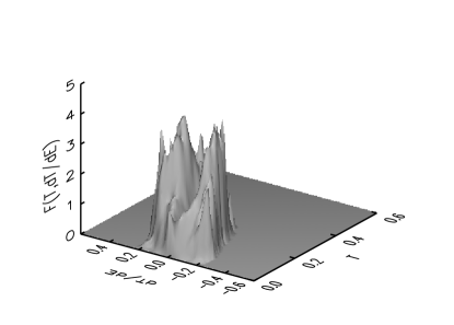
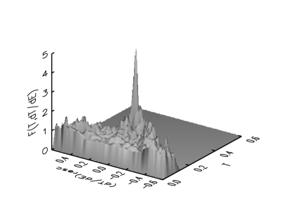
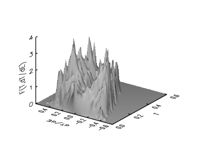
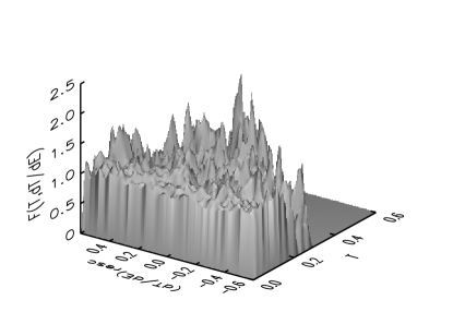
The joint distribution of $T$ and $dT/dE$ was studied in Ref. Bro97c for $N=1$ and $\gamma=0$. Remarkably, it was found that albeit $T$ and $dT/dE$ are correlated, the rescaled quantity $(dT/dE)_{\rm resc}=(dT/dE)/\sqrt{T(1-T)}$ and $T$ are not. We checked if this finding holds in our experiment, despite of absorption. Figure 11 shows the ”normalized” joint probability $F(T,\Delta dT/dE)\equiv P(T,\Delta dT/dE)/[P(T)P(\Delta dT/dE)]$ in a three dimensional representation for $N=1$ and $B=0$. A clear correlation is observed. To contrast, Fig. 12 shows $F[T,\Delta(dT/dE)_{\rm resc}]$. Here the distribution becomes flat. Unfortunately we do not have enough statistics to make a reliable determination of the distribution. A similar result, not shown here, holds for the $B\neq 0$ case.

Symmetric cavity distributions

We switch now to the statistical analysis of the symmetric cavity transmission fluctuations.

Figure 13: Transmission distributions $P(T)$ for the symmetric billiard. Histograms stand for the data taken at the indicated frequency interval, whereas the dotted lines correspond to the simulations. The absorption $\gamma$ is a fitting parameter.

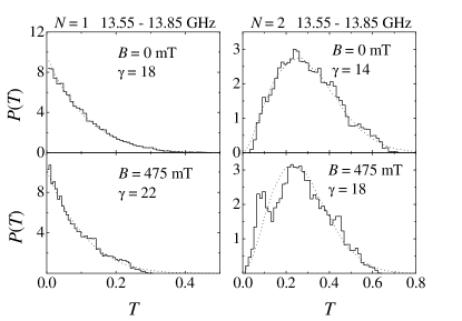
Figure 13 shows the experimental shows $P(T)$ for transmissions within $13.55\leq\nu\leq 13.85$ GHz, where the phase-breaking effect is expected to be strongest. As before, the absorption parameter $\gamma$ is the best fit of the theory to the experiment. Here, for all studied cases a nearly perfect agreement is found. Now $\gamma^{(N=1)}=\gamma^{(N=2)}+4$. This is due the reflection symmetry.

Figure 14: Distribution of the energy derivative of the transmission for the symmetric cavity. The dotted lines corresponds to the theoretical distributions obtained from random matrix theory.

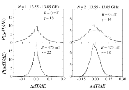
Figure 14 shows the experimental distributions $P(\Delta dT/dE)$ for the symmetric case. The signatures of the channel number and the influence of breaking time-reversal symmetry, are clearly seen. For all cases of the symmetric billiard the theoretical curves are plotted as well. We observe that the experimental distributions verify the overall trends of the theoretical predictions. In particular, the characteristic cusp at $E=0$ is nicely reproduced for $N=1$. Similar to the asymmetric case, the agreement between experiment and theory is not as good as for the transmission distribution.

Figure 15: Normalized joint distribution $F(T,dT/dE)=P(T,dT/dE)/[P(T)P(dT/dE)]$ for the symmetric cavity for $N=1$, $B=0$. Similar result holds to $B\neq 0$.

Figure 16: Same as in Fig. 15, but with $dE/dT$ replaced by $(dT/dE)_{resc}=(dT/dE)/\sqrt{T(1-T)}$.

As in the case of asymmetric cavities, theoretical calculations M-M03 show that although $T$ and $dT/dE$ are correlated, the rescaled quantity $(dT/dE)_{\rm resc}=(dT/dE)/\sqrt{T(1-T)}$ is independent of $T$. Here also the analytical results were obtained for the $N=1$ case. Fig. 15 shows the normalized joint probability $F(T,dT/dE)=P(T,dT/dE)/[P(T)P(dT/dE)]$ in a three dimensional representation for $N=1$, $B=0$ case. A clear correlation is manifest. For comparison, Fig. 16 shows the corresponding quantity for $f[T,(dT/dE)_{\rm resc}]$. Now the correlation has vanished, in accordance with theory. Similar result, not shown here, holds for the $B\neq 0$ case.

V Conclusions

This work shows that microwaves are ideally suited to experimentally verify the theory of universal transmission fluctuations through chaotic cavities. The results presented in the present paper would have been hardly accessible by any other method.

We observe a nice overall agreement between our experimental data and the random matrix results. However, the comparison between theory and microwave experiment is limited by the following issues.

In experiments, the coupling between waveguides and the cavity is usually not ideal, whereas in most theoretical works ideal coupling is assumed. In the frequency range we work Men03 supports our working hypothesis of nearly perfect coupling. In general, however, it turns out that without measuring the S matrix (with phases) it is hard to disentangle direct reflection at the cavity entrance (imperfect coupling) from absorption. From the experimental side, it would be desirable to have a better handle on absorption.

Microwave systems are usually time-reversal invariant, and as we have seen it is not trivial to break this symmetry. At the same time we increase the magnetic field, turning on the phase-breaking mechanism, absorption also increases. Unfortunately, both effects are inextricable. This is why it is beyond our present experimental capability to quantitatively investigate the transmission fluctuations along the crossover regime between preserved and broken time-reversal invariance. Actually, to compare theory with experimental results we assume that the transmission data at $B=0.470$ mT and $13.55<\nu<13.85$ GHz are far beyond the crossover regime.

We hope that the present work will trigger additional theoretical effort in the mentioned directions.

Appendix A Phase-breaking properties of the ferrite

This appendix is devoted to the discussion of the ferromagnetic resonance and the phase-breaking mechanism. For that purpose we first quickly present some elements of the well-established theory of microwave ferrites, see for instance, Ref. lax62, .

For the sake of simplicity, we first restrict ourselves to the situation of an incoming plane wave reflected by the surface of an semi-infinite ferrite medium. We assume that incoming, reflected, and refracted waves propagate in the $xy$ plane and are polarized along the $z$ direction, and that there is an externally applied static magnetic field in the $z$ direction, as shown in Fig. 17. We ask what is the phase acquired due to the reflection on the ferrite.

To answer this question we need to solve Maxwell’s equations. For this geometry and single-frequency electromagnetic fields, like our microwaves, this is a simple task. The ferrite properties come into play by the constitutive relations ${\bf D}=\epsilon_{0}\epsilon{\bf E}$ and ${\bf B}=\mu_{0}\mu{\bf H}$, more specifically through the permeability $\mu$, that is a tensor with the form

$$\mu=1+\chi=\left(\begin{array}[]{ccc}1+\chi_{r}&-\imath\chi_{i}&\cdot\\ \imath\chi_{i}&1+\chi_{r}&\cdot\\ \cdot&\cdot&1+\chi_{0}\end{array}\right)\,.$$ (22)

with

$$\chi_{r}=\frac{\omega_{L}\omega_{M}}{\omega_{L}^{2}-\hat{\omega}^{2}}\,,\quad\chi_{i}=-\frac{\hat{\omega}\omega_{M}}{\omega_{L}^{2}-\hat{\omega}^{2}}\,,\quad\hat{\omega}=\omega+\imath\lambda\,.$$ (23)

Here $\omega_{L}=-\gamma H_{0}$ and $\omega_{M}=\gamma M_{0}$ are the precession angular frequencies about the external field $H_{0}$ and the equilibrium magnetization $M_{0}$, respectively. $\mu_{0}$ is the static susceptibility. More details can be found, for instance, in Chapter 2.2.3 of Ref. Stoe99 .

Figure 17: Plane wave reflected by the surface of a ferrite slab.

We solve the proposed problem using for the electric field the ansatz ${\bf E}(r)=E(r){\bf e_{z}}$, where

$$E(r)=\left\{\begin{array}[]{lc}E_{T}e^{\imath{\bf k}_{T}\cdot{\bf r}}\,,&x<0\,,\\ E_{I}e^{\imath{\bf k}_{I}\cdot{\bf r}}+E_{R}e^{\imath{\bf k}_{R}\cdot{\bf r}}\,,&x>0\,,\end{array}\right.$$ (24)

with ${\bf k}_{I}=k_{0}(-\cos\alpha,\sin\alpha\,,0)\,$, ${\bf k}_{R}=k_{0}(\cos\alpha,\sin\alpha\,,0)\,$, ${\bf k}_{T}=k(-\cos\beta,\sin\beta\,,0)$, see Fig. 17.

The derivation of the amplitudes $E_{I}$,$E_{R}$ and $E_{T}$ is similar to that of Fresnel’s formula (see, for instance, Jac62 ). Since an explicit calculation for ferrites is given in Vra02 , only the results shall be given. Using the continuity of ${\bf E}_{\parallel}$, ${\bf D}_{\perp}$, ${\bf B}_{\perp}$ and ${\bf H}_{\parallel}$ on the boundary, one writes

$$E_{T}=E_{I}+E_{R}\qquad\mbox{and}\qquad k\sin\beta=k_{0}\sin\alpha$$ (25)

which is just Snell’s law. For the relative amplitude of the reflected part we obtain

$$\frac{E_{R}}{E_{I}}=\frac{(n^{2}/\epsilon)\cos\alpha+\imath\delta\sin\alpha-\sqrt{n^{2}-\sin^{2}\alpha}}{(n^{2}/\epsilon)\cos\alpha-\imath\delta\sin\alpha+\sqrt{n^{2}-\sin^{2}\alpha}}$$ (26)

where

$$n^{2}=\frac{(\omega_{L}+\omega_{M})^{2}-\hat{\omega}^{2}}{\omega_{L}(\omega_{L}+\omega_{M})-\hat{\omega}^{2}}$$ (27)

and

$$\delta=\frac{\chi_{i}}{1+\chi_{r}}=-\frac{\hat{\omega}\omega_{M}}{\displaystyle\omega_{L}(\omega_{L}+\omega_{M})-\hat{\omega}^{2}}\,.$$ (28)

Note that there is a term depending on the sign of $\alpha$, i.e. on the direction of the incident wave. This term is responsible for the phase-breaking effect.

The above formulas have to be modified when dealing with a ferrite of finite width. For a slab of thickness $l$ and $\alpha=0$ we have

$$\frac{E_{T}}{E_{I}}=\frac{4\frac{\epsilon}{n}}{(1+\frac{\epsilon}{n})^{2}e^{\imath k(1-n)l}-(1-\frac{\epsilon}{n})^{2}e^{\imath k(1+n)l}}$$ (29)

and

$$\frac{E_{R}}{E_{I}}=-2\imath\sin{knl}\frac{1-\frac{\epsilon^{2}}{n^{2}}}{(1+\frac{\epsilon}{n})^{2}e^{\imath k(1-n)l}-(1-\frac{\epsilon}{n})^{2}e^{\imath k(1+n)l}}\,.$$ (30)

In contrast to Eq. (26), $E_{T}$ is no longer the amplitude of the transmitted wave propagating inside the ferrite. Here $E_{T}$ is the amplitude of the wave that crossed the ferrite slab an emerged at the other side. The explicit formula for $\alpha\neq 0$ is lengthy and is not be presented here.

The phase-breaking becomes clearly manifest by writing Eq. (30) as

$$\frac{E_{R}}{E_{I}}=\left|\frac{E_{R}}{E_{I}}\right|e^{i\phi_{\rm refl}(\alpha).}$$ (31)

where $\phi_{\rm refl}(\alpha)$ is the phase acquired due to reflection. Figure 18 shows modulus of transmission $|E_{T}/E_{I}|$ and reflection $|E_{R}/E_{I}|$ as well as the phase shift for different incidence angles and $l=1\,$mm, the thickness of our ferrite cylinders. The curves are calculated using the ferrite parameters (see caption of Fig. 18) given by the supplier. We find a resonance angular frequency of $\omega_{R}=\sqrt{\omega_{L}(\omega_{L}+\omega_{M})}=2\pi\times 14.86\,$GHz. This resonance corresponds to the dominant structure observed in Fig. 18. The additional substructures are due to standing waves inside the ferrite.

Figure 18: Reflection, transmission, and phase shift for a ferrite slab ($M_{0}=$130 mT, $\epsilon=$15, $\lambda=0.1\,$GHz) of thickness $l=$1 mm at $B_{0}=\mu_{0}H_{0}=$470 mT for different incidence angles $\alpha$.

Figure 19: Difference $\Delta\phi=\phi_{\rm refl}(\alpha)-\phi_{\rm refl}(-\alpha)$ of phase shifts observed between an incoming wave and its time-reversed equivalent.

To illustrate the phase-breaking effect of the ferrite, in Fig. 19 we show the phase difference $\Delta\phi=\phi_{\rm refl}(\alpha)-\phi_{\rm refl}(-\alpha)$ between the incoming and the time-reversed wave. We see that the effect is maximal at the resonance frequency, and vanishes as one moves off-resonance. Unfortunately, the absorption is maximal at the resonance too. This are the quantitative observations in support of the discussion presented in Sec. II.

Figure 20: Experimental reflection for a ferrite slab of thickness $l=$1mm (a) and 2 mm (b). The dashed lines have been calculated by superimposing the results for two different internal magnetizations $M_{0}=$110 mT an 190 mT. The broad minimum observed for $l=$2 mm close to 13 GHz is due to a standing wave within the ferrite. For $l=$1 mm the corresponding minimum is at 15 GHz and superimposes the ferromagnetic resonance.

Finally, to experimentally check the properties of the ferrites, we place a small sheet of the material between two waveguide facing each other. Two different thicknesses $l=1\,$mm and $2\,$mm were used. Figure 20 shows the measured reflection $|E_{R}/E_{I}|$ as a function of $\nu$. The small oscillations superimposing the dominant resonance structures correspond to standing waves within the waveguide and are an artifact of the experiment. Comparing the experimental results with the calculation shown in Fig. 18, we notice that the assumption of a single homogenous internal magnetization is not in accordance with the measurement. The dashed line is obtained by superimposing the theoretical results for two different values of the magnetization. The overall behavior of the resonance structures becomes then in qualitatively agreement with the data.

References

- (1) C. W. J. Beenakker, Rev. Mod. Phys. 69, 731 (1997).
- (2) C. M. Marcus, A. J. Rimberg, R. M. Westervelt, P. F. Hopkins, and A. C. Gossard, Phys. Rev. Lett. 69, 506 (1992).
- (3) H. U. Baranger and P. A. Mello, Phys. Rev. Lett. 73, 142 (1994).
- (4) R. A. Jalabert, J.-L. Pichard, and C. W. J. Beenakker, Europhys. Lett. 27, 255 (1994).
- (5) A. G. Huibers, M. Switkes, C. M. Marcus, K. Campman, and A. C. Gossard, Phys. Rev. Lett. 81, 200 (1998).
- (6) H. U. Baranger and P. A. Mello, Phys. Rev. B 51, 4703 (1995).
- (7) A. G. Huibers, S. R. Patel, C. M. Marcus, P. W. Brouwer, C. I. Duruöz, and J. S. Harris, Jr., Phys. Rev. Lett. 81, 1917 (1998).
- (8) E. Doron, U. Smilansky, and A. Frenkel, Phys. Rev. Lett. 65, 3072 (1990).
- (9) R. A. Jalabert, H. U. Baranger, and A. D. Stone, Phys. Rev. Lett. 65, 2442 (1990).
- (10) H. Schanze, E. R. P. Alves, C. H. Lewenkopf, and H.-J. Stöckmann, Phys. Rev. E 64, 065201(R) (2001).
- (11) Y.-H. Kim, M. Barth, H.-J. Stöckmann, and J. Bird, Phys. Rev. B 65, 165317 (2002).
- (12) P. So, S. Anlage, E. Ott, and R. Oerter, Phys. Rev. Lett. 74, 2662 (1995).
- (13) U. Stoffregen, J. Stein, H.-J. Stöckmann, M. Kuś, and F. Haake, Phys. Rev. Lett. 74, 2666 (1995).
- (14) E. Kogan, P. A. Mello, and H. Liqun, Phys. Rev. E 61, R17 (2000).
- (15) C. W. J. Beenakker and P. W. Brouwer, Physica E 9, 463 (2001).
- (16) P. W. Brouwer, Phys. Rev. B 51, 16878 (1995).
- (17) M. Martínez and P. A. Mello, Phys. Rev. E 63, 016205 (2000).
- (18) H. U. Baranger and P. A. Mello, Phys. Rev. B 54, 14297 (1996).
- (19) P. W. Brouwer, S. A. van Langen, K. M. Frahm, M. Büttiker, and C. W. J. Beenakker, Phys. Rev. Lett. 79, 913 (1997).
- (20) S. A. van Langen, P. Silvestrov, and C. W. J. Beenakker, Stud. Appl. Math. 23, 691 (1998).
- (21) M. Martínez-Mares, unpublished.
- (22) M. Vraničar, M. Barth, G. Veble, M. Robnik, and H.-J. Stöckmann, J. Phys. A 35, 4929 (2002).
- (23) P. A. Mello and H. U. Baranger, Waves Random Media 9, 105 (1999).
- (24) T. Guhr, A. Müller-Groeling, and H. A. Weidenmüller, Phys. Rep. 299, 189 (1998).
- (25) C. H. Lewenkopf and H. A. Weidenmüller, Ann. Phys. (N.Y.) 212, 53 (1991).
- (26) É. R. P. Alves and C. H. Lewenkopf, Phys. Rev. Lett. 88, 256805 (2002); C. H. Lewenkopf, Chaos, Solitons and Fractals 16, 449 (2003).
- (27) C. H. Lewenkopf, A. Müller, and E. Doron, Phys. Rev. A 45, 2635 (1992).
- (28) P. W. Brouwer and C. W. J. Beenakker, Phys. Rev. B 55, 4695 (1997).
- (29) J. J. M. Verbaarschot, H. A. Weidenmüller, and M. R. Zirnbauer, Phys. Rep. 129, 367 (1985).
- (30) P. W. Brouwer, K. M. Frahm, and C. W. J. Beenakker, Phys. Rev. Lett. 78, 4737 (1997).
- (31) M. Martínez-Mares, unpublished.
- (32) V. A. Gopar, M. Martínez, P. A. Mello, and H. U. Baranger, J. Phys. A 29, 881 (1996).
- (33) B. Lax and K. Button, Microwave Ferrites and Ferrimagnetics (McGraw-Hill, New York, 1962).
- (34) H.-J. Stöckmann, Quantum Chaos - An Introduction (Cambridge University Press, Cambridge, 1999).
- (35) J. D. Jackson, Classical Electrodynamics (Wiley, New York, 1962).
- (36) R. A. Méndez-Sánchez, U. Kuhl, M. Barth, C. H. Lewenkopf, and H. J. Stoeckmann, Phys. Rev. Lett. 91, 174102 (2003).
- (37) S. Hemmady, X. Zheng, E. Ott, T. M. Antonsen, and S. M. Anlage, cond-mat/0403225.
- (38) A. Pandey, Ann. Phys. (N.Y.) 119, 170 (1979).
- (39) Z. Pluhař and H. A. Weidenmüller, Phys. Rev. Lett. 84, 2833 (2000).