Molecular dynamics and theory for the contact values of the radial distribution functions of hard-disk fluid mixtures

Abstract

We report molecular dynamics results for the contact values of the radial distribution functions of binary additive mixtures of hard disks. The simulation data are compared with theoretical predictions from expressions proposed by Jenkins and Mancini [J. Appl. Mech. 54, 27 (1987)] and Santos et al. [J. Chem. Phys. 117, 5785 (2002)]. Both theories agree quantitatively within a very small margin, which renders the former still a very useful and simple tool to work with. The latter (higher-order and self-consistent) theory provides a small qualitative correction for low densities and is superior especially in the high-density domain.

I Introduction

Model systems of hard disks and hard spheres are useful for the derivation of rigorous results in statistical mechanics as well as in perturbation theories of fluids.HM86 Hard disks and hard spheres are also relevant for the modeling of mesoscopic systems such as colloidal suspensionsL94 and granular matter.C90 Apart from its academic interest, the study of two-dimensional systems is important in the context of monolayer adsorption on solid surfaces.S76 Recently, the equation of state of hard disks has been experimentally measured in charge-stabilized colloidal particles suspended in water and confined by a laser beam.BBHG03 While most of the studies are restricted to monodisperse fluids, it is obviously important to consider the polydisperse character of the system, especially in applications to mesoscopic matter. The equation of state, as well as nonequilibrium transport properties, of bidisperse systems of inelastic hard disks have been discussed in the literature, see Refs. JM87, ; willits99, ; alam02, ; alam02b, ; alam03, ; garzo03, ; garzo03b, ; MG03, ; rahaman03, ; dahl03, ; dahl04, and references therein.

The state of an additive $m$-component fluid mixture of $N=\sum_{i=1}^{m}N_{i}$ hard disks is characterized by the total number density $\rho$, the set of mole fractions $\textbf{x}\equiv\{x_{1},x_{2},\ldots,x_{m}\}$, with $x_{i}=N_{i}/N$, and the set of diameters $\bm{\sigma}\equiv\{\sigma_{1},\sigma_{2},\ldots,\sigma_{m}\}$. Instead of $\rho$, the area fraction $\nu=(\pi/4)\rho\langle\sigma^{2}\rangle$, where $\langle\sigma^{n}\rangle\equiv\sum_{i}x_{i}\sigma_{i}^{n}$ is the $n$-th moment of the size distribution, can be used to characterize the density of the system. The spatial correlation between two disks of species $i$ and $j$ separated by a distance $r$ is measured by the radial distribution function (RDF) $g_{ij}(r;\nu,\textbf{x},\bm{\sigma})$. The contact values

$$\chi_{ij}(\nu,\textbf{x},\bm{\sigma})\equiv g_{ij}(\sigma_{ij};\nu,\textbf{x},\bm{\sigma}),\quad\sigma_{ij}\equiv(\sigma_{i}+\sigma_{j})/2,$$ (1)

of the RDFs are of special interest since they appear in the Enskog kinetic theory of dense fluidsFK72 and, more important, they are directly related to the equation of state (EOS) of the fluid via the virial theorem,RS82

$$Z(\nu,\textbf{x},\bm{\sigma}) \equiv \frac{p}{\rho k_{B}T}$$ (2)

$$= 1+2\nu\sum_{i,j}x_{i}x_{j}\frac{\sigma_{ij}^{2}}{\langle\sigma^{2}\rangle}\chi_{ij}(\nu,\textbf{x},\bm{\sigma}).$$

Alternatively, the compressibility factor $Z$ can be expressed asNHSC98

$$Z_{w}(\nu,\textbf{x},\bm{\sigma})=\sum_{i}x_{i}\chi_{iw}(\nu,\textbf{x},\bm{\sigma}),$$ (3)

where $\chi_{iw}(\nu,\textbf{x},\bm{\sigma})$ denotes the density of species $i$ at contact with a planar hard wall, relative to the associated bulk density. Its expression can be obtained from that of $\chi_{ij}(\nu,\textbf{x},\bm{\sigma})$ by assuming the wall to be a component of the mixture present in zero concentration and having an infinite diameter:NHSC98 ; HAB76

$$\chi_{iw}(\nu,\textbf{x},\bm{\sigma})=\lim_{\sigma_{j}\to\infty}\,\,\lim_{x_{j}\to 0}\,\chi_{ij}(\nu,\textbf{x},\bm{\sigma}).$$ (4)

The subscript $w$ in $Z_{w}$ has been used to emphasize that Eq. (3) represents a route alternative to Eq. (2) to get the EOS of the hard-disk polydisperse fluid. Of course, $Z=Z_{w}$ in an exact description, but $Z$ and $Z_{w}$ may differ when dealing with approximations. Thus a stringent consistency condition for an approximate theory of $\chi_{ij}$ is to yield the same EOS through both routes.

The aim of this paper is two-fold. First, we present (new, accurate) molecular dynamics results for $\chi_{ij}$ in the case of a bidisperse hard-disk fluid mixture with a size ratio $\sigma_{1}/\sigma_{2}=1/2$. Next, those simulation data are compared against theoretical predictions by Jenkins and ManciniJM87 and by Santos et al.SYH02 As will be seen, both theories agree quantitatively well with the simulation data but the latter is slightly superior in the high-density fluid regime ($0.3\lesssim\nu\lesssim 0.7$). The theoretical proposals for $\chi_{ij}$ are presented in Sec. II and the simulation method is outlined in Sec. III. The results are presented and discussed in Sec. IV and we close the paper in Sec. V with some final remarks.

II Theoretical approximations

In this section, different approximations for the contact values of the radial distribution function are reviewed, first for the monodisperse and then for the polydisperse case.

II.1 The monodisperse case

For the sake of completeness, let us begin with the one-component fluid before considering the more general polydisperse fluid. Perhaps the most widely used approximation for the contact value $\chi(\nu)$ of the RDF of the monodisperse hard-disk fluid is the one proposed by Henderson in 1975:H75

$$\chi^{\text{H}}(\nu)=\frac{1-7\nu/16}{(1-\nu)^{2}}.$$ (5)

Despite the simplicity of this prescription, it provides fairly accurate values. On the other hand, Eq. (5) tends to overestimate the value of $\chi(\nu)$ for high densities of the stable fluid phase.VL82 ; SHY95 ; MCG97 This led Verlet and LevesqueVL82 to propose the correction

$$\chi^{\text{VL}}(\nu)=\chi^{\text{H}}(\nu)-\frac{\nu^{3}}{2^{6}(1-\nu)^{4}}.$$ (6)

A more accurate prescription has recently been proposed by one of us:Lu01 ; Lu01b ; Lu02 ; Lu04

$$\chi^{\text{L4}}(\nu) = \frac{1}{2}\left[\chi^{\text{H}}(\nu)+\chi^{\text{VL}}(\nu)\right]$$ (7)

$$= \chi^{\text{H}}(\nu)-\frac{\nu^{3}}{2^{7}(1-\nu)^{4}}.$$

This is confirmed by Fig. 1, where simulation data of $\chi(\nu)$,EL85 ; Lu01 ; Lu02 ; Lu04 relative to Henderson’s approximation $\chi^{\text{H}}(\nu)$, are compared with the ratios $\chi^{\text{VL}}(\nu)/\chi^{\text{H}}(\nu)$ and $\chi^{\text{L4}}(\nu)/\chi^{\text{H}}(\nu)$. We observe that $\chi^{\text{H}}(\nu)$ behaves satisfactorily up to an area fraction $\nu\approx 0.3$. However, as the density increases and approaches the limit of stability of the hard-disk fluid ($\nu\simeq 0.7$),J99 ; Lu01 ; Lu01b ; Lu04 ; Lu02 $\chi^{\text{H}}(\nu)$ overestimates the simulation data (by a few percent at $\nu=0.68$), while Eq. (7) presents an excellent agreement with computer simulations for densities $\nu\leq 0.68$.

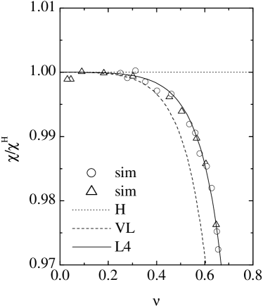
Figure 1: Density dependence of the ratio $\chi/\chi^{\text{H}}$, where unity (dotted line) corresponds to Eq. (5). The circlesLu01 ; Lu02 ; Lu04 and trianglesEL85 are simulation data, while the dashed and solid lines are the theoretical predictions given by Eqs. (6) and (7), respectively.

II.2 The polydisperse case

In this subsection, the classical result for the RDF contact valueJM87 is confronted to more recent findings.SYH02 The derivation is detailed for bulk- and wall-EOS in both cases, and the agreement/disagreement of the two approaches is discussed.

II.2.1 Jenkins and Mancini’s approximation

In the case of a hard-disk mixture, a useful approximation for the contact values $\chi_{ij}$ was proposed by Jenkins and Mancini in 1987.JM87 It reads

$$\chi_{ij}^{\text{JM}}(\nu,\textbf{x},\bm{\sigma})=\frac{1}{1-\nu}+\frac{9}{16}\frac{\nu}{(1-\nu)^{2}}z_{ij}(\textbf{x},\bm{\sigma}),$$ (8)

where the parameter

$$z_{ij}(\textbf{x},\bm{\sigma})\equiv\frac{\sigma_{i}\sigma_{j}}{\sigma_{ij}}\frac{\langle\sigma\rangle}{\langle\sigma^{2}\rangle}$$ (9)

contains the whole dependence of $\chi_{ij}$ on the size composition through the first two moments. It is worth mentioning that Eq. (8) was originally proposed in the context of inelastic disks and thus it is much better known by researchers in granular matter theory than by researchers in liquid theory. As a matter of fact, Eq. (8) has recently been rediscovered by liquid theorists.BS01

In the special case where all the disks have the same diameter ($\sigma_{i}\to\sigma$), one has $z_{ij}\to 1$ and so Eq. (8) reduces to Henderson’s approximation (5) for monodisperse disks. Thus, Jenkins and Mancini’s approximation (8) represents a simple, straightforward extension of $\chi^{\text{H}}$ to the polydisperse case. As a consequence, it inherits, by construction, the limitations of Henderson’s equation (5) for high densities (cf. Fig. 1). Moreover, Eq. (8) does not yield the same EOS through routes (2) and (3). Let us first consider the standard route (2). Taking into account the mathematical identities (for an arbitrary number of components)

$$\sum_{i,j}x_{i}x_{j}\sigma_{ij}^{2}=\frac{\langle\sigma^{2}\rangle+\langle\sigma\rangle^{2}}{2},$$ (10)

$$\sum_{i,j}x_{i}x_{j}\sigma_{ij}^{2}z_{ij} = \frac{\langle\sigma\rangle}{2\langle\sigma^{2}\rangle}\sum_{i,j}x_{i}x_{j}\sigma_{i}\sigma_{j}(\sigma_{i}+\sigma_{j})$$ (11)

$$= \langle\sigma\rangle^{2},$$

insertion of Eq. (8) into Eq. (2) yields

$$Z^{\text{JM}}(\nu,\textbf{x},\bm{\sigma}) = 1+\frac{\nu}{1-\nu}+\mathcal{A}\nu\frac{1+\nu/8}{(1-\nu)^{2}}$$ (12)

$$= 1+2\nu\left[\frac{1-{\cal A}}{2(1-\nu)}+{\cal A}\chi^{\text{H}}(\nu)\right]~{},$$

where ${\cal A}\equiv{\langle\sigma\rangle^{2}}/{\langle\sigma^{2}\rangle}$ was used as a convenient abbreviation.Lu01b ; Lu02 To explore the alternative route (3), let us take the limits indicated in Eq. (4) on Eq. (8) to get

$$\chi_{iw}^{\text{JM}}(\nu,\textbf{x},\bm{\sigma})=\frac{1}{1-\nu}+\frac{9}{16}\frac{\nu}{(1-\nu)^{2}}\,z_{iw}(\textbf{x},\bm{\sigma}),$$ (13)

where

$$z_{iw}(\textbf{x},\bm{\sigma})\equiv 2\sigma_{i}\frac{\langle\sigma\rangle}{\langle\sigma^{2}\rangle}.$$ (14)

Inserting Eq. (13) into Eq. (3) and making use of

$$\sum_{i}x_{i}z_{iw}=2\mathcal{A},$$ (15)

one has

$$Z_{w}^{\text{JM}}(\nu,\textbf{x},\bm{\sigma}) = \sum_{i}x_{i}\chi_{iw}^{\text{JM}}(\nu,\textbf{x},\bm{\sigma})$$ (16)

$$= Z^{\text{JM}}(\nu,\textbf{x},\bm{\sigma})+\mathcal{A}\frac{\nu/8}{(1-\nu)}~{}.$$

The inconsistency $Z^{\text{JM}}\neq Z_{w}^{\text{JM}}$ appears already to first order in $\nu$. Comparison with simulation results shows that $Z^{\text{JM}}$ is clearly superior to $Z_{w}^{\text{JM}}$.

II.2.2 Santos, Yuste, and López de Haro’s approximation

The two limitations of $\chi_{ij}^{\text{JM}}$ just mentioned, namely the slavery to Henderson’s equation $\chi^{\text{H}}$ and the failure to give a common EOS through Eqs. (2) and (3), are remedied by a recent proposal made by Santos et al.SYH02 It reads

$$\chi_{ij}^{\text{SYH}}(\nu,\textbf{x},\bm{\sigma}) = \frac{1}{1-\nu}$$

$$+\left[(2-\nu)\chi(\nu)-\frac{2-\nu/2}{1-\nu}\right]z_{ij}(\textbf{x},\bm{\sigma})$$

$$+\left[\frac{1-\nu/2}{1-\nu}-(1-\nu)\chi(\nu)\right]z_{ij}^{2}(\textbf{x},\bm{\sigma})~{},$$

where $z_{ij}$ is again given by Eq. (9) and the contact value $\chi(\nu)$ of the monodisperse fluid can be freely chosen. Obviously, in the trivial case where all the disks have the same size, $z_{ij}=1$ and so $\chi_{ij}^{\text{SYH}}(\nu)=\chi(\nu)$. Insertion of Eq. (II.2.2) into Eq. (2) yields the following simple form:

$$Z^{\text{SYH}}(\nu,\textbf{x},\bm{\sigma}) = 1+\frac{\nu}{1-\nu}+\mathcal{A}\nu\left[2\chi(\nu)-\frac{1}{1-\nu}\right]$$ (18)

$$= 1+2\nu\left[\frac{1-{\cal A}}{2(1-\nu)}+{\cal A}\chi(\nu)\right]~{},$$

where use has been made of Eqs. (10), (11), and

$$\sum_{i,j}x_{i}x_{j}\sigma_{ij}^{2}z_{ij}^{2} = \frac{\langle\sigma\rangle^{2}}{\langle\sigma^{2}\rangle^{2}}\sum_{i,j}x_{i}x_{j}\sigma_{i}^{2}\sigma_{j}^{2}$$ (19)

$$= \langle\sigma\rangle^{2},$$

valid again for any number of components. Note the identical form of the second lines in both Eq. (12) and Eq. (18). The expression for $\chi_{iw}^{\text{SYH}}$ is given by Eq. (II.2.2), except that $z_{ij}$ must be replaced by $z_{iw}$. When $\chi_{iw}^{\text{SYH}}$ is inserted into Eq. (3) and use is made of Eq. (15) and of

$$\sum_{i}x_{i}z_{iw}^{2}=4\mathcal{A},$$ (20)

it turns out that the EOS (18) is consistently reobtained, i.e. $Z^{\text{SYH}}_{w}\equiv Z^{\text{SYH}}$.

So far, the monodisperse quantity $\chi(\nu)$ remains arbitrary. From that point of view, Eq. (II.2.2) represents a consistent class of approximations, with free $\chi(\nu)$, rather than a specific approximation.

II.2.3 Some comments

It is worth mentioning that Eqs. (8) and (II.2.2) share the property that, at a given packing fraction $\nu$, the whole dependence of $\chi_{ij}$ on the composition $(\textbf{x},\bm{\sigma})$ of the mixture appears through the parameter $z_{ij}$ only. To clarify the implications of this, let us consider two mixtures M and M’ having the same packing fraction $\nu$ but strongly differing in the set of mole fractions, the sizes of the particles, and even the number of components, i.e. $(\textbf{x},\bm{\sigma})\neq(\textbf{x}^{\prime},\bm{\sigma}^{\prime})$. Suppose now that there exists a pair $ij$ in mixture M and another pair $i^{\prime}j^{\prime}$ in mixture M’ such that $z_{ij}(\textbf{x},\bm{\sigma})=z_{i^{\prime}j^{\prime}}(\textbf{x}^{\prime},\bm{\sigma}^{\prime})$. Then, according to Eqs. (8) and (II.2.2), the contact value of the RDF for the pair $ij$ in mixture M is the same as that for the pair $i^{\prime}j^{\prime}$ in mixture M’. This sort of “universality” ansatz, which is more general than Eqs. (8) or (II.2.2) and is shared by other well-known proposals for $\chi_{ij}$ of hard-sphere fluids (e.g. the scaled-particle-theory, Percus–Yevick, and Boublík–Grundke–Henderson–Lee–Levesque approximations),SYH02 is of course only approximate. However, its enforcement leads to the construction of simple and accurate proposals for $\chi_{ij}$ with the help of only a few requirements.SYH02 ; SYH99

Interestingly enough, the EOS (12) and (18) are identical when $\chi=\chi^{\text{H}}$ is used in the latter, even though the contact values $\chi_{ij}$ used in the derivation are different. More specifically, if $\chi=\chi^{\text{H}}$ is used in Eq. (II.2.2), then

$$\chi_{ij}^{\text{SYH}}-\chi_{ij}^{\text{JM}}=\frac{\nu/16}{1-\nu}z_{ij}\left(1-z_{ij}\right).$$ (21)

The property $Z^{\text{SYH}}=Z^{\text{JM}}$ is just a consequence of $\sum_{i,j}x_{i}x_{j}\sigma_{ij}^{2}z_{ij}=\sum_{i,j}x_{i}x_{j}\sigma_{ij}^{2}z_{ij}^{2}$, as follows from Eqs. (11) and (19).

If one chooses $\chi(\nu)=\chi^{\text{H}}(\nu)$ then Eq. (II.2.2), being consistent with the condition $Z=Z_{w}$, can be expected to become more accurate than Eq. (8), especially for highly asymmetric mixtures. Since $\chi^{\text{H}}(\nu)$ is fairly good for $\nu\lesssim 0.3$, as Fig. 1 shows, the main difference between Eqs. (8) and (II.2.2) in that density domain lies in the functional relation on the parameter $z_{ij}$: linear in the case of Eq. (8), quadratic in the case of Eq. (II.2.2). As a consequence,

$$\chi_{ij}^{\text{SYH}}/\chi_{ij}^{\text{JM}} > 1\quad\text{if }z_{ij}<1,$$ (22)

$$= 1\quad\text{if }z_{ij}=1,$$

$$< 1\quad\text{if }z_{ij}>1,$$

where we emphasize that (22) refers to $0<\nu\lesssim 0.3$. This is illustrated in Fig. 2, where the ratio $\chi_{ij}^{\text{SYH}}/\chi_{ij}^{\text{JM}}$ is plotted versus $z_{ij}$ for $\nu=0.25$ and $\nu=0.5$. In the former case, since $\chi^{\text{H}}$ and $\chi^{\text{L4}}$ yield practically the same value, the associated two functions given by Eq. (II.2.2) are hardly distinguishable. On the other hand, those functions exhibit visible small differences at $\nu=0.5$ due to the fact that $\chi^{\text{H}}$ deviates from $\chi^{\text{L4}}$ by about $0.5\%$ (cf. Fig. 1).

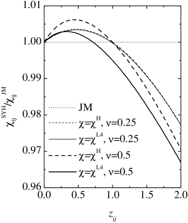
Figure 2: Plot of the ratio $\chi_{ij}^{\text{SYH}}/\chi_{ij}^{\text{JM}}$ against the parameter $z_{ij}$ for $\nu=0.25$ (thin lines) and $\nu=0.50$ (thick lines). The dashed lines correspond to the choice $\chi(\nu)=\chi^{\text{H}}(\nu)$ in Eq. (II.2.2), while the solid lines correspond to the choice $\chi(\nu)=\chi^{\text{L4}}(\nu)$. The dotted line represents the JM expression (8).

In the spirit of the approximations (II.2.2) and (18), the more accurate the monodisperse function $\chi(\nu)$ the better. Therefore, more successful predictions for $\chi_{ij}$ and $Z$ can be expected if one chooses for $\chi(\nu)$ an expression more refined than Henderson’s, such as Eq. (7), especially for high densities. In Sec. IV we will check all these expectations by comparing molecular dynamics results for $\chi_{ij}$ against Eqs. (8) and (II.2.2), the latter being complemented by the monodisperse prescriptions (5) and (7).

III Simulation method

Since we are interested in the behavior of rigid particles, we use an event-driven (ED) method that discretizes the sequence of events with variable time steps for all particles between collisions, as adapted to the problem. This is different from classical molecular dynamics simulations, where the time step is usually fixed for the numerical integration of the equations of motion.

III.1 Collision Model

The particles are assumed to be perfectly rigid and follow an undisturbed motion until a collision occurs as described below. A change in velocity can occur only at a collision, and due to their rigidity, the disks collide instantaneously. The standard interaction model for instantaneous collisions of particles with diameters $\sigma_{i}$ and mass $m_{i}$ is used in the following. The post-collisional velocities $(\mathbf{v}_{i}^{\prime},\mathbf{v}_{j}^{\prime})$ of two collision partners $ij$ are given, in terms of the pre-collisional velocities $(\mathbf{v}_{i},\mathbf{v}_{j})$, by

$$\mathbf{v}_{i,j}^{\prime}=\mathbf{v}_{i,j}\mp\frac{2~{}\mu_{ij}}{m_{i,j}}\mathbf{v}_{n}~{},$$ (23)

where $\mu_{ij}=m_{i}m_{j}/(m_{i}+m_{j})$ is the reduced mass and $\mathbf{v}_{n}\equiv\left[(\mathbf{v}_{i}-\mathbf{v}_{j})\cdot{\mathbf{n}}\right]{\mathbf{n}}$ is the component of the relative velocity $\mathbf{v}_{i}-\mathbf{v}_{j}$ parallel to the unit vector ${\mathbf{n}}$ pointing along the line connecting the centers of the colliding particles. If two particles collide, their velocities are changed according to Eq. (23).

III.2 Algorithm

In the ED simulations, the particles follow an undisturbed translational motion until an event occurs. An event is either the collision of two particles or the collision of one particle with a boundary of a cell (in the linked-cell structure).allen87 The cells have no effect on the particle motion here; they were solely introduced to accelerate the search for future collision partners in the algorithm.

Simple ED algorithms update the whole system after each event, a method which is straightforward, but inefficient for large numbers of particles. In Ref. lubachevsky91, an ED algorithm was introduced which updates only those two particles involved in the last collision. For the algorithm, a double buffering data structure is implemented, which contains the ‘old’ status and the ‘new’ status, each consisting of: time of event, positions, velocities, and event partners. When a collision occurs, the ‘old’ and ‘new’ status of the participating particles are exchanged. Thus, the former ‘new’ status becomes the actual ‘old’ one, while the former ‘old’ status becomes the ‘new’ one and is then free for the calculation and storage of possible future events. This seemingly complicated exchange of information is carried out extremely simply and fast by only exchanging the pointers to the ‘new’ and ‘old’ status respectively. Note that the ‘old’ status of particle $i$ has to be kept in memory, in order to update the time of the next contact, $t_{ij}$, of particle $i$ with any other object $j$, if the latter, independently, changed its status due to a collision with yet another particle. During the simulation such updates may be necessary several times so that the predicted ‘new’ status has to be modified.

The minimum of all $t_{ij}$ is stored in the ‘new’ status of particle $i$, together with the corresponding partner $j$. Depending on the implementation, positions and velocities after the collision can also be calculated. This would be a waste of computer time, since before the time $t_{ij}$, the predicted partners $i$ and $j$ might be involved in several collisions with other particles, so that we apply a delayed update scheme.lubachevsky91 The minimum times of event, i.e. the times which indicate the next event for a certain particle, are stored in an ordered heap tree, such that the next event is found at the top of the heap with a computational effort of ${O}(1)$; changing the position of one particle in the tree from the top to a new position needs ${O}(\log N)$ operations. The search for possible collision partners is accelerated by the use of a standard linked-cell data structure and consumes ${O}(1)$ of numerical resources per particle. In total, this results in a numerical effort of ${O}(N\log N)$ for $N$ particles. For a detailed description of the algorithm see Ref. lubachevsky91, .

III.3 Computation of $\chi_{ij}$

The results for the RDF contact values are computed indirectly as

$$\chi_{ij}=\frac{\tau_{ij}^{-1}A}{2\sigma_{ij}N_{j}\sqrt{\pi T/(2\mu_{ij})}}~{},$$ (24)

where $\tau_{ij}^{-1}$ is the average number of $(ij)$ collisions per unit time and per particle of species $i$, $A$ is the area of the system, and $T=T_{i,j}=E^{i,j}_{\rm kin}/N_{i,j}$ is the temperature based on the kinetic energy per particle per degree of freedom. Note that $\tau_{ij}^{-1}$ is proportional to $N_{j}$ and hence $\chi_{ij}=\chi_{ji}$.

The averages are taken over a few hundred thousand (low density) up to several millions (high density) collisions per particle, where the first 20–30% of the simulation time is typically disregarded, so that the average is taken in a reasonably equilibrated state.

IV Results and discussion

We have considered two hard-disk binary mixtures with a mole fraction of small disks $x_{1}$ and a mole fraction of large disks $x_{2}$, as summarized in Table 1. The diameter ratio of small to large disks is $\sigma_{1}/\sigma_{2}={1}/{2}$ in both cases. The corresponding values of the parameters $z_{ij}$ defined by Eq. (9) are also included in Table 1.

Mixture	$N_{1}$	$N_{2}$	$x_{1}$	$x_{2}$	$\sigma_{1}/\sigma_{2}$	$z_{11}$	$z_{12}$	$z_{22}$
A	450	126	0.781	0.219	$1/2$	0.736	0.981	1.472
B	7803	1998	0.796	0.204	$1/2$	0.747	0.996	1.494

Table 1: Simulation parameters for mixtures A and B.

Mixtures A and B have nearly the same composition ($x_{1}\simeq 0.8$, $x_{2}\simeq 0.2$), but the number of particles in mixture B is about 17 times larger than in mixture A and so the statistics is better in case B. The data of $\chi_{ij}$ for several area fractions in the interval $0.01\leq\nu\leq 0.75$ are given in Table 2. The values of the compressibility factor obtained either directly from the simulations or indirectly from Eq. (2) by inserting the $\chi_{ij}$ are also included.

Table 2: Molecular dynamics values of the contact values $\chi_{ij}$ and of the compressibility factor $Z$ for the hard-disk binary mixtures A and B, with parameters given by table 1. The numbers in parentheses indicate the statistical error in the last digit.

Mixture	$\nu$	$\chi_{11}$	$\chi_{12}$	$\chi_{22}$	$Z$
A	$0.01$	$1.013(5)$	$1.015(8)$	$1.02(2)$	$1.0193(1)$
A	$0.05$	$1.076(4)$	$1.086(3)$	$1.08(2)$	$1.1026(3)$
A	$0.10$	$1.162(7)$	$1.181(5)$	$1.20(2)$	$1.2229(7)$
A	$0.15$	$1.264(5)$	$1.289(6)$	$1.34(1)$	$1.3656(9)$
A	$0.20$	$1.383(4)$	$1.426(6)$	$1.48(2)$	$1.537(2)$
A	$0.25$	$1.518(2)$	$1.579(6)$	$1.66(2)$	$1.742(2)$
A	$0.30$	$1.689(3)$	$1.768(8)$	$1.88(2)$	$1.997(2)$
A	$0.35$	$1.888(5)$	$1.998(7)$	$2.15(3)$	$2.310(3)$
A	$0.40$	$2.132(6)$	$2.28(2)$	$2.51(5)$	$2.708(7)$
A	$0.45$	$2.441(8)$	$2.63(3)$	$2.98(7)$	$3.22(1)$
A	$0.50$	$2.828(5)$	$3.09(2)$	$3.52(4)$	$3.89(1)$
A	$0.55$	$3.346(6)$	$3.68(1)$	$4.35(6)$	$4.79(1)$
A	$0.60$	$4.03(1)$	$4.51(2)$	$5.41(7)$	$6.05(2)$
A	$0.65$	$5.01(1)$	$5.65(3)$	$7.03(9)$	$7.87(3)$
A	$0.70$	$6.47(2)$	$7.36(7)$	$9.6(2)$	$10.67(5)$
A	$0.75$	$8.77(1)$	$10.14(9)$	$13.6(5)$	$15.3(2)$
B	$0.05$	$1.076(1)$	$1.084(3)$	$1.09(1)$	$1.1028(2)$
B	$0.10$	$1.164(1)$	$1.180(3)$	$1.21(1)$	$1.2234(3)$
B	$0.1482$	$1.262(1)$	$1.288(1)$	$1.33(1)$	$1.3609(5)$
B	$0.20$	$1.385(2)$	$1.423(2)$	$1.50(1)$	$1.5376(7)$
B	$0.25$	$1.525(1)$	$1.582(3)$	$1.68(2)$	$1.745(1)$
B	$0.30$	$1.690(1)$	$1.768(2)$	$1.90(1)$	$1.996(2)$
B	$0.3455$	$1.873(1)$	$1.978(5)$	$2.15(2)$	$2.282(2)$
B	$0.3867$	$2.070(3)$	$2.196(6)$	$2.45(2)$	$2.595(3)$
B	$0.45$	$2.450(2)$	$2.638(7)$	$3.00(2)$	$3.221(5)$
B	$0.50$	$2.843(2)$	$3.096(4)$	$3.59(2)$	$3.891(2)$
B	$0.55$	$3.357(3)$	$3.705(7)$	$4.37(3)$	$4.794(2)$
B	$0.60$	$4.058(2)$	$4.525(6)$	$5.49(2)$	$6.055(3)$
B	$0.65$	$5.036(7)$	$5.708(9)$	$7.06(5)$	$7.885(3)$
B	$0.66$	$5.281(6)$	$6.00(2)$	$7.46(5)$	$8.348(4)$
B	$0.67$	$5.547(4)$	$6.32(1)$	$7.91(4)$	$8.855(1)$
B	$0.68$	$5.830(5)$	$6.68(1)$	$8.36(4)$	$9.409(1)$
B	$0.69$	$6.145(8)$	$7.06(2)$	$8.89(5)$	$10.016(2)$
B	$0.70$	$6.498(9)$	$7.45(3)$	$9.55(7)$	$10.684(3)$
B	$0.75$	$8.82(2)$	$10.34(4)$	$13.4(1)$	$15.30(1)$

IV.1 Contact values $\chi_{ij}$

In Figs. 3, 4, and 5 we have plotted the simulation values for the ratios $\chi_{11}/\chi_{11}^{\text{JM}}$, $\chi_{12}/\chi_{12}^{\text{JM}}$, and $\chi_{22}/\chi_{22}^{\text{JM}}$, respectively, against the area fraction $\nu$. The data corresponding to case A are shown only for the densities not considered in case B, namely $\nu=0.01$, 0.15, 0.35, and 0.40. The ratio $\chi_{ij}/\chi_{ij}^{\text{JM}}$ represents a “quality factor” of the simulation data with respect to the JM approximation (8). Figures 3–5 also include the ratios $\chi_{ij}^{\text{SYH}}/\chi_{ij}^{\text{JM}}$, where in Eq. (II.2.2) we have taken $\chi(\nu)=\chi^{\text{H}}(\nu)$ [cf. Eq. (5)] and $\chi(\nu)=\chi^{\text{L4}}(\nu)$ [cf. Eq. (7)] for the monodisperse fluid.

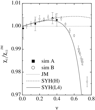
Figure 3: Density dependence of the ratio $\chi_{11}/\chi_{11}^{\text{JM}}$ for a hard-disk binary mixture with parameters as given in Table 1. The filled squares and open circles represent our simulation data A and B, respectively. The lines represent the ratio $\chi_{11}^{\text{SYH}}/\chi_{11}^{\text{JM}}$ for case B with $\chi(\nu)=\chi^{\text{H}}(\nu)$ (dashed line) and with $\chi(\nu)=\chi^{\text{L4}}(\nu)$ (solid line); the dotted line represents Eq. (8). The theoretical curves for case A are practically indistinguishable from those for case B and so they are not plotted.

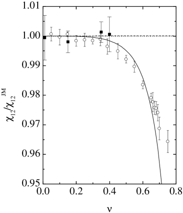
Figure 4: Same as in Fig. 3, except for $\chi_{12}/\chi_{12}^{\text{JM}}$.

Figure 5: Same as in Fig. 3, except for $\chi_{22}/\chi_{22}^{\text{JM}}$.

IV.1.1 Low densities

We observe that $\chi_{ij}^{\text{SYH}}/\chi_{ij}^{\text{JM}}$ with both prescriptions $\chi(\nu)=\chi^{\text{H}}(\nu)$ and $\chi(\nu)=\chi^{\text{L4}}(\nu)$ are practically indistinguishable up to $\nu\approx 0.3$. This is consistent with the fact that in that domain of low and moderate densities the correction (7) to Henderson’s EOS is irrelevant, as shown in Fig. 1. On the other hand, some limitations of Eq. (8) are already apparent in the range $0<\nu\lesssim 0.3$: the JM approximation (slightly) underestimates the small-small contact value ($\chi_{11}^{\text{JM}}<\chi_{11}$), while it overestimates the large-large contact value ($\chi_{22}^{\text{JM}}>\chi_{22}$). These two effects, which are not linked to the use of $\chi^{\text{H}}(\nu)$, are reasonably well captured by Eq. (II.2.2), as expected from (22). In the case of the cross contact value, we have $\chi_{12}\simeq\chi_{12}^{\text{JM}}$ for $0<\nu\lesssim 0.3$, in agreement with the fact that $z_{12}\simeq 1$ in our mixtures A and B.

IV.1.2 High densities

In the high-density domain $\nu\gtrsim 0.3$, the simulation data clearly deviate from both Eq. (8) and Eq. (II.2.2) when the latter is combined with $\chi(\nu)=\chi^{\text{H}}(\nu)$. Both theories tend to overestimate the contact values, what is essentially a trait inherited from Henderson’s EOS. On the other hand, a much better agreement is obtained when Eq. (II.2.2) is combined with Eq. (7) for the monodisperse fluid. The remaining deviations of the latter theory from the simulation values are a reflection of the approximate character of Eq. (II.2.2) rather than that of Eq. (7), in view of Fig. 1. Part of the deviations for the highest densities may be due to the proximity to crystallization. In the monodisperse case, it is known that the hard-disk fluid undergoes a freezing transition (possibly mediated by a hexatic phaseJ99 ) at an area fraction $\nu\simeq 0.7$.J99 ; Lu01 ; Lu01b ; Lu04 ; Lu02 ; kawamura79 In any case, polydispersity tends to increase the freezing transition density. For mixture A, our simulations indicate that the transition takes place between $\nu=0.75$ and $\nu=0.8$. For more details on very high densities in the mono- and bi-disperse situations see Refs. Lu01, and Lu02, , respectively.

IV.2 Equation of State

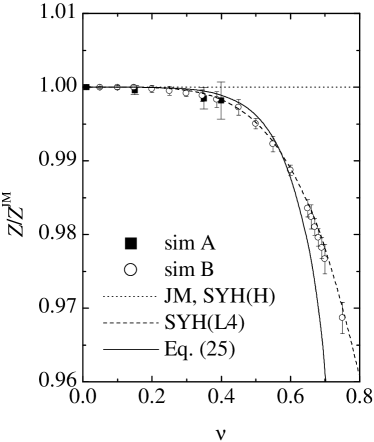
Figure 6: Density dependence of the ratio $Z/Z^{\text{JM}}$ for a hard-disk binary mixture with parameters as given in Table 1. The filled squares and open circles represent our simulation data A and B, respectively. The lines represent the ratio $Z^{\text{SYH}}/Z^{\text{JM}}$ for case B with $\chi(\nu)=\chi^{\text{H}}(\nu)$ (dotted line – unity) and $\chi(\nu)=\chi^{\text{L4}}(\nu)$ (solid line). The dashed line is the empirical relation (25) proposed in Ref. Lu01b, .

Although in this paper we have been mainly concerned with the contact values of the RDFs, it is worth considering the compressibility factor $Z\equiv p/\rho k_{B}T$. The simulation values of the ratio $Z/Z^{\text{JM}}$, where $Z^{\text{JM}}$ is given by Eq. (12) are plotted in Fig. 6. We observe that the JM EOS is fairly accurate for $\nu\lesssim 0.4$, even though the individual values $\chi_{ij}^{\text{JM}}$ are not that good in the same density range. This is mainly due to a fortunate “cancellation of errors” ($\chi_{11}^{\text{JM}}<\chi_{11}$, while $\chi_{22}^{\text{JM}}>\chi_{22}$). As a matter of fact, as already mentioned in Sec. II, the recipe (18) in combination with $\chi(\nu)=\chi^{\text{H}}(\nu)$ becomes identical with $Z^{\text{JM}}$. Nevertheless, the JM approximation again overestimates the simulation data for higher densities ($\nu\gtrsim 0.4$). When $\chi(\nu)=\chi^{\text{L4}}(\nu)$ is used, Eq. (18) becomes quite reasonable, although it slightly underestimates the mixture pressure of the fluid at the highest densities.

Interestingly, a recently proposed empirical correction to the EOS

$$Z=1+(1-a\nu^{4})\left(Z^{\text{JM}}-1\right),\quad a=0.1,$$ (25)

see Eq. (20) in Ref. Lu01b, , works also pretty well for the parameter set used here, however, without theoretical foundation. The excellent performance of Eq. (25) for $x_{1}\simeq 0.8$ and $\sigma_{1}/\sigma_{2}=\frac{1}{2}$ does not necessarily extend to other compositions. In fact, Eq. (25) is not as good as Eq. (7) in the monodisperse case.

V Conclusion

In this paper we have presented molecular dynamics results for the contact values $\chi_{ij}=g_{ij}(\sigma_{ij})$ of the radial distribution functions (RDFs) $g_{ij}(r)$ of binary mixtures of additive hard disks. As a representative case we have fixed mole fractions $x_{1}\simeq 0.8$ and $x_{2}\simeq 0.2$, and used a diameter ratio $\sigma_{1}/\sigma_{2}=\frac{1}{2}$. A set of numerical values of the area fraction $\nu$ have been considered, covering the dilute, the intermediate, and the dense regime.

The simulation results have been used to assess the reliability of theoretical expressions previously proposed in the literature. Until recently, practically the only proposal was the one by Jenkins and Mancini,JM87 which is expressed by Eq. (8). This approximation succeeds in capturing the main trends in the intricate dependence of $\chi_{ij}$ on the area fraction and the composition of the mixture, even at a quantitative level.

On the other hand, our simulation data expose some (small) limitations of $\chi_{ij}^{\text{JM}}$: already for low and moderate densities ($\nu\lesssim 0.3$) the JM recipe tends to underestimate the small-small correlation value and overestimate the large-large value; for higher densities ($\nu\gtrsim 0.3$), $\chi_{ij}^{\text{JM}}$ overestimates the correct values, an effect that can be traced back to the fact that $\chi_{ij}^{\text{JM}}$ is strongly tied to Henderson’s EOS.H75

These two shortcomings are widely corrected by a recent proposal made by Santos et al.,SYH02 Eq. (II.2.2). While $\chi_{ij}^{\text{JM}}$ is a linear function of the parameter $z_{ij}$ defined by Eq. (9), $\chi_{ij}^{\text{SYH}}$ is a quadratic function. This higher order approach allows $\chi_{ij}^{\text{SYH}}$ to satisfy an extra consistency condition in the limit of highly asymmetric mixtures.SYH02 Moreover, $\chi_{ij}^{\text{SYH}}$ can be used in conjunction with any desired expression for the contact value of the monodisperse fluid. When instead of Henderson’s expression the one recently proposed by one of usLu01 ; Lu02 is employed, $\chi_{ij}^{\text{SYH}}$ exhibits a reasonable agreement with the simulation data for $\nu\gtrsim 0.3$.

In spite of this, it can be observed that $\chi_{ij}^{\text{SYH}}$ tends to underestimate the simulation data for very high densities ($\nu\gtrsim 0.6$), so that an even better approximation is needed in that extreme, high density fluid regime. From this point of view, we hope that our simulation data will be helpful to test the accuracy of other future theoretical proposals that have been or will be made.

- (1) J.-P. Hansen and I.R. McDonald, Theory of Simple Liquids (Academic Press, London, 1986).
- (2) H. Löwen, Phys. Rep. 237, 249 (1994); C.N. Likos, Phys. Rep. 348, 267 (2001).
- (3) C.S. Campbell, Annu. Rev. Fluid Mech. 22, 57 (1990); I. Goldhirsch, ibid. 35, 267 (2003).
- (4) W.A. Steele, J. Chem. Phys. 65, 5256 (1976); E.D. Glandt, A.L. Myers, and D.D. Fitts, ibid. 70, 4243 (1979).
- (5) M. Brunner, C. Bechinger, U. Herz, and H.H. Grünberg, Europhys. Lett. 63, 791 (2003).
- (6) J.T. Jenkins and F. Mancini, J. Appl. Mech. 54, 27 (1987).
- (7) J.T. Willits and B.Ö. Arnarson, Phys. Fluids, 11, 3116 (1999).
- (8) M. Alam, J.T. Willits, B.Ö. Arnarson, and S. Luding, Phys. Fluids 14, 4085 (2002).
- (9) M. Alam and S. Luding, Gran. Matt. 4, 139 (2002).
- (10) M. Alam and S. Luding, J. Fluid Mech. 476, 69 (2003).
- (11) V. Garzó and J.M. Montanero, Phys. Rev. E 68, 041302 (2003).
- (12) V. Garzó and J.M. Montanero, Gran. Matt., 5, 165 (2003).
- (13) M.F. Rahaman, J. Naser, and P.J. Witt, Powder Technol. 138, 82 (2003).
- (14) S.R. Dahl, R. Clelland, and C.M. Hrenya, Powder Technol. 138, 7 (2003).
- (15) S.R. Dahl and C.M. Hrenya, Phys. Fluids 16, 1 (2004).
- (16) J.M. Montanero and V. Garzó, Mol. Sim. 29, 357 (2003).
- (17) J.H. Ferziger and G.H. Kaper, Mathematical Theory of Transport Processes in Gases (North–Holland, Amsterdam, 1972).
- (18) J.S. Rowlinson and F. Swinton, Liquids and Liquid Mixtures (Butterworth, London, 1982).
- (19) J.P. Noworyta, D. Henderson. S. Sokołowski, and K.-Y. Chan, Mol. Phys. 95, 415 (1998).
- (20) D. Henderson, F.F. Abraham, and J.A. Barker, Mol. Phys. 31, 1291 (1976).
- (21) A. Santos, S.B. Yuste, and M. López de Haro, J. Chem. Phys. 117, 5785 (2002).
- (22) D. Henderson, Mol. Phys. 30, 971 (1975).
- (23) L. Verlet and D. Levesque, Mol. Phys. 46, 969 (1982).
- (24) A. Santos, López de Haro, and S.B. Yuste, J. Chem. Phys. 101, 4622 (1995).
- (25) A. Mulero, F. Cuadros, and C. Galán, J. Chem. Phys. 107, 6887 (1997).
- (26) S. Luding, Phys. Rev. E 63, 042201 (2001).
- (27) S. Luding, Adv. Compl. Syst. 4, 379 (2002); reprinted in Challenges in Granular Physics, T. Halsey and A. Mehta, eds. (World Scientific, Singapore, 2002), pp. 91–100.
- (28) S. Luding, in The Physics of Granular Media, H. Hinrichsen and D. Wolf, eds. (Wiley, in press).
- (29) S. Luding and O. Strauß, in Granular Gases, T. Pöschel and S. Luding, eds. (LNP 564, Springer-Verlag, Berlin, 2001), pp. 389–409.
- (30) J.J. Erpenbeck and M. Luban, Phys. Rev. A 32, 2920 (1985).
- (31) A. Jaster, Phys. Rev. E 59, 2594 (1999); S. Sengupta, P. Nielaba, and K. Binder, ibid. 61, 6294 (2000); H. Watanabe, S. Yukawa, Y. Ozeki, and N. Ito, ibid. 66, 041110 (2002).
- (32) C. Barrio and J.R. Solana, J. Chem. Phys. 115, 7123 (2001); 117, 2451 (2002).
- (33) A. Santos, S.B. Yuste, and M. López de Haro, Mol. Phys. 96, 1 (1999).
- (34) M.P. Allen and D.J. Tildesley, Computer Simulation of Liquids (Oxford University Press, Oxford, 1987).
- (35) B.D. Lubachevsky, J. Comp. Phys. 94, 255 (1991).
- (36) H. Kawamura. Prog. Theor. Phys. 61, 1584 (1979).