Rosenfeld functional for non-additive hard spheres

Abstract

The fundamental measure density functional theory for hard spheres is generalized to binary mixtures of arbitrary positive and moderate negative non-additivity between unlike components. In bulk the theory predicts fluid-fluid phase separation into phases with different chemical compositions. The location of the accompanying critical point agrees well with previous results from simulations over a broad range of non-additivities and both for symmetric and highly asymmetric size ratios. Results for partial pair correlation functions show good agreement with simulation data.

Density-functional theory (DFT) is a powerful approach to study equilibrium properties of inhomogeneous systems, including dense liquids and solids of single- and multi-component substances [1]. Its practical applicability depends on the quality of the approximation to the central object, the (Helmholtz) excess free energy functional arising from the interparticle interactions. The specific model of additive hard sphere mixtures constitutes the reference system par excellence to describe mixtures governed by steric repulsion, and Rosenfeld’s fundamental-measure theory (FMT) [2, 3, 4, 5] is arguably the best available approximation to tackle inhomogeneous situations. A rapidly increasing number of applications to interesting physical problems can be witnessed [6].

The more general non-additive hard sphere mixture is defined through pair potentials between particles of species $i$ and $j$, given as $V_{ij}(r)=\infty$ for $r<\sigma_{ij}$ and 0 otherwise, where $r$ is the center-center distance between the two particles, and $\sigma_{ij}$ is the distance of minimal approach between particles of species $i$ and $j$. In a binary mixture non-additivity is measured conventionally through the parameter $\Delta=2\sigma_{12}/(\sigma_{11}+\sigma_{22})-1$. The physics of non-additive hard sphere mixtures is considerably richer than that of the additive case. In particular the case of $\Delta>0$ is striking, as small values of $\Delta$ are known to be already sufficient to induce stable fluid-fluid demixing into phases with different chemical compositions (for recent studies see e.g. references [7, 8, 9, 10]).

The treatment of general non-additivity is elusive in the FMT framework. The author is aware of successful studies only in four special cases: First, for the Asakura-Oosawa-Vrij (AOV) model [11, 12], where species 1 represents colloidal hard spheres and species 2 (with $\sigma_{22}=0$) represents non-interacting polymer coils with radius of gyration equal to $\sigma_{12}-(\sigma_{11}/2)$, an excess free energy functional was given [13]. Second, a free energy functional for the Widom-Rowlinson (WR) model, where $\sigma_{11}=\sigma_{22}=0$, was obtained [14]. Third, the depletion potential between two big spheres immersed in a sea of smaller spheres was obtained through “Roth’s trick” of working on the level of the one-body direct correlation functional [15, 16, 17]. In this case the functional for the additive case is sufficient to obtain results, but the approach is limited to small concentration of big spheres. Fourth, in Lafuente and Cuesta’s FMT for lattice hard core models, due the an odd-even effect of the particle sizes (measured in units of lattice constants), non-additivity of the size of one lattice spacing arises [18]. This effect, however, is specific to lattice models and vanishes in the continuum limit.

The aim of the present letter is to generalize FMT for hard spheres to the case of general positive and moderate negative non-additivity and arbitrary size asymmetry. The proposed extended framework accommodates, in the respective limits, the Rosenfeld functional for additive hard sphere mixtures [2], the DFT for the extreme non-additive AOV case [13], and the exact virial expansion up to second order in densities. The structure of the theory, however, goes qualitatively beyond that of either limit.

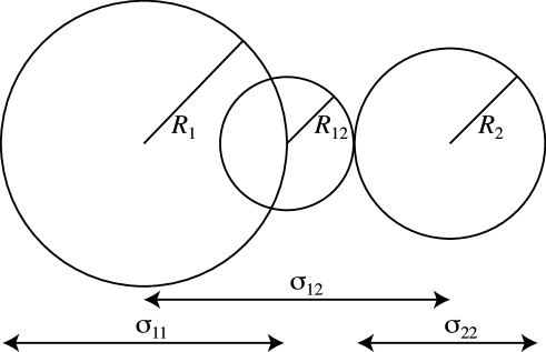
Figure 1: Illustration of the relevant length scales. The hard core interaction distances $\sigma_{ij}$ between pairs of particles of species $ij=11,12$ and 22 are related to radii through $\sigma_{11}=2R_{1}$, $\sigma_{12}=R_{1}+R_{12}+R_{2}$ and $\sigma_{22}=2R_{2}$, respectively. The spheres of radii $R_{1}$ and $R_{2}$ represent the weight functions $w_{\alpha}^{(1)}$ and $w_{\beta}^{(2)}$, respectively, and can be viewed as “true” particle shapes. The sphere of radius $R_{12}$ represents the kernel $K_{\alpha\beta}^{(12)}$ being a mere construct to generate the correct hard core distance $\sigma_{12}$ between species 1 and 2.

The excess (over ideal) Helmholtz free energy functional is expressed as

$$\quad{\mathcal{F}}_{\rm exc}[\rho_{1},\rho_{2}]=k_{B}T\int d{\bf x}d{\bf x}^{\prime}\sum_{\alpha,\beta=0}^{3}K^{(12)}_{\alpha\beta}(|{\bf x}-{\bf x}^{\prime}|)\Phi_{\alpha\beta}\left(\{n_{\nu}^{(1)}({\bf x})\},\{n_{\tau}^{(2)}({\bf x}^{\prime})\}\right),$$ (1)

where $\rho_{i}({\bf r})$ is the one-body density distributions of species $i=1,2$ dependent on position ${\bf r}$, $k_{B}T$ is the thermal energy, $\Phi_{\alpha\beta}$ for $\alpha,\beta=0,1,2,3$ is the free energy density depending on the sets of weighted densities $\{n_{\nu}^{(i)}\}$ for $i=1,2$, and the kernels $K_{\alpha\beta}^{(12)}(r)$ are a means to control the range of non-locality between unlike components and depend solely on distance $r$. The weighted densities are built in the usual way [2] through convolution of the respective bare density profile with appropriate weight functions:

$$n_{\nu}^{(i)}({\bf x})=\int d{\bf r}\rho_{i}({\bf r})w_{\nu}(|{\bf x}-{\bf r}|,R_{i}),\quad i=1,2,$$ (2)

where $\nu=0,1,2,3$ labels the type of weight function, and $R_{i}=\sigma_{ii}/2$ is the particle radius of species $i=1,2$. The (fully scalar) Kierlik-Rosinberg form [19, 20] of the $w_{\nu}(r,R)$ is used in the following, as this renders the determination of the $K_{\alpha\beta}^{(12)}(r)$ more straightforward. The $w_{\nu}(r,R)$ are

$$\eqalign{w_{0}&=-\delta^{\prime\prime}(R-r)/(8\pi)+\delta^{\prime}(R-r)/(2\pi r),\\ w_{1}&=\delta^{\prime}(R-r)/(8\pi),\\ w_{2}&=\delta(R-r),\\ w_{3}&=\Theta(R-r),}$$ (3)

where $R=R_{i}$, the prime denotes the derivative w.r.t. the argument, $\delta(\cdot)$ is the Dirac distribution, and $\Theta(\cdot)$ is the step function. Alternatively, in Fourier space the weight functions are $\tilde{w}_{\alpha}(k,R)=4\pi\int drw_{\alpha}(r,R)\sin(kr)r/k$ and given as

$$\eqalign{\tilde{w}_{0}&=c+(kRs/2),\\ \tilde{w}_{1}&=(kRc+s)/(2k),\\ \tilde{w}_{2}&=4\pi Rs/k,\\ \tilde{w}_{3}&=4\pi(s-kRc)/k^{3},}$$ (8)

with the abbreviations $s=\sin(kR)$ and $c=\cos(kR)$. The kernels $K_{\alpha\beta}^{(12)}(r)$ in (1) can be viewed as $\alpha\beta$-components of a second-rank tensor

$$\hat{\bf K}^{(12)}(r)=\left(\begin{tabular}[]{cccc}$w_{3}$&$w_{2}$&$w_{1}$&$w_{0}$\\ $w_{2}$&$w_{1}^{\dagger}$&$w_{0}^{\dagger}$&$w_{-1}$\\ $w_{1}$&$w_{0}^{\dagger}$&$w_{-1}^{\dagger}$&$w_{-2}$\\ $w_{0}$&$w_{-1}$&$w_{-2}$&$w_{-3}$\end{tabular}\right),\\$$ (9)

where indexing is such that the top row contains $K_{00}^{(12)},\ldots,K_{03}^{(12)}$, etc, and ${\dagger}$ distinguishes different elements. All $K_{\alpha\beta}^{(12)}(r)$ possess a range of $R_{12}=\sigma_{12}-(\sigma_{11}+\sigma_{22})/2$, i.e. vanish for values of $r$ beyond that distance (see figure 1 for an illustration of the length scales). The dimension of $K_{\alpha\beta}^{(12)}$ is $(\rm length)^{-\alpha-\beta}$, and hence the dimension of $w_{\gamma}$ is $(\rm length)^{\gamma-3}$. The elements of $\hat{\bf K}^{(12)}$ are defined, with $R=R_{12}>0$, through (3), and furthermore

$$\eqalign{w_{1}^{\dagger}&=\delta^{\prime}(R-r),\\ w_{0}^{\dagger}&=\delta^{\prime\prime}(R-r)/(8\pi),\\ w_{-1}^{\dagger}&=\delta^{(3)}(R-r)/(64\pi^{2}),\\ w_{-1}&=\delta^{{}^{\prime\prime}}(R-r)/(2\pi r)-\delta^{(3)}(R-r)/(8\pi),\\ w_{-2}&=\delta^{(3)}(R-r)/(16\pi^{2}r)-\delta^{(4)}(R-r)/(64\pi^{2}),\\ w_{-3}&=-\delta^{(4)}(R-r)/(8\pi^{2}r)+\delta^{(5)}(R-r)/(64\pi^{2}),}$$ (16)

with the derivatives $\delta^{(\gamma)}(x)=d^{\gamma}\delta(x)/dx^{\gamma}$ for $\gamma=3,4,5$. Again we also give the Fourier space representation [being together with (8) also valid for $R=R_{12}<0$], which reads

$$\eqalign{\tilde{w}_{1}^{\dagger}&=4\pi(kRc+s)/k,\\ \tilde{w}_{0}^{\dagger}&=c-(kRs/2),\\ \tilde{w}_{-1}^{\dagger}&=-(k^{2}Rc+3ks)/(16\pi),\\ \tilde{w}_{-1}&=(k^{2}Rc-ks)/2,\\ \tilde{w}_{-2}&=-k^{3}Rs/(16\pi),\\ \tilde{w}_{-3}&=(k^{4}Rc-3k^{3}s)/(16\pi).}$$ (23)

In order to express the dependence of the free energy density, $\Phi_{\alpha\beta}$ in equation (1), on the weighted densities (2) we introduce ansatz functions $A_{\alpha\gamma}^{(i)}$ for species $i=1,2$ that possess the dimension of $(\rm length)^{\alpha-3}$ and the order $\gamma$ in density (i.e. contain $\gamma$ factors $n_{\tau}^{(i)}$). Explicit expressions for the non-vanishing terms are

$$A_{01}^{(i)}=n_{0}^{(i)},\quad A_{02}^{(i)}=n_{1}^{(i)}n_{2}^{(i)},\quad A_{03}^{(i)}=\left(n_{2}^{(i)}\right)^{3}/(24\pi),$$ (24)

$$A_{11}^{(i)}=n_{1}^{(i)},\quad A_{12}^{(i)}=\left(n_{2}^{(i)}\right)^{2}/(8\pi),\quad A_{21}^{(i)}=n_{2}^{(i)},\quad A_{30}^{(i)}=1.$$ (25)

The excess free energy density is then constructed as

$$\Phi_{\alpha\beta}=\sum_{\gamma=0}^{6}\sum_{\gamma^{\prime}=0}^{3}A_{\alpha\gamma^{\prime}}^{(1)}A_{\beta(\gamma-\gamma^{\prime})}^{(2)}\varphi_{\rm 0d}^{(\gamma)}\left(n_{3}^{(1)}+n_{3}^{(2)}\right),$$ (26)

where $\varphi_{0d}^{(\gamma)}(\eta)\equiv d^{\gamma}\varphi_{0d}(\eta)/d\eta^{\gamma}$ is the $\gamma$th derivative of the zero-dimensional excess free energy as a function of the average occupation number $\eta$ [3], $\varphi_{0d}(\eta)=(1-\eta)\ln(1-\eta)+\eta$, and $\varphi_{0d}^{(0)}(\eta)\equiv\varphi_{0d}(\eta)$ for $\gamma=0$. The specific form (26) ensures both that the terms in the sum in (1) possesses the correct dimension of $(\rm length)^{-6}$ and that the prefactor of $\varphi_{\rm 0d}^{(\gamma)}$ in (26) is of the total order $\gamma$ in densities, as is common in FMT. This completes the prescription for the functional; a full account of all details, also for multi-component mixtures and for lower spatial dimensionality, will be given elsewhere.

Here we discuss some of the properties of the theory. For small densities it is straightforward to show that the correct virial expansion up to second order in densities is obtained, $F_{\rm exc}\to-\sum_{ij}\int d^{3}rd^{3}r^{\prime}f_{ij}(|{\bf r}-{\bf r}^{\prime}|)\rho_{i}({\bf r})\rho_{j}({\bf r}^{\prime})/2$, where the Mayer functions, $f_{ij}(r)=\exp(-V_{ij}(r)/(k_{B}T))-1$, are recovered through

$$f_{12}=-\sum_{\alpha\beta=0}^{3}w_{\alpha}^{(1)}\ast K_{\alpha\beta}^{(12)}\ast w_{\beta}^{(2)},\quad f_{ii}=-\sum_{\alpha=0}^{3}w_{\alpha}^{(i)}\ast w_{3-\alpha}^{(i)},\;i=1,2,$$ (27)

where $\ast$ denotes the convolution, $g({\bf r})\ast h({\bf r})=\int d^{3}r^{\prime}g({\bf r}^{\prime})h({\bf r}-{\bf r}^{\prime})$. In the limit of an additive mixture, $\Delta\to 0$ and hence $R_{12}\to 0$, one finds that $K_{\alpha\beta}(x)\to 0$ if $\beta\neq 3-\alpha$ and $K_{\alpha(\alpha-3)}(x)\to\delta(x)$ otherwise. This leads to a cancellation of one spatial integration in (1) and yields the Rosenfeld functional for a binary additive hard sphere mixture [2] with radii $R_{1}$ and $R_{2}$. In the AOV limit, $R_{2}\to 0$, one finds that $n_{\alpha}^{(2)}\to 0$ if $\alpha\neq 0$, and $n_{0}^{(2)}\to\rho_{2}$ otherwise. The integration over ${\bf x}^{\prime}$ in (1) together with the kernel $K_{\alpha\beta}(|{\bf x}-{\bf x}^{\prime}|)$ and the fact that the density $n_{0}^{(2)}({\bf x}^{\prime})=\rho_{2}({\bf x}^{\prime})$ appears linearly in $\Phi_{\alpha\beta}$, see $A_{01}^{(2)}$ in (24), plays the same role that building weighted densities for the polymer species in the AOV case does. The resulting functional is equal to that for the AOV model [13]. However, in the WR limit, in contrast to [14], terms higher than on the second virial level vanish. For $\Delta=-1$ the two species decouple, and ${\cal F}_{\rm exc}[\rho_{1},\rho_{2}]={\cal F}_{\rm exc}[\rho_{1}]+{\cal F}_{\rm exc}[\rho_{2}]$ which is not obeyed by the present approximation, limiting its applicability to small values of $\Delta<0$.

We next turn to an investigation of bulk properties of the theory. To assess structure, direct correlation functions can be obtained via

$$c_{ij}^{(2)}(|{\bf r}-{\bf r}^{\prime}|)=\left.-\frac{\delta^{2}\beta{\mathcal{F}}_{\rm exc}}{\delta\rho_{i}({\bf r})\delta\rho_{j}({\bf r}^{\prime})}\right|_{\rho_{1},\rho_{2}=\rm const},$$ (28)

which can be shown to feature Percus-Yevick (PY) like behavior: $c_{ij}^{(2)}(r>\sigma_{12})=0$. Inverting the Ornstein-Zernike (OZ) relations permits to calculate partial structure factors, $S_{ij}(k)$, and partial pair correlation functions, $g_{ij}(r)$. We have carried out Monte Carlo (MC) computer simulations in the canonical ensemble with 1024 particles and $10^{5}$ MC moves per particle; histograms of all distances between particles yield benchmark results for $g_{ij}(r)$. We have chosen an intermediate size ratio of $\sigma_{22}/\sigma_{11}=0.5$ and have considered various values of $\Delta$ from $-0.3$ to 0.5 and a range of statepoints characterized by packing fractions, $\eta_{i}=\pi\rho_{i}\sigma_{ii}^{3}/6$ for $i=1,2$. For $\Delta=0$, the current DFT reproduces the solution of the PY integral equation, as the functional reduces to the Rosenfeld case, which is known to yield the same $c_{ij}^{(2)}(r)$ as the PY approximation. Results for the representative case $\Delta=0.2$ at two different statepoints are shown in figure 2. The core condition, $g_{ij}(r<\sigma_{ij})=0$, is only approximately fulfilled, but the overall agreement between results from theory and simulation is quite remarkable.

Figure 2: Partial pair correlation functions, $g_{ij}(r)$, between species $ij=11,12$ and 22 (as indicated), as a function of the scaled distance $r/\sigma_{11}$, as obtained from the present DFT using the OZ route (dashed lines) and from MC simulation (solid lines). Results for $g_{12}$ ($g_{22}$) are shifted upwards by one (two) units for clarity. Parameters are $\sigma_{22}/\sigma_{11}=0.5$, $\Delta=0.3$, $\eta_{2}=\eta_{1}/8$ and $\eta_{1}=0.05$ (lower), 0.1 (upper). For comparison, the theoretical critical point is located at $\eta_{1}=0.118,\eta_{2}=0.0321$.

In principle one could envisage that this approach permits to study the depletion potential, $V_{\rm depl}^{(11)}(r)$, between particles of species 1 being generated by the immersion into a “sea” of particles 2 through $V_{\rm depl}^{(11)}(r)=-k_{B}T\ln g_{11}(r)$ for $\rho_{1}\to 0$, and $\rho_{2}=\rm const$. However, for the (relevant) case of small size ratios (e.g. $\sigma_{22}/\sigma_{11}\sim 0.1$, see [15, 16]) already in both limits of additive hard spheres and the AOV model the results are only of rather moderate accuracy, underestimating the strength of the depletion attraction [13], similar to results from the PY approximation. However, results from the present theory obtained through the OZ route (not shown) cross over smoothly between the additive hard sphere case and the AOV case, similar to the correct behavior [15, 16]. Hence one can conclude that the pair structure predicted by the current DFT is similar to that of the PY approximation. This is a remarkable property, and one can anticipate test-particle calculations to yield superior results.

Evaluating (1) at constant density fields yields an analytic expression for the bulk excess free energy for fluid states, $F_{\rm exc}={\cal F}_{\rm exc}[\rho_{1}{\rm=const},\rho_{2}{\rm=const}]$. The total Helmholtz free energy is then $F=F_{\rm exc}+k_{B}TV\sum_{i=1,2}\rho_{i}[\ln(\rho_{i}\Lambda_{i}^{3})-1]$, where $\Lambda_{i}$ is the (irrelevant) de Broglie wavelength of species $i$, and $V$ is the system volume. Via Taylor expanding $F_{\rm exc}$ in both densities one can show that it features the exact second virial coefficients (consistent with the correct incorporation of $f_{ij}(r)$ on the second virial level) and also the exact third virial coefficients (see e.g. [7]) provided $2\sigma_{12}>\max(\sigma_{11},\sigma_{22})$.

The fluid-fluid demixing spinodal can be obtained from (numerical) solution of $|\partial^{2}(F/V)/\partial\rho_{i}\partial\rho_{j}|=0$, and the location of the critical point can be determined from minimizing one of the chemical potentials, $\mu_{1}$ or $\mu_{2}$, along the spinodal. Such results are compared in figure 3 to those from simulations for $\sigma_{11}=\sigma_{22}$, performed in the semi-grand ensemble by Jagannathan and Yethiraj [10] and by Góźdź [9], the latter study including a finite size analysis, for a variety of non-additivities ranging from $\Delta=0.1-1$. For the highly asymmetric case of $\sigma_{22}=\sigma_{11}$ results from Gibbs ensemble simulations were obtained by Dijkstra [7]. For both size ratios the strong decrease of the total critical packing fraction with increasing values of $\Delta$, as well as the overall functional dependence are very well described by the theory. However, the precise value at given $\Delta$ is underestimated. This behavior is not uncommon for mean-field like theories and is also present in the AOV case.

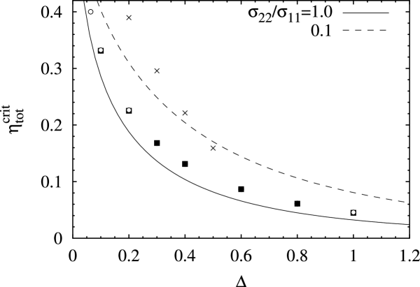
Figure 3: The total packing fraction at the critical point, $\eta_{\rm tot}^{\rm crit}$, where $\eta_{\rm tot}=\eta_{1}+\eta_{2}$, for a non-additive binary hard sphere mixture as a function of the non-additivity parameter $\Delta$. Shown are results from the present DFT (lines) and from simulations (symbols) for the symmetric case, $\sigma_{22}/\sigma_{11}=1$, by Góźdź [9] (filled squares) and by Jagannathan and Yethiraj [10] (open circles), as well as for the highly asymmetric case of $\sigma_{22}/\sigma_{11}=0.1$ by Dijkstra [7] (crosses).

A benefit of working on the level of the density functional is that the structure is consistent with the free energy. In figure 4 partial structure factors are shown for a range of values of $\Delta$ evaluated at the fluid-fluid critical point obtained from the free energy, and indeed $S_{ij}(k\to 0)\to\pm\infty$.

Figure 4: Partial structure factors, $S_{ij}(k)$ for $ij=11,12,22$ (as indicated), as a function of $k\sigma_{11}$ at the fluid-fluid critical point for size ratio $\sigma_{22}/\sigma_{11}=0.1$ and non-additivity $\Delta=0.2,0.5,1$. The results for $\Delta=0.5$ (1) are shifted upwards by 5 (10) units for clarity.

In conclusion, having demonstrated the good accuracy of the predictions of the current theory for bulk fluid properties of the non-additive hard sphere mixture, we are confident that it is well suited to study interesting and relevant interfacial situations, like the structure and tension of interfaces between demixed phases, wetting at substrates [21] and more. Note that any colloidal mixtures interacting with soft repulsive forces, as e.g. present in charge-stabilized dispersions, can be mapped (e.g. by the Barker-Henderson procedure) onto an effective non-additive hard sphere system. Hence one can anticipate experimental consequences of the structure and phase separation predicted by the present theory. The treatment of freezing [8] requires additional contributions to the free energy functional [3, 4].
H. Löwen, R. Evans, R. Blaak and K. Jagannathan are thanked for useful comments. Support by the SFB TR6 of the DFG is acknowledged. This work is part of the research program of FOM, that is financially supported by the NWO.

References

References

[1]
R. Evans, in Fundamentals of Inhomogeneous Fluids, edited by D.
Henderson (Dekker, New York, 1992), Chap. 3, p. 85.
[2]
Y. Rosenfeld, Phys. Rev. Lett. 63, 980 (1989).
[3]
Y. Rosenfeld, M. Schmidt, H. Löwen, and P. Tarazona, Phys. Rev. E 55,
4245 (1997).
[4]
P. Tarazona, Phys. Rev. Lett. 84, 694 (2000).
[5]
J. A. Cuesta, Y. Martinez-Raton, and P. Tarazona, J. Phys.: Condens. Matter
14, 11965 (2002).
[6]
See e.g. the special issue on DFT of liquids, J. Phys.: Condens. Matt. 14(46) 2002.
[7]
M. Dijkstra, Phys. Rev. E 58, 7523 (1998).
[8]
A. A. Louis, R. Finken, and J. P. Hansen, Phys. Rev. E 61, R1028
(2000).
[9]
W. T. Góźdź, J. Chem. Phys. 119, 3309 (2003).
[10]
K. Jagannathan and A. Yethiraj, J. Chem. Phys. 118, 7907 (2003).
[11]
S. Asakura and F. Oosawa, J. Chem. Phys. 22, 1255 (1954).
[12]
A. Vrij, Pure and Appl. Chem. 48, 471 (1976).
[13]
M. Schmidt, H. Löwen, J. M. Brader, and R. Evans, Phys. Rev. Lett. 85, 1934 (2000).
[14]
M. Schmidt, Phys. Rev. E 63, 010101(R) (2001).
[15]
R. Roth and R. Evans, Europhys. Lett. 53, 271 (2001).
[16]
R. Roth, R. Evans, and A. A. Louis, Phys. Rev. E 64, 051202 (2001).
[17]
A. A. Louis and R. Roth, J. Phys.: Condens. Matter 13, L777 (2001).
[18]
L. Lafuente and J. A. Cuesta, J. Phys.: Condens. Matter 14, 12079
(2002).
[19]
E. Kierlik and M. L. Rosinberg, Phys. Rev. A 42, 3382 (1990).
[20]
S. Phan, E. Kierlik, M. L. Rosinberg, B. Bildstein, and G. Kahl, Phys. Rev. E
48, 618 (1993).
[21]
J. M. Brader, R. Evans, M. Schmidt, and H. Löwen, J. Phys.: Condens.
Matter 14, L1 (2002).