Competition and adaptation in an Internet evolution model

Abstract

We model the evolution of the Internet at the Autonomous System level as a process of competition for users and adaptation of bandwidth capability. We find the exponent of the degree distribution as a simple function of the growth rates of the number of autonomous systems and the total number of connections in the Internet, both empirically measurable quantities. This fact place our model apart from others in which this exponent depends on parameters that need to be adjusted in a model dependent way. Our approach also accounts for a high level of clustering as well as degree-degree correlations, both with the same hierarchical structure present in the real Internet. Further, it also highlights the interplay between bandwidth, connectivity and traffic of the network.

A statistical physics approach to Internet modeling will be successful only if its large-scale properties can be explained and predicted on the basis of the interactions between basic units at the microscopic level Pastor-Satorras and Vespignani (2004); Dorogovtsev and Mendes (2003). Dynamical evolution rules acting at the local scale would then determine the behavior and the emergent structural properties of the whole Internet, which self-organizes under an absolute lack of centralized control Albert and Barabási (2002); Dorogovtsev and Mendes (2002). This approach is at the core of a set of recent network models focusing on evolution, which recognise growth as one of the key mechanisms on network formation, along with preferential attachment or other utility rules Barabási and Albert (1999); Huberman and Adamic (1999); Goh et al. (2002); Capocci et al. (2001); Fayed et al. (2003); Zhou et al. (2002). While several of such models succeed in depicting some of the Internet features, none of them accounts for a complete description of the real topology Faloutsos et al. (1999); Pastor-Satorras et al. (2001); Vázquez et al. (2002a). In this paper, we present a new growing network model which, from competition and adaptation mechanisms, reproduces the topological properties observed in the autonomous system level maps of the Internet, namely: i) a scale-free distribution of the number of connections –or degree– of vertices $k_{i}$, characterized by a power law $P(k)\sim k^{-\gamma}$, $2.1\leq\gamma<2.5$, ii) high clustering coefficient $c_{k}$, defined as the ratio between the number of connected neighbors of a node of degree $k$ and the maximum possible value averaged for all nodes of degree $k$, and, finally, iii) disassortative degree-degree correlations, quantified by means of the average nearest neighbors degree of nodes of degree $k$, $\bar{k}_{nn}(k)$ Pastor-Satorras et al. (2001).

We start our analysis by looking at the growth of the Internet during the last three decades. We focus on the temporal evolution of the number of hosts present in the Internet Hosts as compared to the number of distinct autonomous systems (ASs) and the total number of connections among them. We have reanalysed AS maps collected by the Oregon route-views project which has recorded the Internet topology at the AS level since November 1997 Evolution . Let $W(t)$, $N(t)$ and $E(t)$ be the total number of hosts (we assume that number of hosts is equivalent to number of users), number of ASs and edges among ASs at time $t$ respectively. Fig.1 shows empirical measurements for these quantities revealing exponential growths, $W(t)\sim W_{0}e^{\alpha t}$, $N(t)\sim N_{0}e^{\beta t}$ and $E(t)\sim E_{0}e^{\delta t}$ respectively, with rates $\alpha=0.036$, $\beta=0.029$ and $\delta=0.033$, where $\alpha\gtrsim\delta\gtrsim\beta$. These exponential growths, in turn, determine the scaling relations with the system size, that is, $W\sim N^{\alpha/\beta}$, $E\sim N^{\delta/\beta}$ and $\langle k\rangle\sim N^{\delta/\beta-1}$ Dorogovtsev and Mendes (2001). All three rates are, indeed, quite close to each other. This result poses the question of whether these inequalities actually hold or, in contrast, are due to statistical fluctuations. A simple argument will convince us that the inequalities are, actually, the natural answer. There are two mechanisms capable to compensate an increase in the number of users: the creation of new ASs and the creation of new connections by old ASs. When both mechanisms take place simultaneously, the rate of growth of new ASs, $\beta$, must necessarily be smaller than $\alpha$, whereas the rate of growth of the number of connections, $\delta$, must be greater than $\beta$. Any other situation would lead to an imbalance between the number of users and the maximum number of users that the system can manage.

Our model is defined according to the following rules: (i) At rate $\alpha W(t)$, new users joint the system and choose provider $i$ according to some preference function, $\Pi_{i}(\{\omega_{j}(t)\})$, where $\omega_{j}(t)$, $j=1,\cdots,N(t)$, is the number of hosts connected to AS $j$ at time $t$. The function $\Pi_{i}(\{\omega_{j}(t)\})$ is normalised so that $\sum_{i}\Pi_{i}(\{\omega_{j}(t)\})=1$ at any time. (ii) At rate $\beta N(t)$, new ASs join the network with an initial number of users, $\omega_{0}$, randomly withdrawn from the pool of users already attached to existing ASs. Therefore, $\omega_{0}$ can be understood as the minimum number of users required to keep ASs in business. (iii) At rate $\lambda$, each user changes his provider and chooses a new one using the same preference function $\Pi_{i}(\{\omega_{j}(t)\})$. Finally, (iv) each node tries to adapt its number of connections to other nodes according to its present number of users, in an attempt to provide them an adequate access to the Internet. We will discuss this last point in the second part of the work. With the above ingredients, in the continuum approximation, the dynamics of single nodes is described by the stochastic differential equation

$$\frac{d\omega_{i}}{dt}=A(\omega_{i},t)+\left[D(\omega_{i},t)\right]^{1/2}\xi(t),$$ (1)

where $A(\omega_{i},t)$ is a time dependent drift given by

$$A(\omega_{i},t)=(\alpha+\lambda)W(t)\Pi_{i}-\lambda\omega_{i}-\beta\omega_{0}$$ (2)

and the diffusion term by

$$D(\omega_{i},t)=(\alpha+\lambda)W(t)\Pi_{i}+\lambda\omega_{i}+\beta\omega_{0}-2\lambda\omega_{i}\Pi_{i}.$$ (3)

Application of the Central Limit Theorem guaranties the convergence of the noise $\xi(t)$ to a gaussian white noise in the limit $W(t)\gg 1$. The first term in the right hand side in Eq. (2) is a creation term accounting for new and old users that choose node $i$ as a provider. The second term represent those users who decide to change their providers and, finally, the last term corresponds to the decrease of users due to introduction of newly created ASs. To proceed further, we need to specify the preference function $\Pi_{i}(\{\omega_{j}(t)\})$. We assume that, as a result of a competition process, bigger ASs get users more easily than small ones. The simplest function satisfying this condition corresponds to the linear preference, that is,

$$\Pi_{i}(\{\omega_{j}(t)\})=\frac{\omega_{i}}{W(t)}$$ (4)

where $W(t)=\omega_{0}N_{0}\exp{(\alpha t)}$. In this case, the stochastic differential equation (1) reads

$$\frac{d\omega_{i}}{dt}=\alpha\omega_{i}-\beta\omega_{0}+\left[(\alpha+2\lambda)\omega_{i}+\beta\omega_{0}\right]^{1/2}\xi(t).$$ (5)

Notice that reallocation of users (i.e. the $\lambda$-term) only increases the diffusive part in Eq. (5) but has no net effect in the drift term, which is, eventually, the leading term. The complete solution of this problem requires to solve the Fokker-Plack equation corresponding to Eq. (5) with a reflecting boundary condition at $\omega=\omega_{0}$ and initial conditions $p(\omega_{i},t_{i}|\omega_{0},t_{i})=\delta(\omega_{i}-\omega_{0})$ ($\delta(\cdot)$ stands for the Dirac delta function). Here $p(\omega_{i},t|\omega_{0},t_{i})$ is the probability that node $i$ has wealth $\omega_{i}$ at time $t$ given that it had $\omega_{0}$ at time $t_{i}$. The choice of a reflecting boundary condition at $\omega=\omega_{0}$ is equivalent to assume that $\beta$ is the overall growth rate of the number of nodes, that is, the composition of the birth and dead processes ruling the evolution of the number of nodes.

Finding the solution for this problem is not an easy task. Fortunately, we can take advantage of the fact that, when $\alpha>\beta$, the average number of users of each node increases exponentially and, since $D(\omega_{i},t)={\cal O}\left(A(\omega_{i},t)\right)$, fluctuations vanishes in the long time limit. Under this zero noise approximation, the number of hosts connected to an AS introduced at time $t_{i}$ is

$$\omega_{i}(t|t_{i})=\frac{\beta}{\alpha}\omega_{0}+(1-\frac{\beta}{\alpha})\omega_{0}e^{\alpha(t-t_{i})}.$$ (6)

The probability density function of $\omega$ can be calculated in the long time limit as

$$p(\omega,t)=\beta e^{-\beta t}\int_{0}^{t}e^{\beta t_{i}}\delta(\omega-\omega_{i}(t|t_{i}))dt_{i}$$ (7)

which leads to

$$p(\omega,t)=\displaystyle{\frac{\tau(1-\tau)^{\tau}\omega_{0}^{\tau}}{(\omega-\tau\omega_{0})^{1+\tau}}\Theta(\omega_{c}(t)-\omega)},$$ (8)

where we have defined $\tau\equiv\beta/\alpha$ and the cut-off is given by $\omega_{c}(t)\sim(1-\tau)\omega_{0}e^{\alpha t}\sim W(t)$. Thus, in the long time limit, $p(\omega,t)$ approaches a stationary distribution with an increasing cut-off. In the case of the Internet, $\alpha\gtrsim\beta$ which implies an exponent smaller but close to 2. A similar result was obtained in Fayed et al. (2003).

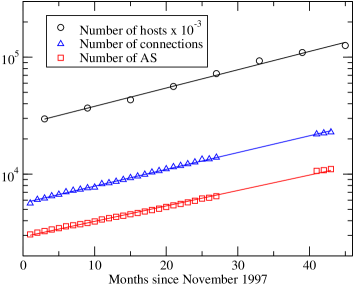
Figure 1: Temporal evolution of the number of hosts, autonomous systems and connections among them from November 1997 to May 2002. Solid lines are the best fit estimates which gives the values for the rate growths of $\alpha=0.036$, $\beta=0.029$ and $\delta=0.033$ (units are month^-1).

The key point in what follows is how to relate the number of users attached to an AS with its degree. Our basic assumption is that vertices are continuously adapting their bandwidth to the number of users they have. However, once an AS decides to increase its bandwidth it has to find a peer who, at the same time, wants to increase its bandwidth as well. The reason is that connection costs among ASs must be assumed by both peers. This fact differs from other growing models in which vertices do not ask target vertices if they really want to form those connections. Our model is, then, to be though of as a coupling between a competition process for resources and adaptation of vertices to their current situation, with the constraint that connections are only formed between active nodes. Let $b_{i}(t|t_{i})$ be the total bandwidth of an AS at time $t$ given that it was introduced at time $t_{i}$. This quantity can include single connections with other ASs, i. e. the topological degree $k$, but it also accounts for connections which have higher capacity. This is equivalent to say that the network is, in fact, weighted and $b_{i}$ is the weighted degree. To simplify the model we consider that bandwidth is discretized in such a way that single connections with high capacity are equivalent to multiple connections between the same ASs. Then, when a pair of ASs agrees to increase their mutual connectivity the connection is newly formed if they were not previously connected or, if they were, their mutual bandwidth increases by one unit. Now, we assume that, at time $t$, each AS adapts its total bandwidth proportionally to its number of users. We can write

$$b_{i}(t|t_{i})=1+a(t)\left(\omega_{i}(t|t_{i})-\omega_{0}\right).$$ (9)

Summing Eq. (9) for all nodes we get

$$a(t)=\frac{2B(t)-N(t)}{W(t)-\omega_{0}N(t)}\sim\frac{2B(t)}{W(t)},$$ (10)

where $B(t)$ is the total bandwidth of the network which is, obviously, an upper bound to the total number of edges of the network. This suggests that $B(t)$ will grow according to $B(t)=B_{0}e^{\delta^{\prime}t}$, where $\delta^{\prime}\gtrsim\delta$. Using this assumption, we can express the individual bandwidth as $b_{i}(t|t_{i})\sim N(t)^{(\delta^{\prime}-\alpha)/\beta}\omega_{i}(t|t_{i})$. From this equation, the scaling of the maximum bandwidth with the system size reads $b_{c}(t)\sim N(t)^{\delta^{\prime}/\beta}$, that is, faster than $N(t)$. This implies that the network must necessarly contain multiple connections. Then, we propose that degree and bandwidth are related, in a statistical sense, through the following scaling relation

$$k(t|t_{i})\sim\left[b(t|t_{i})\right]^{\mu},$$ (11)

where the scaling exponent, $\mu<1$, is obtained by imposing that the maximum degree scales linearly with $N(t)$ . This sets the scaling exponent to $\mu=\beta/\delta^{\prime}$. All four growth rates in the model are not independent but can be related by exploring the interplay between bandwidth, connectivity and traffic of the network. As the number of users grow, the global traffic of the Internet also grows, which means that ASs do not only adapt their bandwidth to their number of users but to the global traffic of the network. Therefore, $a(t)$ must be an increasing function of $t$, which, in turn, implies that $\delta^{\prime}>\alpha$. Using this condition and summing Eq. (11) for all vertices, the scaling of the total number of connections is $E(t)\sim N(t)^{2-\alpha/\delta^{\prime}}$, which leads to $\delta^{\prime}=\alpha\beta/(2\beta-\delta)$. Combining this relation with Eqs. (8), (9) and (11), the degree distribution reads

$$P(k)\sim\frac{\tau(1-\tau)^{\tau}\left[\omega_{0}a(t)\right]^{\tau}}{\mu}\frac{1}{k^{\gamma}}\Theta(k_{c}(t)-k),$$ (12)

where the exponent $\gamma$ takes the value

$$\gamma=1+\frac{\beta}{2\beta-\delta}.$$ (13)

Strikingly, the exponent $\gamma$ has lost any dependence on $\alpha$ becoming a function of the growth rate of both the number of ASs and the number of connections of the network. Using the empirical values for $\beta$ and $\delta$, the predicted exponent is $\gamma=2.2\pm 0.1$, in excellent agreement with the values reported in the literature Faloutsos et al. (1999); Pastor-Satorras et al. (2001); Vázquez et al. (2002a).

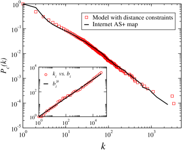
Figure 2: Cumulative degree distribution ($P_{c}(k)=\sum_{k}P(k^{\prime})$) for the extended AS map compared to simulations of the model, $r=0.8$. Inset: AS’s degree as a function of AS’s bandwidth. The solid line stands for the scaling relation Eq. (11) with $\mu=\beta/\delta^{\prime}=0.75$.

So far, we have been mainly interested in the degree distribution of the AS map but not in the specific way in which the network is formed. To fill this gap we have performed numerical simulations that generate network topologies in nice agreement with real measures of the Internet that go beyond the degree distribution. We consider a realistic geographical deployment of ASs and physical distance among them to take into account connection costs Yook et al. (2002). Our algorithm, following the lines of the model, works in four steps:

1. At iteration t, $\Delta W(t)=\omega_{0}N_{0}(e^{\alpha t}-e^{\alpha(t-1)})$ users join the network and choose provider among the existing nodes using the preference rule Eq. (4).

2. $\Delta N(t)=N_{0}(e^{\beta t}-e^{\beta(t-1)})$ new ASs are introduced with $\omega_{0}$ users each, those being randomly withdrawn from already existing ASs. Newly created ASs are located in a two dimensional plane following a fractal set of dimension $D_{f}=1.5$ Yook et al. (2002).

3. Each AS evaluate its increase of bandwidth, $\Delta b_{i}(t|t_{i})$, according to Eq. (9).

4. A pair of nodes, $(i,j)$, is chosen with probability proportional to $\Delta b_{i}(t|t_{i})$ and $\Delta b_{j}(t|t_{j})$ respectively, and, whenever they both need to increase their bandwidth, they form a connection with probability $D(d_{ij},\omega_{i},\omega_{j})$. This function takes into consideration that, due to connection costs, physical links over long distances are unlikely to be created by small peers. Once the first connection has been formed, they create a new connection with probability $r$, whenever they still need to increase their bandwidth. This step is repeated until all nodes have the desired bandwidth.

It is important to stress the fact that nodes must be chosen with probability proportional to their increase in bandwidth at each step. The reason is that those nodes that need a high bandwidth increase will be more active when looking for partners to whom form connections. Another important point is the role of the parameter $r$. This parameter takes into account the balance between the costs of forming connections with new peers and the need for diversification in the number of partners. The effect of $r$ in the network topology is to tune the average degree and the clustering coefficient by creating more multiple connections. The exponent of the degree distribution is unaffected except in the limiting case $r\rightarrow 1$. In this situation, big peers will create a huge amount of multiple connections among them, reducing, thus, the maximum degree of the network. Finally, we chose an exponential form for the distance probability function $D(d_{ij},\omega_{i},\omega_{j})=e^{-d_{ij}/d_{c}(\omega_{i},\omega_{j})}$, where $d_{c}(\omega_{i},\omega_{j})=\omega_{i}\omega_{j}/\kappa W(t)$ and $\kappa$ is a cost function of number of users per unit distance, depending on the maximum distance of the fractal set. All simulations are performed using $\omega_{0}=5000$, $N_{0}=2$, $B_{0}=1$, $\alpha=0,035$, $\beta=0,03$, and $\delta^{\prime}=0,04$, and the final size of the networks is $N\sim 11000$. Simulations will be compared to the AS+ extended map recorded on May 2001, as reported in Qian et al. (2002) that offers a better picture of the actual map.

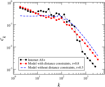
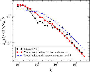
Figure 3: Clustering coefficient, $c_{k}$ (top) and normalised average nearest neighbors degree, $\bar{k}_{nn}(k)\langle k\rangle/\langle k^{2}\rangle$ (bottom), as functions of the node’s degree for the extended autonomous system map (circles) and for the model with and without distance constraints (red squares and dashed line, respectively).

Fig. 2 shows simulation results for the cumulative degree distribution, in nice agreement to that measured for the AS+ map. The inset exhibits simulation results of the AS’s degree as a function of the AS’s bandwidth, conforming to the scaling relation in Eq. (11). Clustering coefficient and average nearest neighbors degree are showed in Fig. 3. Dashed lines result from the model without distance constraints, whereas squares correspond to the model with distance constraints. Interestingly, the high level of clustering coming out from the model arises as a consequence of the pattern followed to attach nodes, so that only those AS willing for new connections will link. As can be observed in the figures, distance constraints introduce a disassortative component by inhibiting connections between small ASs so that the hierarchical structure of the real network is better reproduced.

We conclude by pointing out that this work is a first attempt towards a more realistic and complete modeling of the Internet, which, for instance, is of utmost importance in new communication protocols testing, which can be very sensitive to topological details. We would like to stress that the relevance of our model resides in the robustness of a simple statistical physics approach and, as a result, the unprecedented completedness of the topological description of the Internet and the novel insights into the dynamical processes leading to network formation.