Self-organization of structures and networks from merging and small-scale fluctuations.

Abstract

We discuss merging-and-creation as a self-organizing process for scale-free topologies in networks. Three power-law classes characterized by the power-law exponents 3/2, 2 and 5/2 are identified and the process is generalized to networks. In the network context the merging can be viewed as a consequence of optimization related to more efficient signaling.

1 Introduction

Natural processes often lead to spatially non-uniform distributions of physical quantities. In particular scale-free structures are intriguing because they suggest dynamic principles that are universally applicable [1, 2, 3, 4]. Recently it has been realized that many complex networks exhibit scale-free topologies [5, 6, 7]. In general, the first theoretical framework for such very skew distributions was the Simon model [8], featuring a “rich get richer” process, that recently has been developed into preferential attachment to explain scale-free networks [6]. Another approach to such broad distributions is the Self Organized Critical models that were put forward by Per Bak and coworkers [2, 3, 4] and were suggested for networks by [9, 10]. In these models large-scale structures and intermittent activity emerge as a consequence of small-scale excitations of systems with inherent memory. In the present paper we elaborate on another class of Self-Organization models, based on the ”Aggregation with Injection” scenario [11, 12, 13, 14, 15, 16]. Interpreted as a merging-and-creation process, reviewing [17, 18], we apply this class to complex networks and show that scale-free topologies emerge. The merging-and-creation process spontaneously generates power-law distributions by a mechanism which is quite different from the “rich get richer” scenario. As in the SOC models it is based on a non-equilibrium bottom up scenario, where a scale-free distribution of structures is obtained at steady state. Thus it indeed is an appealing alternative to the preferential attachment models that has been suggested for growing networks.

2 The merging-and-creation process

The basic “merging-and-creation” process can be described in terms of the evolution of a system of many elements $i=1,2,....,N$, each characterized by a scalar $q_{i}$. The scalar may be either just positive [11] or both positive and negative [14, 16].

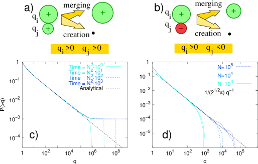
Figure 1: a) and b) illustrate the basic merging-and-creation process with b) associated to merging of elements with different signs. c) Refers to a merging of only positive elements, with creation due to injection from outside. The figure shows the cumulative distribution $P(>q)=\sum_{m=q}^{\infty}P(m)$ at different times from the start averaged over $M=1000$-realizations for a system with $N=10^{3}$ elements. The dashed curve is the exact solution that scales as $P(>q)\propto q^{1-\gamma}$ with $\gamma=3/2$ for large $q$. The numerical simulations are for three different times and agree with the scaling up to some cutoff. The deviation from the power-law above the cutoff reflects that, in addition, there is a single growing, large element, $q\propto time$ with $P(q)=1/N$. The total sum $Q=\sum^{\prime}q_{i}$ of all the other $q^{\prime}s$ approaches a constant steady state value. d) Refers to symmetric process where both positive and negative elements can be merged (as the combined a) and b)). The steady state distribution $P(>q)$, obtained numerically, is shown for three sizes $N$. The exact asymptotic solution is given by the dashed line ($\propto q^{-1}$).

As a concrete example one may think of the elements as particles and the scalar as the mass of a particle. Other examples are nodes of a network and the number of links attached to a node; companies and the financial assets of the company; vortices and the vorticity of a vortex and so forth.

The prototype of the process describes a situation in which the elements in the system redistribute their corresponding $q_{i}$ according to a merging step where two elements $i$ and $j$ are chosen (typically randomly) and then are merged together. For illustration see Fig. 1ab. The merged element acquires the sum of the scalars $q_{i}+q_{j}$. We express this as

$$merging:\;\;\;q_{i} \rightarrow q_{i}+q_{j}$$

$$q_{j} \rightarrow 0,$$ (1)

where the second process means that the element $i$ is replaced by an empty element. This ensures that the number of elements remain constant. In parallel to this, there is a creation process of elements with small $|q|\neq 0$. This corresponds to adding a scalar $q=\pm 1$ to an empty element:

$$creation:\;\;\;q_{k}=0 \rightarrow q_{k}=\pm 1.$$ (2)

We either ensure that the average $q$ of the system does not change by choosing $+1$ or $-1$ with equal probability in the creation step (see Fig. 1ab) or we consider the case when the average $q$ is growing by choosing $+1$ every time (see Fig. 1a). Obviously there is a multitude of variants to this process, including for example the case where the creation event is also allowed on $q\neq 0$ elements. These variations of the merging-and-creation processes can be classified into three categories, each characterized by a unique power-law exponent for the distribution of scalars $q$ among the elements.

• Category $\gamma=3/2$
  The prototype process [11, 12, 13] can be described as

  $$merging:\;\;\;q_{i} \rightarrow q_{i}+q_{j}$$

  $$q_{j} \rightarrow 0$$

  $$creation:\;\;\;q_{k}=0 \rightarrow q_{k}=1.$$ (3)

  Here we imagine that we have a large number of elements $N$ and start the process from all $q_{i}=0$. At each step the average scalar $\langle q\rangle$ is increased by $1/N$. Fig. 1a illustrates the basic process and Fig. 1c shows the result from simulations using this initial condition (averaged over many realizations). As seen the probability distribution that an element has a value $q$, $P(q)$, is a power-law with a slope that to good approximation is given by $\gamma=3/2$ i.e. $P(q)\propto q^{-3/2}$ apart from a single growing large $q$-element. Thus the growth of the average only results in the growth of a single largest element. The rest of the distribution is stationary and furthermore this stationary solution is independent of the starting condition.

  In terms of the probability distribution $P$ the condition for a stationary solution in the limit of large $N$ is given by

  $$\sum_{q_{1},q_{2}}P(q_{1})P(q_{2})\delta_{q_{1}+q_{2},q}-2P(q)+\delta_{q,1}=0,$$ (4)

  which for $q=0$ gives $P(0)=0$ and provides a recursive solution for subsequent $q$’s. As a result [11, 12, 13] one obtains a steady state distribution with asymptotic behavior $P(q)\propto q^{-3/2}$.

• Category $\gamma=2$
  This corresponds to the symmetric case were $P(q)=P(-q)$. The prototype for this process [14, 16] is the same as for the previous case except for a symmetric creation: $q_{k}=0\rightarrow q_{k}=\pm 1$ (see Fig. 1b). This means that the average $\langle q\rangle$ now is unchanged during the process. Again we start with $N$ empty elements ($q_{i}=0,\forall i$). Fig. 1d shows the result from simulations. A power-law distribution with $\gamma=2$ is generated to good approximation.

  The steady state solution in terms of $P(q)$ is this time given by

  $$\sum_{q_{1}q_{2}}P(q_{1})P(q_{2})\delta_{q_{1}+q_{2},q}-2P(q)+\frac{1}{2}[\delta_{q,1}+\delta_{q,-1}]=0.$$ (5)

  which has the asymptotic solution $P(q)\propto 1/q^{2}$ as demonstrated by Takaysu in Ref.[14]. In addition, the robustness of this scaling behavior is remarkable: If one instead of starting from a symmetric distribution with average $\langle q\rangle=0$, starts from a situation with an excess average $\langle q\rangle\neq 0$ then all the excess ($\langle q\rangle N$) will be collected on a single large element [18]. This is similar to what was found for the growing case with $\gamma=1.5$.

• Category $\gamma=5/2$
  Here we consider the process of merging and spontaneous fluctuations among positive elements. Thus no negative elements are allowed, but in contrast to the $\gamma=3/2$ case the average $\langle q\rangle$ is not growing. This is achieved if at every merging step there is some small loss, i.e.

  $$q_{i}\rightarrow q_{i}+q_{j}-1\;\;\;\mbox{and}\;\;\;\;q_{j}\rightarrow r,$$

  where $r\in[0,2]$ is a random number from a narrow distribution $\langle r\rangle=1$ and $q$ is constrained to be $\geq 0$. The process in general corresponds to merging of positive elements, but also allows for spontaneous ”evaporation” (when one $q$-value is zero). This process is in fact also equivalent to a number of other conserving processes ($q_{i}\rightarrow q_{i}+q_{j}-r$ and $q_{j}\rightarrow r$) subject to the size constraint that all $q$ should be larger than some $q_{c}$.

  It deals with situations where also the largest element can sometimes lose in the merging step, under the constraint of a lowest allowed value of $q$.

  With the transformation $q\rightarrow q-1$ the model is equivalent to the process

  $$q_{i}=q_{i}+q_{j},\;\;\;\mbox{and}\;\;q_{j}=\pm 1$$ (6)

  This is mathematically equivalent to the symmetric process with $\gamma=2$ with the additional constraint that no element can have a scalar less than $q=-1$. Any random choice of two elements which would lead to a merged element violating the constraint is abandoned and a new random choice is made. One notices that because the creation is symmetric with respect to $q_{c}=\pm 1$ the average value $\langle q\rangle$ is preserved ($\langle q\rangle=0$ when starting from a symmetric distribution). Fig. 2a gives the result from a numerical simulation. The data falls on the straight line corresponding to a power-law distribution with $\gamma=2.5$.

  

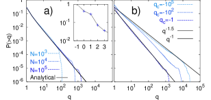
  Figure 2: a) The steady-state distribution $P(>q)=\sum_{m=q}^{\infty}P(m)$ obtained from simulations for three sizes $N$ for the case with constrained $q$ values (case $\gamma=5/2$). The exact asymptotic form is given by the full curve ($\propto q^{-3/2}$). The inset gives the comparison between the exact solution and the simulations for the smallest $q$-values. b) The steady state distribution $P(>q)$ for three different constraints $q_{c}=-1,-100$, and $-N$, respectively. Here the system size is $N=10^{5}$. Power-laws with $\gamma=2.5$ and $\gamma=2$ correspond to the slopes of the full lines. The figure illustrates the cross-over from the case $\gamma=2.5$ to the case $\gamma=2$ as the constraint on possible $q$ values is relaxed.

  The steady state solution in terms of $P(q)$ is obtained is obtained in the same way as in the previous cases but the constraint changes the steady state condition into

  $$\sum_{-1}^{\infty}\frac{P(q_{1})P(q_{2})}{1-P(-1)^{2}}\delta_{q_{1}+q_{2},q}\; - \;\frac{2P(q)}{1-P(-1)^{2}}+$$

  $$+\frac{2P(-1)^{2}\delta_{q,-1}}{1-P(-1)^{2}}\; + \;\frac{\left[\delta_{q,-1}+\delta_{q,1}\right]}{2}\;=\;0.$$ (7)

  This equation has a simple recursive solution since the $q=-1$ and 0 cases directly give

  $$P(0)=1-\frac{3}{4}P(-1)-\frac{1}{4P(-1)}\;\;\;\mbox{and}\;\;\;P(1)=\frac{P(0)}{P(-1)}-\frac{P(0)^{2}}{2P(-1)}$$

  Eq. (• ‣ 2) leads to an equation in terms of $g(\alpha)=\sum_{0}^{\infty}P(q)e^{-\alpha q}$ given by

  $$g(\alpha)^{2}-2g(\alpha)-P(-1)^{2}(e^{2\alpha}-2e^{\alpha})+(1-P(-1)^{2})\cosh(\alpha)=0,$$

  which has the solution

  $$g(\alpha)=1-\sqrt{1+P(-1)^{2}(e^{2\alpha}-2e^{\alpha})-(1-P(-1)^{2})\cosh(\alpha)}.$$ (8)

  Expanding the argument of the square root in $\alpha$ gives

  $$(3P(-1)^{2}/2-1/2)\alpha^{2}+P(-1)^{2}\alpha^{3}.$$

  Now the zero order moment is just $g(0)=\int dqP(q)=1$ as it must. The second order moment must vanish by the condition $\langle q\rangle=0$: If $3P(-1)^{2}/2-1/2$ is negative then there is no solution and if it is positive then the first moment $\langle q\rangle\neq 0$. So the only possibility is $P(-1)=\sqrt{1/3}$ which also means that the leading $\alpha$-dependence of the square root in Eq. (8) is proportional to $\alpha^{3/2}$. This in turn means that in this case the second moment diverges as

  $$\sum^{1/\alpha}P(q)q^{2}\sim\frac{1}{\sqrt{\alpha}}$$

  and it follows that the leading behavior of $\gamma$ is given by $\gamma-3=-1/2$ or $\gamma=5/2$.

  The exact solution can be obtained from the recursive relation starting with $P(-1)=\sqrt{1/3}$ and is plotted in Fig. 2a and its inset. Fig. 2b shows the cross-over from the case with $\gamma=2.5$ to the completely symmetric case with $\gamma=2$, by successively relaxing the constraint from $q\geq-1$ to $q\geq-N$.

3 Network version

Let us now discuss the merging-and-creation process in the context of evolving networks. The motivation for such a process in these types of complex systems is the gain in “simplification” that one obtains by merging nodes, supplemented by an overall drive to invent or excite the system by new nodes with new connections. The merging-and-creation scenario for networks were presented in Ref. [17, 18], where it was shown numerically that also for networks the merging-and-creation gives rise to power-law distributions in parallel with the scalar version discussed in the present version. A simple network version goes as follows:

• Choose two nodes $i$ and $j$ randomly. The corresponding scalar is the degree of the node (the number of links attached to a node).

• The nodes $i$ and $j$ are merged together to a node $m$ of degree $k_{m}=k_{i}+k_{j}-N_{common}$ results, with $N_{common}$ being the number of nodes that are neighbors to both $i$ and $j$. These common links are deleted from the network (if $i$ and $j$ are joined by a link this is also counted as a common link). Thereby multiple links between pairs of nodes are removed.

• A new node of degree $k_{new}$ is added to the network with the links attached to $k_{new}$ random nodes. The degree $k_{new}$ of the added node is a random number picked from a uniform distribution centered around some number $\langle r\rangle$.

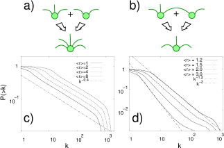
Figure 3: a) Illustrates the merging move of the two random nodes and b) illustrates the merging of neighbors. c) Simulation of the network version of the merging-and-creation process for $N=2^{14}$ and $\langle r\rangle=2,4$ and $8$. The cumulative degree distribution $P(>k)$ for the network version is shown to have a power-law distribution $P(>k)\propto k^{(1-\gamma)}$ with $\gamma\rightarrow 3/2$ for $N\rightarrow\infty$. d) Simulation of the network version with the constraint of merging only of neighbors for $N=2^{14}$. In this case the power-law exponent is a function of $\langle r\rangle$ and varies from $\gamma=2$ to $\gamma=3$.

Fig. 3a shows that this network version of merging-and-creation gives rise to a power-law distribution with $\gamma=3/2$ ( for any $\langle r\rangle\geq 1$) as expected for this process applied to positive quantities.

However, a real network implementation of merging-and-creation would rather consists of local topological rearrangements which facilitate performance. Thus we consider the case where one node is constrained to be the random neighbor of the other in the merging process [17]. This would be reasonable in molecular networks where one protein takes over the regulatory functions of a neighboring protein in order to shorten the signaling pathways. With this simple constraint on the merging-and-creation process the power-law exponent $\gamma$ becomes a function of $\langle r\rangle$ as demonstrated in Fig. 3b, where $\gamma$ varies from $3$ to $2$ with increasing $\langle r\rangle$.

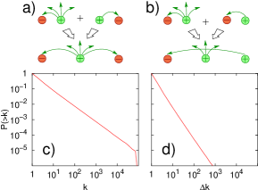
Figure 4: The network realization of the symmetric model. a) and b) illustrate possible merging moves. Positive vertices (donors) are vertices with outgoing edges and negative (acceptors) with incoming edges. c) The cumulative probability distributions, $N=10^{5}$, for number of edges incoming or outgoing from a node. The distribution is scale-free $P(>\!\!k)\sim 1/k^{\gamma-1}$ with $\gamma=2$. d) The cumulative probability distributions for the changes in number of edges due to merging, $\Delta k$. The distribution is power-law $P(>\!\!\Delta k)\sim{\Delta k}^{1-\tau}$ with exponent $\tau=2\gamma-1=3$ from Eq. 4.

Another interesting network application is related to merging of sun spots and associated magnetic field lines in the solar atmosphere [9, 18]. In this case there are sun-spots of two polarities, and the network consists of magnetic field lines that make directed connections between the sun spots. In this case the sign (polarity) would correspond to the number of in- or out-edges [18]. Each vertex may have different number of edges, but at any time a given vertex cannot be both donor and acceptor. Further, in the direct generalization of the symmetric $\gamma=2$ case, we allow several parallel edges between any pair of vertices. At each time-step two vertices $i$ and $j$ are chosen randomly. The basic update is shown in panel a), b) of Fig. 4, and the result in terms of number of edges from any node counting multiple edges is shown in Fig. 4c. Also interesting in this case is the activity of events of sun spot assimilations, exhibiting a scaling $1/q^{3}$ also found in the more detailed model of cascading magnetic loops in solar atmosphere by Hughes and Paczuski [9, 10].

In summary, merging-and-creation opens for a new way of viewing spontaneous emergence of scale-free networks, associated to systems where there is an ongoing tendency of simplification by merging.

References

- [1] T. A. Witten Jr, L. M. Sander, Phys. Rev. Lett. 47, 1400 (1981).
- [2] P. Bak, C. Tang and K. Wiesenfeld, Phys. Rev. Lett. 59, 381-374 (1987).
- [3] P. Bak, K. Chen, C. Thang, Phys. Lett. 147, 297 (1990).
- [4] P. Bak and K. Sneppen, Phys. Rev. Lett. 71, 4083 (1993).
- [5] M. Faloutsos, P. Faloutsos, and C. Faloutsos, Comput. Commun. Rev. 29, 251 (1999).
- [6] A.-L. Barabási, R. Albert, Science, 286, 509 (1999).
- [7] A. Broder et al. S. Rajagopalan, R. Stata, A. Tomkins, J. Wiener, Computer Networks 33, 309 (2000).
- [8] H. Simon, Biometrika 42, 425 (1955).
- [9] D. Hughes, M. Paczuski, R.O. Dendy, P. Helander and K.G. McClements. Physical Rev. Letters 90, 131101 (2003).
- [10] M. Paczuski and D. Hughes, cond-mat/0311304 (2003).
- [11] G.B. Field and W.C. Saslow, Astrophys. J. 142, 568 (1965)
- [12] H. Hayakawa and S. Hayakawa Publ. Astron. Soc. Japan 40, 341-345 (1988).
- [13] H. Hayakawa J. Phys. A., 20, L801 (1987).
- [14] H. Takayasu, Phys. Rev. Lett. 63 2563, (1989)
- [15] H. Takayasu, M. Takayasu, A. Provata and G. Huber, J. Stat. Phys. 65, 725 (1991).
- [16] P.L. Krapivsky, Physica A 198, 157 (1993).
- [17] B.J. Kim, A. Trusina, P. Minnhagen, and K. Sneppen, preprint NORDITA-2004-9 (2004).
- [18] K.Sneppen, M. Rosvall, A. Trusina, and P. Minnhagen, preprint NORDITA-2004-10 (2004).