Unusual localisation effects in quantum percolation

Abstract

We present a detailed study of the quantum site percolation problem on simple cubic lattices, thereby focussing on the statistics of the local density of states and the spatial structure of the single particle wavefunctions. Using the Kernel Polynomial Method we refine previous studies of the metal-insulator transition and demonstrate the non-monotonic energy dependence of the quantum percolation threshold. Remarkably, the data indicates a “fragmentation” of the spectrum into extended and localised states. In addition, the observation of a chequerboard-like structure of the wavefunctions at the band centre can be interpreted as anomalous localisation.

Disordered structures attracted continuing interest over the last decades, and besides the Anderson localisation problemAnderson (1958) quantum percolationKirkpatrick and Eggarter (1972); Mookerjee et al. (1995) is one of the classical subjects of this field. Current applications concern e.g. transport properties of doped semiconductorsInui et al. (1994) and granular metalsFeigel’mann et al. (2004), metal-insulator transition in two-dimensional n-GaAs heterostructuresDas Sarma et al. (2004), wave propagation through binary inhomogeneous mediaAvishai and Luch (1992), superconductor-insulator and (integer) quantum Hall transitionsDubi et al. (2004); Sandler et al. (2003), or the dynamics of atomic Fermi-Bose mixturesSanpera et al. (2004). Another important example is the metal-insulator transition in perovskite manganite films and the related colossal magnetoresistance effect, which in the meantime are believed to be inherently percolative.Becker et al. (2002)

In disordered solids the percolation problem is characterised by the interplay of pure classical and quantum effects. Besides the question of finding a percolating path of “accessible” sites through a given lattice the quantum nature of the electrons imposes further restrictions on the existence of extended states and, consequently, of a finite DC-conductivity. As a particularly simple model describing this situation we consider a tight-binding one-electron Hamiltonian,

$${H}=\sum_{i=1}^{N}\epsilon_{i}{c}_{i}^{{\dagger}}{c}_{i}-t\sum_{\langle ij\rangle}({c}_{i}^{{\dagger}}{c}_{j}+\text{H.c.})\,,$$ (1)

on a simple cubic lattice with $N=L^{3}$ sites and random on-site energies $\epsilon_{i}$ drawn from the bimodal distribution

$$p(\epsilon_{i})=p\,\delta(\epsilon_{i}-\epsilon_{A})+(1-p)\,\delta(\epsilon_{i}-\epsilon_{B})\,.$$ (2)

The two energies $\epsilon_{A}$ and $\epsilon_{B}$ could, for instance, represent the potential landscape of a binary alloy A_pB_1-p, where each site is occupied by an A or B atom with probability $p$ or $1-p$, respectively. In the limit $\Delta=(\epsilon_{B}-\epsilon_{A})\rightarrow\infty$ the wavefunction of the $A$ sub-band vanishes identically on the $B$-sites, making them completely inaccessible for the quantum particles. We then arrive at a situation where non-interacting electrons move on a random ensemble of lattice points, which, depending on $p$, may span the entire lattice or not. The corresponding Hamiltonian reads

$${H}=-t\!\sum_{\langle ij\rangle\in A}\!({c}_{i}^{{\dagger}}{c}_{j}+\text{H.c.})\,,$$ (3)

where the summation extends over nearest-neighbour $A$-sites only and, without loss of generality, $\epsilon_{A}$ is chosen to be zero.

Within the classical percolation scenario the percolation threshold $p_{c}$ is defined by the occurrence of an infinite cluster $A_{\infty}$ of adjacent $A$ sites. For the simple cubic lattice this site-percolation threshold is $p_{c}=0.3117$.Heermann and Stauffer (1981) In the quantum case, the multiple scattering of the particles at the irregular boundaries of the cluster can suppress the wavefunction, in particular, within narrow channels or close to dead ends of the cluster. Hence, this type of disorder can lead to absence of diffusion due to localisation, even if there is a classical percolating path through the crystal. On the other hand, for finite $\Delta$ the tunnelling between $A$ and $B$ sites may cause a finite DC-conductivity although the $A$ sites are not percolating. Naturally, the question arises whether the quantum percolation threshold $p_{q}$, given by the probability above which an extended wavefunction exists within the $A$ sub-band, is larger or smaller than $p_{c}$. Previous results Soukoulis et al. (1992) for finite values of $\Delta$ indicate that the tunnelling effect has a marginal influence on the percolation threshold as soon as $\Delta\gg 4tD$, where $D$ denotes the spatial dimension of the hypercubic lattice.

In the theoretical investigation of disordered systems it turned out that distribution functions for the random quantities take the centre stage.Anderson (1958); Abou-Chacra et al. (1973) The distribution $f(\rho_{i}(E))$ of the local density of states (LDOS),

$$\rho_{i}(E)=\sum\limits_{n=1}^{N}|\psi_{n}({\bf r}_{i})|^{2}\,\delta(E-E_{n})\,,$$ (4)

is particularly suited because $\rho_{i}(E)$ measures the local amplitude of the wavefunction at site ${\bf r}_{i}$. It therefore contains direct information about the localisation properties. In contrast to the (arithmetically averaged) mean DOS, $\rho_{\rm me}(E)=\langle\rho_{i}(E)\rangle$, the LDOS becomes critical at the localisation transition.Haydock and Te (1994); Dobrosavljević et al. (2003) The probability density $f(\rho_{i}(E))$ was found to have essentially different properties for extended and localised phases.Mirlin and Fyodorov (1994) For an extended state at energy $E$ the amplitude of the wavefunctions is more or less uniform. Accordingly $f(\rho_{i}(E))$ is sharply peaked and symmetric about $\rho_{\rm me}(E)$. On the other hand, if states become localised, the wavefunction has considerable weight only on a few sites. In this case the LDOS strongly fluctuates throughout the lattice and the corresponding LDOS distribution is very asymmetric and has a long tail. Above the localisation transition the distribution of the LDOS is singular, i.e., mainly concentrated at $\rho_{i}=0$. Nevertheless the rare but large LDOS-values dominate the mean DOS $\rho_{\rm me}(E)$, which therefore cannot be taken as a good approximation of the most probable value of the LDOS. Such systems are referred to as “non-self-averaging”. Of course, for practical calculations the recording of entire distributions is a bit inconvenient. Instead the mean DOS $\rho_{\rm me}(E)$ together with the (geometrically averaged) so-called “typical” DOS, $\rho_{\rm ty}(E)=\exp\langle\ln\rho_{i}(E)\rangle$, is frequently used to monitor the transition from extended to localised states. The typical DOS puts sufficient weight on small values of $\rho_{i}$ and a comparison to $\rho_{\rm me}(E)$ therefore allows to detect the localisation transition. This has been shown for the pure Anderson modelDobrosavljević et al. (2003); Schubert et al. (2003); Alvermann et al. (2004) and for even more complex situations, where the effects of correlated disorderSchubert et al. (2004), electron-electron interactionDobrosavljević and Kotliar (1997); Byczuk et al. (2004) or electron-phonon couplingBronold and Fehske (2002); Bronold et al. (2004) were taken into account.

In this paper we employ the typical-DOS concept to analyse the nature of the eigenstates (extended or localised) of the Hamiltonians (1) and (3). Using the Kernel Polynomial MethodSilver et al. (1996); Schubert et al. (2003), an efficient high-resolution Chebyshev expansion technique, in a first step, we calculate the LDOS for a large number of samples, $K_{r}$, and sites, $K_{s}$. The mean DOS is then simply given by

$$\rho_{\text{me}}(E)=\frac{1}{K_{r}K_{s}}\smash{\sum\limits_{k=1}^{K_{r}}\sum\limits_{i=1}^{K_{s}}\rho_{i}(E)}\,,$$ (5)

whereas the typical DOS is obtained from the geometric average

$$\rho_{\text{ty}}(E)=\exp\left(\frac{1}{K_{r}K_{s}}\smash{\sum\limits_{k=1}^{K_{r}}\sum\limits_{i=1}^{K_{s}}\ln\bigl{(}\rho_{i}(E)\bigr{)}}\right)\,.$$ (6)

We classify a state at energy $E$ with $\rho_{\rm me}(E)\neq 0$ as localised if $\rho_{\rm ty}(E)=0$ and as extended if $\rho_{\rm ty}(E)\neq 0$.

Before discussing possible localisation phenomena let us investigate the behaviour of the mean DOS for the quantum percolation models (1) and (3). Figure 1 shows that as long as $\epsilon_{A}$ and $\epsilon_{B}$ do not differ too much there exists an asymmetric (if $p\neq 0.5$) but still connected electronic band.Soukoulis et al. (1992) At about $\Delta\simeq 4tD$ this band separates into two sub-bands centred at $\epsilon_{A}$ and $\epsilon_{B}$, respectively. The most prominent feature in the split-band regime is the series of spikes at discrete energies within the band. As an obvious guess, we might attribute these spikes to eigenstates on islands of $A$ or $B$ sites being isolated from the main cluster.Kirkpatrick and Eggarter (1972); Berkovits and Avishai (1996) It turns out, however, that some of the spikes persist, even if we neglect all finite clusters and restrict the calculation to the spanning cluster of $A$ sites, $A_{\infty}$. This is illustrated in the upper panels of Fig. 2, where we compare the DOS of the models (1) [at $\Delta\to\infty$] and (3). Increasing the concentration of accessible sites the mean DOS of the spanning cluster is evocative of the DOS of the simple cubic lattice, but even at large values of $p$ a sharp peak structure remains at $E=0$ (cf. Fig. 2, lower panels).

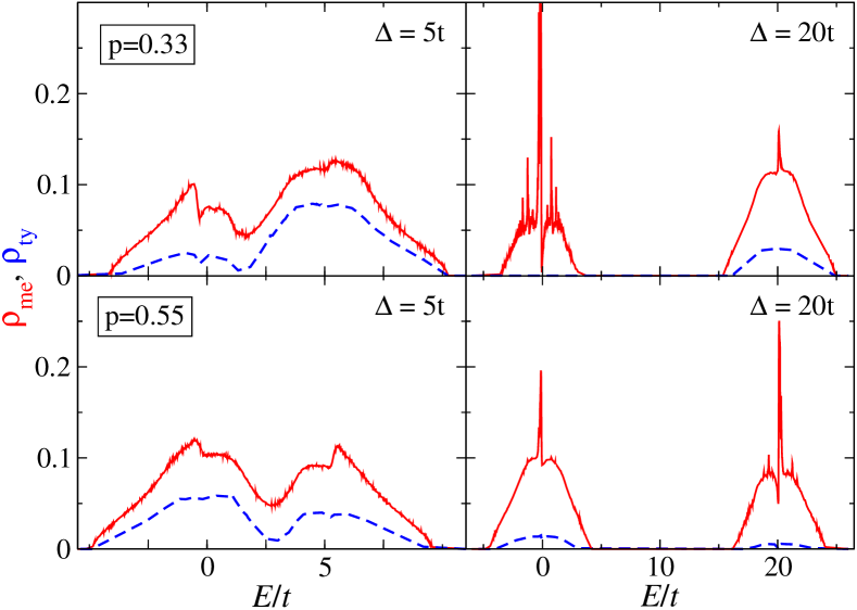
Figure 1: (Colour online) Mean (solid line) and typical (dashed line) DOS of the Hamiltonian (1) on a $50^{3}$ lattice with periodic boundary conditions (PBC). Results are obtained using $M=32768$ Chebyshev moments and $K_{s}\times K_{r}=32\times 32$ realisations.

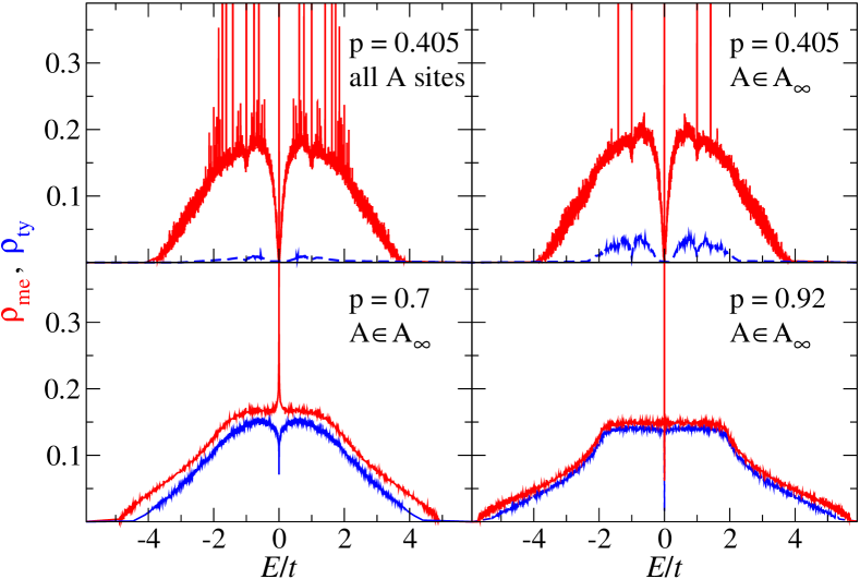
Figure 2: (Colour online) Mean (solid line) and typical (dashed line) DOS for the quantum percolation model in the limit $\Delta\to\infty$. While in the upper left panel all $A$-sites are taken into account, the other three panels show data for the restricted model (3) on the spanning cluster $A_{\infty}$ only (note that $\rho_{\rm ty}$ is smaller in the former case because there are more sites with vanishing amplitude of the wavefunction). System sizes were adapted to ensure that $A_{\infty}$ always contains the same number of sites, i.e., $N=57^{3}$ for $p=0.405$, $46^{3}$ for $p=0.70$, and $42^{3}$ for $p=0.92$. Again we used $M=32768$ and $K_{s}\times K_{r}=32\times 32$.

To elucidate this effect, which partially is not accounted for in the literatureKirkpatrick and Eggarter (1972); Odagaki et al. (1980); Soukoulis et al. (1987, 1992), in more detail, in Fig. 3 we fixed $p$ at $0.33$, shortly above the classical percolation threshold, and increased the ensemble size. Besides the most dominant peaks at $E/t=0,\pm 1,\pm\sqrt{2}$, in addition we can resolve distinct spikes at $E/t=\frac{1}{2}\left(\pm 1\pm\sqrt{5}\right),\pm\sqrt{3},\pm\sqrt{2\pm\sqrt{2}},\ldots$ These special energies coincide with the eigenvalues of the tight-binding model on small clusters of the geometries shown in the right part of Fig. 3. In accordance with Refs. Kirkpatrick and Eggarter, 1972 and Chayes et al., 1986 we can thus argue that the wavefunctions, which correspond to these special energies, are localised on some “dead ends” of the spanning cluster.

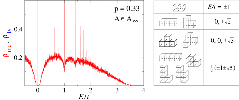
Figure 3: (Colour online) Left: Mean (solid line) and typical (dashed line) DOS for the model (3) with $p=0.33$ on a $100^{3}$ lattice (PBC, $M=32768$). Data obtained from an average over $100$ random initialisations of sites for $K_{r}=100$ realisations of disorder. Note that $\rho_{ty}<10^{-5}$ holds in the whole band. Right: Some cluster configurations related to the special energies at which the peaks in $\rho_{\text{me}}$ occur.

The assumption that the distinct peaks correspond to localised wavefunctions is corroborated by the fact that the typical DOS vanishes or, at least, shows a dip at these energies. Occurring also for finite $\Delta$ (Fig. 1), this effect becomes more pronounced as $\Delta\to\infty$ and in the vicinity of the classical percolation threshold $p_{c}$. From the study of the Anderson model Anderson (1958) we know that localisation leads at first to a narrowing of the energy window containing extended states. The corresponding mobility edges have been mapped out with high precision.Mac Kinnon and Kramer (1983); Alvermann et al. (2004) For the percolation problem, in contrast, with decreasing $p$ the typical DOS indicates both localisation from the band edges and localisation at particular energies within the band. Since finite cluster wavefunctions like those shown in Fig. 3 can be constructed for numerous other, less probable geometries Schubert (2003), Chayes et al. (1986) argued that an infinite discrete series of such spikes might exist within the spectrum. The picture of localisation in the quantum percolation model is then quite remarkable. If we generalise our numerical data for the peaks at $E=0$ and $E/t=\pm 1$, it seems as if there is an infinite discrete set of energies with localised wavefunctions, which is dense within the entire spectrum. In between there are continua of delocalised states, but to avoid mixing, their density goes to zero close to the localised states. Facilitated by the large special weight of the peak (up to 10% close to $p_{c}$) this is clearly observed at $E=0$, and we suspect similar behaviour at $E/t=\pm 1$. For the other discrete spikes the resolution of our numerical data is still too poor and the system size might be even too small to draw a definite conclusion.

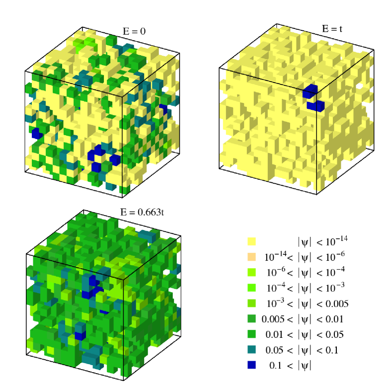
Figure 4: (Colour online) Amplitudes of the wavefunction, $|\psi_{n}({\bf r}_{i})|$, of the quantum percolation model (3) on $A_{\infty}$ of a $14^{3}$ lattice with occupation probability $p=0.45$. Exact diagonalisation results are presented at three characteristic energies $E/t=0$, 1, and 0.66 corresponding to anomalously localised, localised, and delocalised states, respectively.

In order to understand the internal structure of the extended and localised states we calculated the amplitudes of the wavefunction at specific energies for a random sample of the quantum percolation model (3) restricted to $A_{\infty}$. Figure 4 visualises the spatial variation of $|\psi_{n}({\bf r_{i}})|$ on a $14^{3}$ lattice with PBC and an occupation probability $p=0.45$ well above the classical percolation threshold. The figure clearly indicates that the state with $E/t=0.66$ is extended, i.e. the spanning cluster is quantum mechanically “transparent”. On the contrary, at $E=t$, the wavefunction is completely localised on a finite region of the spanning cluster. Here the scattering of the particle at the random surface of the spanning cluster results in states, where the wavefunction vanishes identically except for some finite domains on loose ends (like those shown in Fig. 3), where it takes the values ($\pm 1,\mp 1$), ($\pm 1,\mp 1,0,\mp 1,\pm 1$), $\ldots$ Note that these regions are part of the spanning cluster, connected to the other sites by a site with wavefunction amplitude zero. A particularly interesting behaviour is observed at $E=0$. The eigenstate $E=0$ is highly degenerate and we can form wavefunctions that span the entire lattice in a chequerboard structure with zero and non-zero amplitudes (see Fig. 4). Although these states are extended in the sense that they are not confined to some region of the cluster, they are localised in the sense that they do not contribute to the DC-conductivity. This is caused by the alternating structure which suppresses the nearest-neighbour hopping, and in spite of the high degeneracy, the current matrix element between different $E=0$ states is zero. Hence, having properties of both classes of states these states are called anomalously localised.Shapir et al. (1982); Inui et al. (1994) The chequerboard structure is also observed for the hypercubic lattice in 2D but with reduced spectral weight, compared to the 3D case. Another indication for the robustness of this feature is its persistence for mismatching boundary conditions, e.g., periodic (antiperiodic) boundary conditions for odd (even) values of the linear extension $L$. In these cases the chequerboard is matched to itself by a manifold of sites with vanishing amplitude.

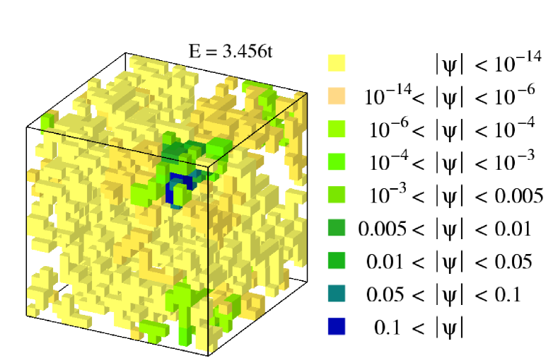
Figure 5: (Colour online) Amplitudes $|\psi_{n}({\bf r}_{i})|$ of a localised state on a $21^{3}$ lattice with $p=0.33$ obtained by exact diagonalisation of the model (3). $E/t=3.456$ was chosen in order to avoid any of the special cluster configurations discussed above.

In the past most of the methods used in numerical studies of Anderson localisation have also been applied to the percolation models (1) or (3) in order to determine the quantum percolation threshold $p_{q}$, defined as the probability $p$ below which all states are localised (see, e.g., Refs. Mookerjee et al., 1995; Koslowski and von Niessen, 1990 and references therein). However, so far the results for $p_{q}$ are far less precise than, e.g., the values of the critical disorder reported for the Anderson model. For the simple cubic lattice numerical estimates of quantum site-percolation thresholds range from 0.4 to 0.5. In Figs. 1-3 we presented data for $\rho_{\rm ty}$ which shows that $p_{q}>p_{c}$. In fact, within numerical accuracy, we found $\rho_{\rm ty}=0$ for $p=0.33>p_{c}$. Figure 5 displays the amplitude of a typical state obtained by exact diagonalisation for a fixed realisation of disorder. Bearing in mind that we have used PBC, the support of the wavefunction appears to be a finite (connected) region of the spanning cluster $A_{\infty}$, i.e., the state is clearly localised.

To get a more detailed picture we calculated the normalised typical DOS, $R(p,E)=\rho_{\rm ty}/\rho_{\rm me}$, in the whole concentration-energy plane. Figure 6 presents such kind of phase diagram of the quantum percolation model (3). The data supports a finite quantum percolation threshold $p_{q}\gtrsim 0.4>p_{c}$ (cf. also Refs. Koslowski and von Niessen, 1990; Soukoulis et al., 1992; Kusy et al., 1997; Kaneko and Ohtsuki, 1999), but as the discussion above indicated, for $E=0$ and $E=\pm t$ the critical value $p_{q}(E)$ is $1$, and the same may hold for the set of other “special” energies. The transition line between localised and delocalised states, $p_{q}(E)$, might thus be a rather irregular (fractal?) function. On the basis of our numerical treatment, however, we are not in the position to answer this question with full rigour.

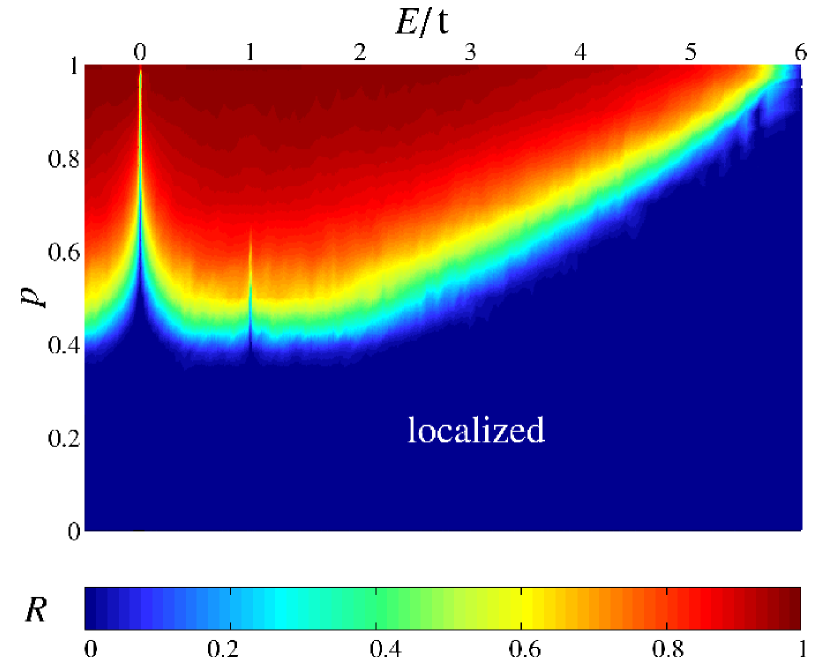
Figure 6: (Colour online) Normalised typical DOS $R=\rho_{\rm ty}/\rho_{\rm me}$ in the concentration-energy plane for the model (3) on a $50^{3}$ lattice for $p\geq 0.5$ and a $100^{3}$ lattice for $p<0.5$. We used $M=16384$ Chebyshev moments and averaged over $K_{s}\times K_{r}=32\times 32$ realisations.

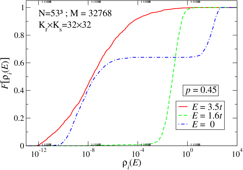
Figure 7: (Colour online) Characteristic probability distributions of the LDOS.

Finally let us come back to the characterisation of extended and localised states in terms of distribution functions. Figure 7 displays the probability distribution,

$$F[\rho_{i}(E)]=\int_{0}^{\rho_{i}(E)}f(\rho^{\prime}_{i}(E))\,d\rho^{\prime}_{i}(E)\,,$$ (7)

for three typical energies $E/t=3.5$, 1.6, and 0 corresponding to localised, extended, and anomalously localised states at $p=0.45$, respectively. The differences in $F[\rho_{i}(E)]$ are significant. The slow increase of $F[\rho_{i}(E)]$ observed for localised states corresponds to an extremely broad LDOS-distribution, with a very small most probable (or typical) value of $\rho_{i}(E)$. This is in agreement with the findings for the Anderson model. Schubert et al. (2003); Alvermann et al. (2004) Accordingly the jump-like increase found for extended states is related to an extremely narrow distribution of the LDOS centred around the mean DOS, where $\rho_{\rm me}$ coincides with the most probable value. At $E=0$, the probability distribution exhibits two steps, leading to a bimodal distribution density. Here the first (second) maximum is related to sites with a small (large) amplitude of the wavefunction – a feature that substantiates the chequerboard structure discussed above.

To summarise, we have demonstrated the value and power of the probability distribution approach to quantum percolation. As for standard Anderson localisation the typical density of states can serve as a kind of order parameter differentiating between extended and localised states. Our numerical data corroborates previous results in favour of a quantum percolation threshold $p_{q}>p_{c}$ and a fragmentation of the spectrum into extended and localised states. The latter refers to a discrete but dense set of localised states separated by continua of delocalised states. Accordingly the function $p_{q}(E)$ is rather irregular. At the band centre, so-called anomalous localisation is observed, which manifests itself in a chequerboard-like structure of the wavefunction. Even though the Kernel Polynomial Method allows for the study of very large clusters with high energy resolution, the quantum percolation problem certainly deserves further investigation.

It is a pleasure to acknowledge useful discussions with A. Alvermann, F.X. Bronold, G. Wellein and W. Weller. Special thanks go to LRZ München, NIC Jülich and HLRN (Zuse-Institut Berlin) for granting resources on their supercomputing facilities.

References

- Anderson (1958) P. W. Anderson, Phys. Rev. 109, 1492 (1958).
- Kirkpatrick and Eggarter (1972) S. Kirkpatrick and T. P. Eggarter, Phys. Rev. B 6, 3598 (1972).
- Mookerjee et al. (1995) A. Mookerjee, I. Dasgupta, and T. Saha, Int. J. Mod. Phys. B 9, 2989 (1995).
- Inui et al. (1994) M. Inui, S. A. Trugman, and E. Abrahans, Phys. Rev. B 49, 3190 (1994).
- Feigel’mann et al. (2004) M. V. Feigel’mann, A. Ioselevich, and M. Skvortsov (2004), URL http://arXiv.org/abs/cond-mat/0404350.
- Das Sarma et al. (2004) S. Das Sarma, M. P. Lilly, E. H. Hwang, L. N. Pfeiffer, K. W. West, and J. L. Reno (2004), URL http://arXiv.org/abs/cond-mat/0406655.
- Avishai and Luch (1992) Y. Avishai and J. Luch, Phys. Rev. B 45, 1974 (1992).
- Dubi et al. (2004) Y. Dubi, Y. Meir, and Y. Avishai (2004), URL http://arXiv.org/abs/cond-mat/0406008.
- Sandler et al. (2003) N. Sandler, H. Maei, and J. Kondev (2003), URL http://arXiv.org/abs/cond-mat/0311484.
- Sanpera et al. (2004) A. Sanpera, A. Kantian, L. Sanchez-Palencia, J. Zakrzewski, and M. Lewenstein (2004), URL http://arXiv.org/abs/cond-mat/0402375.
- Becker et al. (2002) T. Becker, C. Streng, Y. Luo, V. Moshnyaga, B. Damaschke, N. Shannon, and K. Samwer, Phys. Rev. Lett. 89, 237203 (2002).
- Heermann and Stauffer (1981) D. W. Heermann and D. Stauffer, Z. Phys. B 44, 339 (1981).
- Soukoulis et al. (1992) C. M. Soukoulis, Q. Li, and G. S. Grest, Phys. Rev. B 45, 7724 (1992).
- Abou-Chacra et al. (1973) R. Abou-Chacra, P. W. Anderson, and D. J. Thouless, J. Phys. C 6, 1734 (1973).
- Haydock and Te (1994) R. Haydock and R. L. Te, Phys. Rev. B 49, 10845 (1994).
- Dobrosavljević et al. (2003) V. Dobrosavljević, A. A. Pastor, and B. K. Nikolić, Europhys. Lett. 62, 76 (2003).
- Mirlin and Fyodorov (1994) A. D. Mirlin and Y. V. Fyodorov, J. Phys. I (France) 4, 655 (1994).
- Schubert et al. (2003) G. Schubert, A. Weiße, and H. Fehske (2003), URL http://arXiv.org/abs/cond-mat/0309015.
- Alvermann et al. (2004) A. Alvermann, G. Schubert, A. Weiße, F. X. Bronold, and H. Fehske (2004), URL http://arXiv.org/abs/cond-mat/0406051.
- Schubert et al. (2004) G. Schubert, A. Weiße, and H. Fehske (2004), URL http://arXiv.org/abs/cond-mat/0406212.
- Dobrosavljević and Kotliar (1997) V. Dobrosavljević and G. Kotliar, Phys. Rev. Lett. 78, 3943 (1997).
- Byczuk et al. (2004) K. Byczuk, W. Hofstetter, and D. Vollhardt (2004), URL http://arXiv.org/abs/cond-mat/0403765.
- Bronold and Fehske (2002) F. X. Bronold and H. Fehske, Phys. Rev. B 66, 073102 (2002).
- Bronold et al. (2004) F. X. Bronold, A. Alvermann, and H. Fehske, Philos. Mag. B 1, 63 (2004).
- Silver et al. (1996) R. N. Silver, H. Röder, A. F. Voter, and D. J. Kress, J. of Comp. Phys. 124, 115 (1996).
- Berkovits and Avishai (1996) R. Berkovits and Y. Avishai, Phys. Rev. B 53, R16125 (1996).
- Odagaki et al. (1980) T. Odagaki, N. Ogita, and H. Matsuda, J. Phys. C 13, 189 (1980).
- Soukoulis et al. (1987) C. M. Soukoulis, E. N. Economou, and G. S. Grest, Phys. Rev. B 36, 8649 (1987).
- Chayes et al. (1986) J. T. Chayes, L. Chayes, J. R. Franz, J. P. Sethna, and S. A. Trugman, J. Phys. A 19, L1173 (1986).
- Mac Kinnon and Kramer (1983) A. Mac Kinnon and B. Kramer, Z. Phys. B 53, 1 (1983).
- Schubert (2003) G. Schubert, diploma thesis, Universität Bayreuth (2003).
- Shapir et al. (1982) Y. Shapir, A. Aharony, and A. B. Harris, Phys. Rev. Lett. 49, 486 (1982).
- Koslowski and von Niessen (1990) T. Koslowski and W. von Niessen, Phys. Rev. B 42, 10342 (1990).
- Kusy et al. (1997) A. Kusy, A. W. Stadler, G. Hałdaś, and R. Sikora, Physica A 241, 403 (1997).
- Kaneko and Ohtsuki (1999) A. Kaneko and T. Ohtsuki, J. Phys. Soc. Jpn. 68, 1488 (1999).