Abstract

A path integral formalism for multispecies anyons is introduced, whereby partition functions are expressed in terms of generating functions of winding number probability distributions. In a certain approximation, the equation of state for exclusion statistics follows. By Monte Carlo simulation, third-order cluster and virial coefficients are found numerically.

1 Introduction

In two dimensions, a concept of statistics of distinguishable particles (multispecies statistics, mutual statistics) arises [1], by close analogy with the concept of fractional (anyonic) statistics [2]. Multispecies anyons are particles whose wave function picks up a statistical phase when a particle of one species encircles one of another species. Multispecies statistics is interesting per se, as a novel basic notion in quantum mechanics, as well as in view of its application to the quantum Hall effect, because quasiparticles and quasiholes in quantum Hall systems do in fact obey such statistics [3].

A particular model of multispecies anyons in a high magnetic field has been solved exactly [4, 5]. The generic case of free multispecies anyons, however, has not been explored beyond the (trivial) 2-body system. This is what makes the subject of the present paper, the focus being on the statistical mechanics of the free anyon gas.

For the system of more than two identical anyons, there appears to be no exact quantum-mechanical solution (multiparticle energy levels cannot be expressed in terms of single-particle ones like they can be for bosons and fermions), and even the high-temperature cluster and virial expansions from the third order onwards are only known approximately. One cannot expect to do any better with multispecies anyons. Two distinct approaches have been successfully employed in the treatment of identical anyons: direct numerical computation of the spectrum [6, 7] and Monte Carlo calculation of partition functions [8, 9]. It is the latter that we resort to here.

After introducing the basic definitions and relations in Sec. 2, we develop, in Sec. 3, a representation of partition functions in terms of generating functions, which are Fourier transforms of probability distributions of winding numbers. This is a direct generalization of the technique developed in Refs. [8]–[10]. Then, in Sec. 4, we introduce an approximation [9] in which only two-particle correlations are accounted for. It yields simple polynomial expressions for the generating functions, resulting in a virial expansion which depends on the statistics parameters at the second order only. This corresponds to the equation of state for multispecies exclusion statistics [5],[11]. Section 5 contains the results of Monte Carlo simulations of the generating functions and the corresponding mixed virial coefficients.

2 Definitions and basic relations

Multispecies anyons are particles in two dimensions, characterized by a statistics matrix $||\alpha_{ab}||$, such that interchanging two particles of species $a$ supplies the wave function with a phase factor of $\exp({\rm i}\pi\alpha_{aa})$ and pulling a particle $a$ around a particle $b$ supplies $\exp(2{\rm i}\pi\alpha_{ab})$. Due to translation invariance, the matrix is symmetric. Due to periodicity, it is enough to consider $0\leq\alpha_{aa}<2$ and $0\leq\alpha_{ab}<1$.

The equation of state of a multispecies gas is obtained as a straightforward generalization of the single-species case. The fugacity expansion of the grand canonical partition function is

$$\Xi=\sum_{N_{1}\ldots N_{s}}Z_{N_{1}\ldots N_{s}}z_{1}^{N_{1}}\cdots z_{s}^{N_{s}}\;,$$ (2.1)

where $Z_{N_{1}\ldots N_{s}}$ is the canonical partition function of the system containing $N_{a}$ particles of species $a$ for each $a=1,\ldots,s$, and $z_{a}=\exp(\beta\mu_{a})$ are the fugacities (no chemical equilibrium between species assumed). The cluster expansion is ($P$ is the pressure, $A$ the area)

$$\beta P=\frac{\ln\Xi}{A}=\sum_{N_{1}\ldots N_{s}}b_{N_{1}\ldots N_{s}}z_{1}^{N_{1}}\cdots z_{s}^{N_{s}}\;$$ (2.2)

and the virial expansion is

$$\beta P=\sum_{k_{1}\ldots k_{s}}A_{k_{1}\ldots k_{s}}\rho_{1}^{k_{1}}\cdots\rho_{s}^{k_{s}}\;,$$ (2.3)

where $\rho_{a}=z_{a}\partial(\beta P)/\partial z_{a}$ are the partial densities. Relations between partition functions, cluster and virial coefficients are easily deduced. The cluster coefficients up to the third order are

$$Ab_{2}=-\frac{1}{2}Z_{1}^{2}+Z_{2}\;,\qquad Ab_{11}=-Z_{01}Z_{10}+Z_{11}\;;$$

$$Ab_{3}=\frac{1}{3}Z_{1}^{3}-Z_{1}Z_{2}+Z_{3}\;,\qquad Ab_{21}=Z_{01}Z_{10}^{2}-Z_{10}Z_{11}-Z_{01}Z_{20}+Z_{21}\;,$$ (2.4)

$$Ab_{111}=2Z_{001}Z_{010}Z_{100}-Z_{100}Z_{011}-Z_{010}Z_{101}-Z_{001}Z_{110}+Z_{111}\;,$$

and the virial coefficients are

$$A_{2}=-B_{2}\;,\qquad A_{11}=-B_{11}\;;$$

$$A_{3}=4B_{2}^{2}-2B_{3}\;,\qquad A_{21}=B_{11}^{2}+4B_{11}B_{20}-2B_{21}\;,$$ (2.5)

$$A_{111}=2B_{011}B_{101}+2B_{011}B_{110}+2B_{101}B_{110}-2B_{111}\;,$$

where

$$B_{N_{1}\ldots N_{s}} = \frac{b_{N_{1}\ldots N_{s}}}{b_{100\ldots 0}^{N_{1}}b_{010\ldots 0}^{N_{2}}\cdots b_{0\ldots 01}^{N_{s}}}\;.$$ (2.6)

Dimensionless virial coefficients are

$$a_{k_{1}\ldots k_{s}}=\frac{A_{k_{1}\ldots k_{s}}}{\lambda^{2(k_{1}+\cdots+k_{s}-1)}}\;,$$ (2.7)

$\lambda=\sqrt{2\pi\beta/m}$ being the thermal wavelength. (Cf. [4, 5]; the cluster coefficients here contain an extra factor of $1/A$ as compared to the notation used there.)

3 The generating functions and their connected parts

We now wish to represent the partition function $Z_{N_{1}\ldots N_{s}}$ as a path integral over closed paths in configuration space. Since particles of the same species are indistinguishable, a path may induce a permutation of such particles. This breaks up all paths into classes which constitute a representation of the “colored permutation group”, a direct product of permutation groups $S_{N_{1}}\otimes\ldots\otimes S_{N_{s}}$. To a conjugation class $\mathcal{P}$ of elements of this group there corresponds a set $\{\nu_{L}^{a}\>:\>a=1,\ldots,s,\>L=1,\ldots,\infty\}$ such that $\{\nu_{L}^{a}\}$ for a fixed $a$ label a partition of $N_{a}$, in the sense that $\sum_{L=1}^{\infty}\nu_{L}^{a}L=N_{a}$. That is, $\nu_{L}^{a}$ is the number of times $L$ figures in the partition of $N_{a}$; in other words, the permutation of $N_{a}$ elements is represented by cycles, and $\nu_{L}^{a}$ is the number of cycles of length $L$. The expression for the partition function then is

$$Z_{N_{1}\ldots N_{s}}=\sum_{\mathcal{P}}F_{\mathcal{P}}\prod_{a=1}^{s}\prod_{L=1}^{\infty}\frac{1}{\nu_{L}^{a}!}\left(\frac{Z_{1}(L\beta)}{L}\right)^{\nu_{L}^{a}}\;,$$ (3.1)

where the sum is over all conjugation classes $\mathcal{P}$ of the group, the double product is the contribution from $\mathcal{P}$ to the partition function of $(N_{1}+\cdots+N_{s})$ multispecies bosons, and $F_{\mathcal{P}}$ comes from the interaction. By a reasoning completely analogous to that in Refs. [8, 10], the central idea being that the effect of the anyonic “statistics interaction” is to supply a path with an extra phase coming from the mutual winding of particles, one concludes that $F_{\mathcal{P}}$ is the generating function of winding number probabilities, given by

$$F_{\mathcal{P}}=\sum_{\{Q_{jk}\}}P_{\mathcal{P}}(\{Q_{jk}\})\exp\big{(}\!-\!{\rm i}\pi\sum_{j<k}\alpha_{a_{j}a_{k}}Q_{jk}\big{)}\;,$$ (3.2)

where $j$ or $k$ numbers all the particles, from 1 to $\sum_{a}N_{a}$; $a_{j}$ is the species that particle $j$ belongs to; and $P_{\mathcal{P}}(\{Q_{jk}\})$ is the probability that for a path inducing a permutation from class $\mathcal{P}$, the pairwise winding numbers form the set $\{Q_{jk}\}$, the distribution of paths being the same as for free bosons at inverse temperature $\beta$.

The winding number $Q_{jk}$ is defined here as $\phi_{jk}/\pi$ where $\phi_{jk}$ is the angle by which the radius vector ${\bf r}_{j}-{\bf r}_{k}$ rotates. It is an even integer if particles $j$ and $k$ regain their initial positions, an odd integer if they get exchanged, but generally a fractional number if one or both particles exchange positions with others of the same species. An individual $Q_{jk}$ is therefore a continuous variable in general, which seemingly makes the sum in (3.2) somewhat ill-defined. However, it can be observed that

(i) if particles $j_{1},\ldots,j_{m}$ make up a cycle (i.e., they are all of species $a$ and get cyclically permuted by the path), then it is only the “intracycle winding number”

$$Q_{j_{1}\ldots j_{m}}=\sum_{p<q=1}^{m}Q_{j_{p}j_{q}}$$ (3.3)

that figures (multiplied by $\alpha_{aa}$) in the phase factor in Eq. (3.2);

(ii) if particles $j_{1},\ldots,j_{m}$ (species $a$) make up one cycle and $k_{1},\ldots,k_{n}$ (species $b$) make up another cycle, then it is only the “intercycle winding number”

$$Q_{(j_{1}\ldots j_{m})(k_{1}\ldots k_{n})}=\sum_{p=1}^{m}\sum_{q=1}^{n}Q_{j_{p}k_{q}}$$ (3.4)

that figures (multiplied by $\alpha_{ab}$) in the phase factor.

Now, $Q_{j_{1}\ldots j_{m}}$ is always an integer (even/odd for $m$ odd/even) and $Q_{(j_{1}\ldots j_{m})(k_{1}\ldots k_{n})}$ is always an even integer. We can then sum over these numbers, with the corresponding probabilities, rather than over individual $Q_{jk}$’s. Classes of paths characterized by their winding numbers form representations of a so-called colored braid group (paths within the same class can be continuously deformed one into another).

We will, as mentioned above, characterize permutations by their corresponding sets of cycles, and explicitly write out $F_{\mathcal{P}}$ in terms of cycles, as $F{}\begin{array}[]{ccccccc}\scriptstyle 1&\scriptstyle\ldots&\scriptstyle 1&\scriptstyle\ldots&\scriptstyle s&\scriptstyle\ldots&\scriptstyle s\\ \scriptstyle L_{11}&\scriptstyle\ldots&\,\scriptstyle L_{1\nu^{1}}&\scriptstyle\ldots&\,\scriptstyle L_{s1}&\scriptstyle\ldots&\,\scriptstyle L_{s\nu^{s}}\end{array}$, where $\{L_{a1},\ldots,L_{a\nu^{a}}\}$ is the set of lengths of cycles pertaining to species $a$. (The species sequence, shown here for simplicity as $1,\ldots,s$, may in fact miss some members and may not come in order.) E.g., $F{}^{aab}_{213}$ is the generating function for paths involving three particles of species $a$ and three particles of species $b$, inducing a permutation which interchanges two of the species $a$ particles (cycle of length 2) and cyclically permutes all three particles of species $b$.

The cluster coefficients are expressed in terms of the $F$-functions via Eqs. (2.4) and (3.1). In the thermodynamic limit $A\to\infty$, which we will be interested in, the single-particle partition function is $Z_{1}(\beta)=A/\lambda^{2}\propto\beta^{-1}$, so that $Z_{1}(L\beta)=Z_{1}(\beta)/L$. Denoting, for brevity, $Z_{1}\equiv Z_{1}(\beta)$, one gets the following relations:

$$\lambda^{2}b_{2}=\frac{1}{2}G{}_{11}^{11}+\frac{1}{4}G{}_{2}^{1}\;,\qquad\lambda^{2}b_{11}=G{}_{11}^{12}\;;$$ (3.5)

$$\lambda^{2}b_{3}=\frac{1}{6}G{}_{111}^{111}+\frac{1}{4}G{}_{21}^{11}+\frac{1}{9}G{}_{3}^{1}\;,\qquad\lambda^{2}b_{21}=\frac{1}{2}G{}_{111}^{112}+\frac{1}{4}G{}_{21}^{12}\;,\qquad\lambda^{2}b_{111}=G_{111}^{123}\;,$$ (3.6)

where

$$G{}_{2}^{a}=F{}_{2}^{a}\;,\qquad G{}_{11}^{ab}=[F{}_{11}^{ab}-1]Z_{1}\;;$$ (3.7)

$$G{}_{3}^{a}=F{}_{3}^{a}\;,\qquad G{}_{21}^{ab}=[F{}_{21}^{ab}-F{}_{2}^{a}]Z_{1}\;,\qquad G{}_{111}^{abc}=[F{}_{111}^{abc}-F{}_{11}^{ab}-F{}_{11}^{ac}-F{}_{11}^{bc}+2]Z_{1}^{2}\;$$ (3.8)

are the “connected parts” of the $F$’s, in a sense to be clarified below.

From the single-species case, it is known [9, 12] that

$$G{}_{L}^{a}=F{}_{L}^{a}=\prod_{k=1}^{L-1}\left(1-\frac{L}{k}\alpha_{aa}\right)\;,$$ (3.9)

so, in particular,

$$G{}_{2}^{a}=1-2\alpha_{aa}\;,\qquad G{}_{3}^{a}=1-\frac{9}{2}\alpha_{aa}+\frac{9}{2}\alpha_{aa}^{2}\;.$$ (3.10)

Also, from the exact two-anyon partition function it can be derived that $G{}_{11}^{aa}=\alpha_{aa}(\alpha_{aa}-1)$. Since this comes from paths of a single pair of particles without permutation, the same result holds for distinguishable particles as well:

$$G{}_{11}^{ab}=\alpha_{ab}(\alpha_{ab}-1)\;.$$ (3.11)

Hence, in the second order both the single-species [13] and mixed cluster and virial coefficients are known exactly:

$$\lambda^{2}b_{2}(\alpha_{11}) = -a_{2}(\alpha_{11})=\frac{1}{2}(1-\alpha_{11})^{2}-\frac{1}{4}\;,$$ (3.12)

$$\lambda^{2}b_{11}(\alpha_{12}) = -a_{11}(\alpha_{12})=\alpha_{12}(\alpha_{12}-1)\;,$$ (3.13)

Note that $b_{11}(\alpha_{12})=b_{2}(\alpha_{12})+b_{2}(1+\alpha_{12})$, reflecting the fact that the basis wave functions of two distinguishable anyons can be chosen to consist of symmetric and antisymmetric functions multiplied by the same $\alpha_{12}$ dependent anyonic prefactor as for identical anyons.

4 The two-particle approximation

The physical meaning of the $G$-functions becomes apparent as soon as they are cast explicitly in terms of winding number probabilities. Consider, e.g., $G_{21}$, which depends on two statistics parameters, $\alpha_{11}$ and $\alpha_{12}$. (Once we start explicitly writing down the species-dependent statistics parameters, we drop the species-related superscripts on the $G$’s as long as this causes no ambiguity.) According to the definitions (3.8) and (3.2)–(3.4),

$$G_{21}(\alpha_{11},\alpha_{12})=\sum_{Q_{12}Q_{(12)(3)}}P_{Q_{12}Q_{(12)(3)}}\left({\rm e}^{{\rm i}\pi[\alpha_{11}Q_{12}+\alpha_{12}Q_{(12)(3)}]}-{\rm e}^{{\rm i}\pi\alpha_{11}Q_{12}}\right)\;.$$ (4.1)

Terms with $Q_{(12)(3)}=0$ do not contribute to the sum. In other words, only those paths do contribute where the 2-cycle formed by the first two particles, of species 1, actually winds around the 1-cycle which is the third particle, of species 2. Generally, a path which is disconnected in the sense that there exist two subsets of cycles such that the path involves no winding of any cycle in the first subset around any cycle in the second one, will not contribute to its corresponding $G$-function. It is in this sense that we call the latter the connected part of the $F$-function.

The probability for a path involving two distinguishable particles to have a nonzero winding number is inversely proportional to $Z_{1}$—i.e., it tends to zero in the thermodynamic limit. Indeed, a single-particle path, on average, covers an area proportional to $\lambda^{2}$, and $\lambda^{2}/A=Z_{1}^{-1}$ is the probability of two such paths coming close to each other. This makes it sensible to suggest an approximation whose essence is neglecting more than two-particle correlations. Specifically, this is an approximation of uncorrelated minimal pairwise windings, in which: (i) any intercycle winding is replaced with all possible combinations of pairwise windings between one particle belonging to one of the cycles and another one belonging to the other (i.e., the fractional pairwise winding numbers are replaced with integers); (ii) only minimally connected paths are taken into account (e.g., for three particles, if $Q_{12}\neq 0$ and $Q_{13}\neq 0$, which is enough for connectedness, $Q_{23}$ is assumed to be equal to zero); (iii) windings of different pairs are supposed to be mutually uncorrelated [which is, of course, an exact statement with respect to pairs (12) and (34), but not with respect to (12) and (13)].

Since the generating function for combined probabilities of uncorrelated events factorizes, any $G$-function in this approximation (to be denoted by $\tilde{G}$) is a sum of products of $G_{L}$’s and $G_{11}$’s with different arguments, i.e., a polynomial in the $\alpha_{ab}$’s. In particular,

$$\tilde{G}_{21}(\alpha_{11},\alpha_{12})=2\,G_{2}(\alpha_{11})G_{11}(\alpha_{12})=2(1-2\alpha_{11})\alpha_{12}(\alpha_{12}-1)\;,$$ (4.2)

representing a distribution of the 2-cycle windings, $G_{2}$, and an uncorrelated distribution of windings of the third particle around either the first or the second one, $2G_{11}$.

Contributing to the approximation for $G_{111}$ are paths with two, but not three of the winding numbers nonvanishing; therefore,

$$\tilde{G}_{111}(\alpha_{12},\alpha_{13},\alpha_{23}) = G_{11}(\alpha_{12})G_{11}(\alpha_{13})+G_{11}(\alpha_{12})G_{11}(\alpha_{23})+G_{11}(\alpha_{13})G_{11}(\alpha_{23})$$ (4.3)

$$= \alpha_{12}(\alpha_{12}-1)\alpha_{13}(\alpha_{13}-1)+\alpha_{12}(\alpha_{12}-1)\alpha_{23}(\alpha_{23}-1)$$

$${}+\alpha_{13}(\alpha_{13}-1)\alpha_{23}(\alpha_{23}-1)\;.$$

One might be tempted to surmise that this expression is in fact exact in the thermodynamic limit, the contribution of paths with the third winding number nonvanishing containing another factor of $Z_{1}^{-1}$. That is of course not the case. If both $Q_{12}$ and $Q_{13}$ are nonzero, particles 2 and 3 are already close to each other, since they are both close to particle 1. Still, it is a sensible starting point, as indeed confirmed by the simulations. (For a single species, a straightforward diagrammatic interpretation has been adduced [9]. Its generalization to many species is possible, as is a certain improvement of the approximation itself [14].)

Remarkably, in this polynomial approximation, starting with the third order, all the virial coefficients turn out to be statistics independent (in particular, all the mixed virial coefficients vanish). Introducing the $H$-functions which are the deviations from the approximation in question,

$$G_{\mathcal{P}}=\tilde{G}_{\mathcal{P}}+H_{\mathcal{P}}\;,$$ (4.4)

and using the explicit expressions for the $\tilde{G}$’s, one gets, in the third order,

$$a_{3}(\alpha_{11}) = \frac{1}{36}-\frac{1}{3}H_{111}(\alpha_{11},\alpha_{11},\alpha_{11})\;,$$ (4.5)

$$a_{21}(\alpha_{11},\alpha_{12}) = -\frac{1}{2}H_{21}(\alpha_{11},\alpha_{12})-H_{111}(\alpha_{11},\alpha_{12},\alpha_{12})\;,$$ (4.6)

$$a_{111}(\alpha_{12},\alpha_{13},\alpha_{23}) = -2H_{111}(\alpha_{12},\alpha_{13},\alpha_{23})\;$$ (4.7)

(in the first formula, it has been taken into account that $H_{21}(\alpha_{11},\alpha_{11})\equiv 0$, since for a single species, the polynomial approximation for $G_{21}$ is known [9, 10] to be exact), and likewise in the higher orders. This is the simplest possible way in which the equation of state can interpolate between the Bose and Fermi limits. Absence of corrections of the third and higher orders in density is of course a consequence of the multiparticle effects being neglected. The corresponding equation of state is characteristic of multispecies exclusion statistics [5]. Thus, as well as for a single species [9], the thermodynamics of exclusion statistics is reproduced by anyons as long as only two-particle correlations are taken into account.

5 Monte Carlo simulation and results

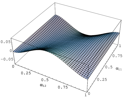
Figure 1: $H_{21}(\alpha_{11},\alpha_{12})$.

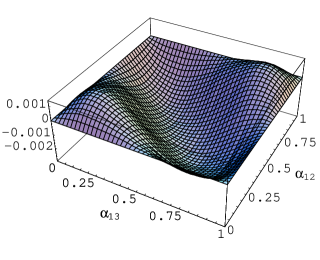
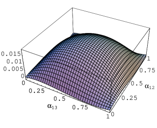
(a)	(b)
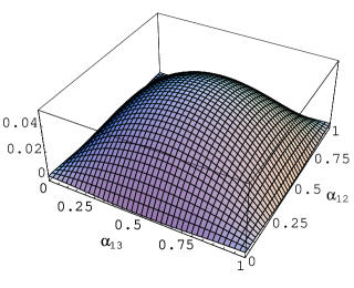
(c)

Figure 2: The mixed third virial coefficient $a_{111}(\alpha_{12},\alpha_{13},\alpha_{23})=-2H_{111}(\alpha_{12},\alpha_{13},\alpha_{23})$ at (a) $\alpha_{23}=0$, (b) $\alpha_{23}=0.1$, (c) $\alpha_{23}=0.5$.

We now turn to a direct numerical computation of the generating functions, and thence of the cluster and virial coefficients. To that end, we Monte Carlo simulate random paths inducing a given permutation, with the thermal distribution valid for free bosons. For each path, we calculate the intracycle and intercycle winding numbers as defined by Eqs. (3.3), (3.4). The resulting winding number probabilities are substituted into the definitions of the generating functions.

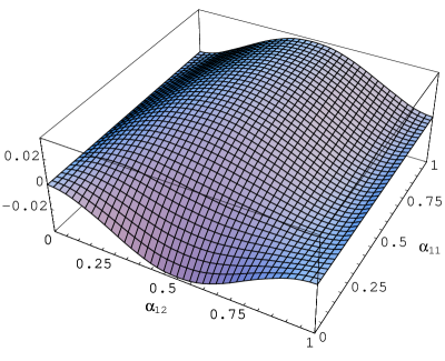
Figure 3: The mixed third virial coefficient $a_{21}(\alpha_{11},\alpha_{12})$.

We are interested in the thermodynamic limit, in which $Z_{1}^{-1}\to 0$; but in practice, the calculations have to be performed at a finite value of $Z_{1}^{-1}$, determined by the choice of $\beta$. (Both $m$ and $A$ can be scaled to unity, then $Z_{1}^{-1}=2\pi\beta$.) A compromise is necessarily involved: This value cannot be too big lest finite-size effects emerge, but it cannot be too small because, as explained above, the number of useful events tends to zero together with it. We have chosen such values (different for different partitions) that typically several paths out of a thousand contribute to the connected parts.

For the (21) partition, $32.1\times 10^{6}$ paths were generated at $\beta=0.01$ ($Z_{1}^{-1}=0.0628$). Figure 1 shows the correction $H_{21}(\alpha_{11},\alpha_{12})$ to the polynomial approximation $\tilde{G}_{21}$, Eq. (4.2). It vanishes, as it should, for $\alpha_{12}=0$ and $\alpha_{12}=1$ (no statistical interaction between the two species), as well as for $\alpha_{11}=\alpha_{12}$ (see above). Also, like $\tilde{G}_{21}$ itself, it is antisymmetric with respect to $(\alpha_{11},\alpha_{12})\mapsto(1-\alpha_{11},1-\alpha_{12})$, since the total winding number is always odd. The maximum is $H_{21}(0,0.5)\simeq 0.071$, which is to be compared with the maximum of $\tilde{G}_{21}(0,0.5)=0.500$; thus, the relative error of the two-particle approximation is about 15%. The absolute error of the MC data themselves, which can be estimated by looking at the imaginary part of the simulated function, never surpasses $0.001$.

For the (111) partition, $340\times 10^{6}$ paths were generated at $\beta=0.03$ ($Z_{1}^{-1}=0.188$). We illustrate our results with plots of $a_{111}(\alpha_{12},\alpha_{13},\alpha_{23})=-2H_{111}(\alpha_{12},\alpha_{13},\alpha_{23})$ at fixed values of $\alpha_{13}=0$, $0.1$, and $0.5$, on Fig. 2 (a), (b), (c), resp. The first of the three cases, where winding numbers of one of the pairs do not contribute, reflects the three-particle correlation in the windings of the pairs (12) and (13). The extreme value, $H_{111}(0.5,0.5,0)\simeq 0.00138$, is to be compared with the conditional maximum $\tilde{G}_{111}(0.5,0.5,0)=0.06250$. The approximation of uncorrelated windings per se is, therefore, accurate up to 2%. When all three parameters are nonzero, it is not only the above-mentioned correlation but also any paths with all three winding numbers nonvanishing that start to contribute to the correction, making the latter bigger by almost an order of magnitude. The extreme value is $H_{111}(0.5,0.5,0.5)\simeq-0.0252$ vs. $\tilde{G}_{111}(0.5,0.5,0.5)=0.1875$; the error is $0.00025$ at most. Correspondingly, the extreme value of the three-species mixed virial coefficient is $a_{111}(0.5,0.5,0.5)\simeq 0.0504$.

Our next result, Fig. 3, is the two-species mixed third virial coefficient $a_{21}(\alpha_{11},\alpha_{12})$, determined from Eq. (4.6). It includes an antisymmetric [with respect to $(\alpha_{11},\alpha_{12})\mapsto(1-\alpha_{11},1-\alpha_{12})$] part, $H_{21}$, and a symmetric one, $H_{111}$. The latter being mostly negative, the virial coefficient is predominantly positive; however, its extreme negative value, $a_{21}(0,0.5)\simeq-0.0368$ is slightly bigger by magnitude than its extreme positive value, $a_{21}(1,0.5)\simeq 0.0343$.

As a final check, we have computed the single-species third-order virial coefficient $a_{3}(\alpha_{11})$, and found the result to be consistent with the known formula [7],

$$a_{3}(\alpha)=\frac{1}{36}+\frac{1}{12\pi^{2}}\sin^{2}\pi\alpha-(1.65\pm 0.01)\times 10^{-5}\sin^{4}\pi\alpha\;,$$ (5.1)

within the error margin of $0.0002$. (The magnitude of the error is bigger than that of the $\sin^{4}$ term, which cannot therefore be seen here.)

The next logical step is to try to infer the approximate analytic formulas for the mixed virial coefficients, either as fits to the MC data or by somehow taking into account multiparticle correlations in the winding number distributions. It is possible to make some progress on both avenues; results will be reported elsewhere [14].

References

- [1] R. Sorkin, Phys. Rev. D27 (1983) 1787; G.A. Goldin, R. Menikoff, D.H. Sharp, Phys. Rev. Lett. 54 (1985) 603; F. Wilczek, Phys. Rev. Lett. 69 (1992) 132; A. Dasnières de Veigy, S. Ouvry, Phys. Lett. B307 (1993) 91.
- [2] J.M. Leinaas, J. Myrheim, Nuovo Cimento 37B (1977) 1; G.A. Goldin, R. Menikoff, D.H. Sharp, J. Math. Phys. 21 (1980) 650; J. Math. Phys. 22 (1981) 1664; F. Wilczek, Phys. Rev. Lett. 48 (1982) 1144; Phys. Rev. Lett. 49 (1982) 957.
- [3] D.P. Arovas, R, Schrieffer, F. Wilczek, Phys. Rev. Lett. 53 (1984) 722; H. Kjønsberg, J. Myrheim, Int. J. Mod. Phys. A14 (1999) 537.
- [4] S. Isakov, S. Mashkevich, S. Ouvry, Nucl. Phys. B448 (1995) 457.
- [5] S. Isakov, S. Mashkevich, Nucl. Phys. B504 (1997) 701.
- [6] M. Sporre, J.J.M. Verbaarschot, I. Zahed, Phys. Rev. Lett. 67 (1991) 1813; Phys. Rev. B46 (1992) 5738; Nucl. Phys. B389 (1993) 645; M.V.N. Murthy, J. Law, M. Brack, R.K. Bhaduri, Phys. Rev. Lett. 67 (1991) 1817.
- [7] S. Mashkevich, J. Myrheim, K. Olaussen, Phys. Lett. B382 (1996) 124.
- [8] J. Myrheim, Les Houches lecture notes (1998).
- [9] A. Kristoffersen, S. Mashkevich, J. Myrheim, K. Olaussen, Int. J. Mod. Phys. A13 (1998) 3723.
- [10] J. Myrheim, K. Olaussen, Phys. Lett. B299 (1993) 267.
- [11] M.D. Johnson, G.S. Canright, Phys. Rev. B49 (1994) 2947; S.B. Isakov, G.S. Canright, M.D. Johnson, Phys. Rev. B55 (1997) 6727.
- [12] J. Desbois, C. Heinemann, S. Ouvry, Phys. Rev. D51 (1995) 942; A. Dasnières de Veigy, Nucl. Phys. B458 (1996) 533, and private communication.
- [13] D.P. Arovas, R. Schrieffer, F. Wilczek, A. Zee, Nucl. Phys. B 251 (1985) 117.
- [14] S. Mashkevich, J. Myrheim, K. Olaussen, to be published.