Entanglement entropy of random quantum critical points in one dimension

Abstract

For quantum critical spin chains without disorder, it is known that the entanglement of a segment of $N\gg 1$ spins with the remainder is logarithmic in $N$ with a prefactor fixed by the central charge of the associated conformal field theory. We show that for a class of strongly random quantum spin chains, the same logarithmic scaling holds for mean entanglement at criticality and defines a critical entropy equivalent to central charge in the pure case. This effective central charge is obtained for Heisenberg, XX, and quantum Ising chains using an analytic real-space renormalization group approach believed to be asymptotically exact. For these random chains, the effective universal central charge is characteristic of a universality class and is consistent with a $c$-theorem.

Second-order phase transitions at zero temperature show universal scaling behavior determined by the collective physics of quantum fluctuations. Recently the scaling of the entanglement near such quantum critical points has been of special interest: at a quantum critical point, the length scale over which different regions of the system are entangled becomes divergent. The entanglement near criticality was shown to obey a universal scaling law in some one-dimensional (1D) systems. Most quantum phase transitions in pure 1D systems are invariant under local conformal transformations, and the entanglement at a critical point is related to the central charge of the associated conformal field theory Holzhey et al. (1994); Vidal et al. (2003).

Our primary result is that there exists universal entanglement scaling even for a class of disordered quantum critical points in one dimension that are not conformally invariant. The specific theories considered here describe random quantum spin chains: the Heisenberg, XX, and quantum Ising chains with random nearest-neighbor coupling have been previously found, Fisher (1994, 1995) using a real-space renormalization-group (RG) approach, to be described by strongly disordered critical points, as reviewed below.

The entanglement of a pure quantum-mechanical state $|\psi\rangle$ with respect to a partition into two subsystems $A$ and $B$ is the von Neumann entropy of the reduced density matrix for either subsystem:

$$S=-{\rm Tr}\rho_{A}\log_{2}\rho_{A}=-{\rm Tr}\rho_{B}\log_{2}\rho_{B}$$ (1)

where the reduced density matrix $\rho_{A}$ for subsystem $A$ is obtained by tracing over a basis $\phi_{B}^{i}$ of subsystem $B$

$$\langle\phi^{1}_{A}|\rho_{A}|\phi^{2}_{A}\rangle=\sum_{i}(\langle\phi^{1}_{A}|\times\langle\phi^{i}_{B}|)\psi\rangle\langle\psi(|\phi^{2}_{A}\rangle\times|\phi^{i}_{B}\rangle).$$ (2)

Note that this pure-state entanglement of a spin chain Vidal (2003) differs from the two-spin mixed-state entanglement Osterloh et al. (2002); Osborne and Nielsen (2002), which also has special behavior near a phase transition, but is only nonzero at short distances and is tied to the spin-spin correlator rather than the central charge Subrahmanyam (2004).

For conformally invariant critical theories in one dimension Holzhey et al. (1994), the entanglement of a finite region of size $L$ with the remainder of the system grows logarithmically in $L$ at a critical point, while away from criticality the entanglement is localized near the boundaries of the subsystem and goes to a constant for large $L$. For critical lattice models like quantum spin chains, the entanglement of a segment of $L$ sites with the remaining sites grows as $\log_{2}L$, with a coefficient determined by the central charge of the conformal field theory (CFT) Vidal (2003):

$$S_{N}\sim{c+{\bar{c}}\over 6}\log_{2}L.$$ (3)

Here $c$ and ${\bar{c}}$ are the holomorphic and antiholomorphic central charges of the CFT (for the cases we discuss $c={\bar{c}}$), which control several physical properties such as low-temperature specific heat. Slightly off criticality, the spin chain has a finite entanglement length $\xi$, and the entanglement saturates as $L\rightarrow\infty$ to $S\sim{c+{\bar{c}}\over 6}\log_{2}\xi.$

An example of a quantum spin chain that is critical without disorder is the antiferromagnetic Heisenberg model; the ground state of the spin-half chain

$$H=J\sum_{i}{\bf S}_{i}\cdot{\bf S}_{i+1}=J\sum_{i}(S^{z}_{i}S^{z}_{j}+\frac{S^{+}_{i}S^{-}_{j}+S^{-}_{i}S^{+}_{j}}{2})$$ (4)

is quantum critical for the antiferromagnetic case $J>0$. Staggered spin-spin correlations, $(-1)^{|i-j|}\langle{\bf S}_{i}\cdot{\bf S}_{j}\rangle$, fall off as $1/|i-j|$ up to logarithmic corrections.

The nature of quantum spin chains with quenched randomness at zero temperature is quite different from the above pure case. It is believed that any initial randomness in the distribution of couplings drives the system at long distances to a random quantum critical point: in RG language, disorder is a relevant perturbation to the pure critical points. This flow to strong disorder occurs for the Heisenberg chain, the XX chain, which has coupling only in two spin directions, and the quantum Ising chain, which has couplings in one spin direction plus a normal magnetic field (both made random).

The low energy properties of the random Heisenberg and XX models are described by the random singlet phase . This is shown using the real-space RG approach Ma et al. (1979); Dasgupta and Ma (1980); Fisher (1994). We review the real-space RG approach and the random singlet ground state, starting with the random Heisenberg Hamiltonian

$$H=\sum_{i}J_{i}{\bf S}_{i}\cdot{\bf S}_{i+1}.$$ (5)

The same results apply to the XX chain. In Eq. (5), $J_{i}$’s are drawn from any nonsingular distribution Fisher (1994).

The real-space RG analysis consists of iteratively finding the strongest bond, e.g. $J_{i}$, and diagonalizing it independently of the rest of the chain. This leads to a singlet between spins $i$ and $i+1$ in zeroth order (Fig 1a):

$$|\psi^{(0)}\rangle=|\psi_{x<i}\rangle\frac{1}{\sqrt{2}}\left(\left|\uparrow_{i}\downarrow_{i+1}\rangle\right.-\left|\downarrow_{i}\uparrow_{i+1}\rangle\right.\right)|\psi_{x>i+1}\rangle.$$ (6)

Next, we treat the rest of the Hamiltonian as a perturbation. If we begin with strong disorder (the distribution of $\ln J_{i}$ is wide), we can assume that $J_{i}\gg J_{i-1},\,J_{i+1}$, and use degenerate second order perturbation theory. This leads to a Heisenberg interaction between the neighboring spins at sites $i-1$ and $i+2$ with strength

$$\tilde{J}_{i-1,\,i+2}=\frac{J_{i-1}J_{i+1}}{2J_{i}}<J_{i-1},\,J_{i},\,J_{i+1}.$$ (7)

Thus we eliminate two sites, and reduce the Hamiltonian’s energy scale. Iterating these steps gives the ground state. Although this method is patently not correct when applied to a chain with little disorder, it is still applicable and is asymptotically correct at large distances. Fisher (1994)

Figure 1: a. RG decimation step: if $J_{i}$ is the strongest bond in the chain, sites $i$ and $i+1$ form a singlet (solid line); which diagonalizes $J_{i}{\bf S}_{i}\cdot{\bf S}_{i+1}$. Quantum fluctuations produce an effective interaction between sites $i-1$ and $i+2$ (dashed line). b. The random singlet ground state. Note that singlets may connect arbitrarily distant sites.

The RG leads to an integro-differential flow equation for the bond coupling distribution. This equation is best stated in terms of the logarithmic coupling strength $\beta=\ln\frac{\Omega}{J}$ and RG flow parameter $\Gamma=\ln\frac{\Omega_{0}}{\Omega}$, where $\Omega_{0}$ is the Hamiltonian’s initial energy scale, and $\Omega$ is its reduced energy scale. These variables capture the scaling properties of the problem; e.g., neglecting a $\ln 2$, Eq. (7) is simply $\tilde{\beta}_{i-1,\,i+2}=\beta_{i-1}+\beta_{i+1}$. Note that strongest bonds have $\beta=0$. In terms of $\beta$ and $\Gamma$ we haveFisher (1994)

$$\frac{dP_{\Gamma}(\beta)}{d\Gamma} = P_{\Gamma}(0)\int d\beta_{1}d\beta_{2}\delta(\beta_{1}+\beta_{2}-\beta)P_{\Gamma}(\beta_{2})P_{\Gamma}(\beta_{1})$$ (9)

$$+\frac{\partial P_{\Gamma}(\beta)}{\partial\beta}.$$

The following solution is an attractor to essentially all initial bond distributions, and it describes the low-energy behavior of the spin chain: Fisher (1994)

$$P(\beta)=\frac{1}{\Gamma}e^{-\beta/\Gamma}.$$ (10)

This is the random-singlet fixed point distribution.

The real space RG shows that the spin chain is in the random-singlet phase. In this phase singlets form in a random fashion over all length scales, and can connect spins arbitrarily far apart (Fig. 1b). Long-distance singlets form at low energy scales. On average,

$$\lambda\sim\Gamma^{2},$$ (11)

where $\lambda$ is the length scale of singlets forming at energy scale $\Omega=\Omega_{0}E^{-\Gamma}$. The long range of the low-energy singlets leads to slowly decaying average correlations, which for the random Heisenberg model decay algebraically, and not exponentially as one would expect from the localized nature of the random-singlet state.

Let us focus on the entanglement entropy of the random Heisenberg model. The entanglement of a spin-$1/2$ particle in a singlet with another such particle is $1$, which is the entropy of the two states of a spin with its partner traced out. The entanglement of a segment of the random Heisenberg chain is just the number of singlets that connect sites inside to sites outside the segment (Fig. 2).

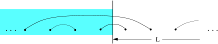
Figure 2: The entanglement entropy of a segment is the number of singlets that connect the segment with the rest of the chain (shaded area). In this example there are two such singlets.

To obtain the entanglement, we calculate the number, $N$, of singlets that form over a single bond $B$ (in the example above, we form singlets between sites $i$ and $i+1$, and later in the RG between sites $i-1$ and $i+2$, etc.). If (as a first approximation) we neglect the history dependence of the distribution of bond $B$, we can find $N$ by using the distribution of bond strengths, Eq. (10). When we change the energy scale $\Omega\rightarrow\Omega-d\Omega$, $\Gamma\rightarrow\Gamma+d\Gamma$, all bonds with $0<\beta<d\Gamma$ get decimated. The average number of decimations over bond $B$ grows by

$$d\overline{N}=d\Gamma P(\beta=0)=\frac{d\Gamma}{\Gamma}$$ (12)

which leads to $\overline{N}=\ln\Gamma$.

This picture breaks down once singlets exceed the size $L$ of the segment , when (by Eq. 11) $\Gamma=\sqrt{L}$. So the number of singlets emanating from the segment of size $L$, i.e. its entanglement with the rest of the chain, is

$$S_{L}\sim N_{L}\approx 2\cdot\ln\sqrt{L}+k=\ln L+k,$$ (13)

where $k$ is a nonuniversal constant, which also depends on the initial realization of the disorder.

Neglecting the history of $B$ allowed us to see simply why the entropy depends on $\ln L$, but the coefficient we obtained is not correct. To include the history of $B$, we note from Eqs. (7, 10) that the bond strength distribution of $B$ right after being decimated at $\Gamma_{0}$ is

$$Q(\beta)=\int d\beta_{1}d\beta_{2}\delta(\beta_{1}+\beta_{2}-\beta)P_{\Gamma_{0}}(\beta_{2})P_{\Gamma_{0}}(\beta_{1})=\frac{\beta}{\Gamma_{0}^{2}}e^{-\beta/\Gamma}.$$ (14)

Now we ask at what $\Gamma$ is $B$ decimated again. To answer this, we need a flow equation for $Q_{\Gamma}(\beta)$ similar to Eq. (9). In the following, we use the convention that $\int\limits_{0}^{\infty}d\beta Q_{\Gamma}(\beta)=p_{\Gamma}$ is the probability that bond $B$ was not yet decimated at scale $\Gamma$. With this convention in mind, $Q_{\Gamma}(\beta)$ obeys

$$\begin{array}[]{c}\frac{dQ_{\Gamma}(\beta)}{d\Gamma}=\frac{\partial Q_{\Gamma}(\beta)}{\partial\beta}-2Q_{\Gamma}(\beta)P_{\Gamma}(0)\vspace{2mm}\\ +2P_{\Gamma}(0)\int d\beta_{1}d\beta_{2}\delta(\beta_{1}+\beta_{2}-\beta)P_{\Gamma}(\beta_{2})Q_{\Gamma}(\beta_{1}).\end{array}$$ (15)

The first term is due to the change in $\beta$ when $\Omega$ changes, the second and third terms account for $B$’s flow due to one of its two neighbors forming a singlet. Note that $\frac{dp_{\Gamma}}{d\Gamma}=-Q_{\Gamma}(0)$. Eq. (15) can be solved using the ansatz:

$$Q_{\Gamma}(\beta)=\left(a_{\Gamma}+b_{\Gamma}\frac{\beta}{\Gamma}\right)P_{\Gamma}(\beta)$$ (16)

by substituting Eq. (16) in Eq. (15) we obtain

$$\begin{array}[]{cc}\frac{da_{\Gamma}}{dl}=\Gamma\frac{da_{\Gamma}}{d\Gamma}=b_{\Gamma}-2a_{\Gamma},&\frac{db_{\Gamma}}{dl}=\Gamma\frac{db_{\Gamma}}{d\Gamma}=-b_{\Gamma}+a_{\Gamma},\end{array}$$ (17)

with $l=\ln\Gamma/\Gamma_{0}$. Also $a_{\Gamma_{0}}=0,\,b_{\Gamma_{0}}=1$, from Eq. (14).

Next we calculate the rate of singlet formation over $B$. First, note that the survival probability $p_{\Gamma}$ obeys $p_{\Gamma}=a_{\Gamma}+b_{\Gamma}$ and depends on $\Gamma$ only through $l=\ln\Gamma/\Gamma_{0}$. Therefore the duration $l$ between two consecutive singlets forming on bond $B$ is independent of  $\Gamma_{0}$. This also proves that the number of singlets over $B$ is proportional to $\ln\Gamma$. To find the proportionality constant we calculate the average duration $\langle l\rangle$ between decimations; the number of bonds is then $N=\frac{\ln\Gamma}{\langle l\rangle}$. We have

$$\langle l\rangle=\int\,dp_{\Gamma}\,l=\int\limits_{0}^{\infty}\,dl\,a_{\Gamma}l.$$ (18)

From Eq. (17) one finds $a_{\Gamma}=\frac{1}{\sqrt{5}}\left(e^{-\frac{3-\sqrt{5}}{2}l}-e^{-\frac{3+\sqrt{5}}{2}l}\right).$ Inserting this in Eq. (18) we find $\langle l\rangle=3$. Therefore:

$$S_{L}=\frac{1}{3}\cdot 2\ln\Gamma+k=\frac{\ln 2}{3}\log_{2}L+k.$$ (19)

Hence the ’effective central charge’ of the random Heisenberg chain is ${\tilde{c}}=1\cdot\ln 2$, which is the central charge of the pure Heisenberg chain times an irrational number.

We discuss the interpretation and physical consequences of this effective central charge below, but first obtain its value for the quantum Ising case. The pure quantum Ising model has a well known ferromagnetic to paramagnetic phase transition. Its random analog is

$$H=-\sum_{i}J_{i}\hat{\sigma}^{z}_{i}\hat{\sigma}^{z}_{i+1}-\sum_{i}h_{i}\hat{\sigma}^{x}_{i},$$ (20)

where $h_{i}$ and $J_{i}$ are random, and $\sigma$ are spin-1/2 Pauli matrices. This model also has a ferromagnetic to paramagnetic phase transition, described by a random critical point similar to the random singlet phase Fisher (1995). Hence we expect entanglement in the quantum Ising case also to scale logarithmically with the size $L$ of the test segment.

As with the random Heisenberg case, we use real-space RG to study the ground state of the random quantum Ising model (Fig. 3a). Again we diagonalize the term with the largest energy scale in the Hamiltonian; if it is $-J_{i}\hat{\sigma}^{z}_{i}\hat{\sigma}^{z}_{i+1}$, we set sites $i$ and $i+1$ to point in the same direction, $|\psi\rangle_{i,i+1}=\alpha\left|\uparrow_{i}\uparrow_{i+1}\rangle\right.+\beta\left|\downarrow_{i}\downarrow_{i+1}\right.\rangle$, thus creating a ferromagnetic cluster. Quantum fluctuations yield an effective transverse field on the cluster,

$$h_{i,i+1}=\frac{h_{i}h_{i+1}}{J_{i}}\,\,\left(\ll h_{i},\,h_{i+1},\,J_{i}\right).$$ (21)

If the term with largest energy happens to be $-h_{i}\hat{\sigma}^{x}_{i}$, we set the $i$’th spin point in the $x$ direction, $|\psi\rangle_{i}=\left|\rightarrow_{i}\rangle\right.=\frac{1}{\sqrt{2}}\left(\left|\uparrow_{i}\rangle\right.+\left|\downarrow_{i}\rangle\right.\right)$, by which we decimate the $i$’th spin. Quantum fluctuations produce an effective Ising coupling between sites $i-1$ and $i+1$ with strength:

$$J_{i-1,i+1}=\frac{J_{i-1}J_{i}}{h_{i}}\,\,\left(\ll J_{i-1},\,J_{i},\,h_{i}\right).$$ (22)

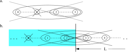
Figure 3: (a) Typical ground state in the random quantum Ising model. It formed as follows; sites $2$ and $3$ form a cluster, site $1$ is frozen in the $x$ direction, site $0$ joins the cluster of $2$ and $3$, and finally the large cluster is frozen along $x$. (b) The entanglement of a segment $L$ is given by the number of decimated clusters that connect the segment with the rest of the chain (shaded area). In this example there are two such clusters: sites $2$ and $3$, and sites $1$ and $4$.

The RG flow equations for the distributions of $h_{i}$ and $J_{i}$ as a function of $\Omega=\max\{J_{i},\,h_{i}\}$ support an attractor in which the logarithmic coupling distributions, $R(\zeta)$ and $P(\beta)$, with $\zeta=\ln\frac{\Omega}{J}$, $\beta=\ln\frac{\Omega}{h}$, are given by the random singlet expression in Eq. (10). As for the random singlet scaling, at criticality the absolute length $\lambda$ of the domains decimated by the transverse field scales as $\lambda\sim\Gamma^{2}$.

At low energy, larger and larger ferromagnetic clusters are formed and then decimated. For a segment of length $L$, ferromagnetic clusters which are completely within or completely outside the segment and decimated by the transverse field do not affect the entanglement. The only contributions come from ferromagnetic domains that cross the boundary of the segment (Fig. 3b), and each such cluster contributes $1$ to the entanglement.

Next we calculate how many ferromagnetic clusters are formed and decimated over an edge of the segment. At a given energy scale, the edge of the segment can either separate two unpaired sites, or be contained in a cluster which is partially in the segment (when such a cluster is decimated the edge returns to the first case). At the critical point these possibilities must occur with the same probability by a self-duality of the quantum Ising model (Fisher (1995); Refael and Fisher ). Hence the probability that the edge is in an active cluster at scale $\Gamma$ is $p=1/2$. By the analysis as for the Heisenberg chain, we obtain $N(\Gamma)=p\cdot\frac{1}{3}\ln\Gamma$, and

$$S_{L}=\frac{1}{6}\ln L+k=\frac{\ln 2}{6}\log_{2}L+k,$$ (23)

with $k$ a non-universal constant. The effective central charge of the random quantum Ising model is ${\tilde{c}}=1/2\cdot\ln 2$ - $\ln 2$ times the central charge in the pure system.

Eq. (23) shows that the critical quantum Ising chain has half the entanglement of the random singlet phase. But both of these are in the same infinite-randomness fixed point scaling category, so a difference in the entanglement entropy may seem surprising. However, these two systems also differ in their temporal correlations:

$$\overline{<\hat{\sigma}^{z}_{0}(0)\hat{\sigma}^{z}_{0}(\tau)>}\sim\frac{1}{\ln^{z}{\Omega_{0}\tau}},$$ (24)

with $z=2$ for the XXZ models and $z=1$ for the quantum Ising model. These two similar strong-randomness fixed points belong to different universality classes, and the effective central charge is sensitive to this difference.

For pure chains, the prefactors of correlation functions are non-universal but the central charge is universal. In the random case, non-universal correlation prefactors are generated by inaccuracies of the order of the lattice spacing in the location of the low energy effective spins; these occur when the RG scale $\Omega$ is still largeFisher and Young (1998). Such errors do not affect the universal coefficient of the logarithmic divergence of the entropy, but modify the additive non-universal ’surface term’ $k$ in Eqs. (19, 13). Note that entanglement is self-averaging as chain length $N\rightarrow\infty$.

The central charges we find for the random Heisenberg, XX, and quantum Ising chains are those of the pure models times $\ln 2$. Although irrational, these central charges are universal quantities which describe the universality class of the random chains. An example of the importance of $c$ in the pure case is the well known “$c$-theorem” Zamolodchikov (1986) that if an RG flow connects one critical point $A$ to another critical point $B$, then $c_{A}\geq c_{B}$. The values of ${\tilde{c}}$ obtained here for random systems suggest, given the relevance of disorder in these systems, that there is a generalized ${\tilde{c}}$-theorem based on entanglement even for nonconformal quantum critical points in 1D. This may imply constraints on the values of ${\tilde{c}}$ for spin chains obtained by, e.g., disordering higher-spin CFTs.

Since only certain rational values of $c$ are allowed for well-behaved CFTs with $c<1$, the irrational ${\tilde{c}}$ for random critical points is a fundamental difference between pure and random cases. This is reminiscent of the irrational residual entropy that appears in quantum impurity problems and satisfies a “$g$-theorem.” Affleck and Ludwig (1993)

The ratio between the random and pure values of ${\tilde{c}}$ is unexpectedly the same for all the different chains we studied. Perhaps $\tilde{c}$ of any random fixed point derived from a pure conformally invariant point is the product of the central charge of the pure theory and a universal number determined by the flow from the pure to the random fixed point. Numerics on the random $XX$ model via its free-fermion representation could determine whether ${\tilde{c}}$ appears as a universal amplitude as in the clean case for quantities beyond entanglement. It is clear already that the universal logarithmic scaling of entanglement provides a powerful way to characterize both pure and random quantum critical points in one dimension.

We gratefully acknowledge useful conversations with L. Balents, A. Kitaev, A. W. W. Ludwig, J. Preskill, and G. Vidal, and support from NSF PHY99-07949, DMR-0238760, and the Hellman Foundation.

References

- Holzhey et al. (1994) C. Holzhey, F. Larsen, and F. Wilczek, Nucl. Phys. B 424, 443 (1994).
- Vidal et al. (2003) G. Vidal, J. I. Latorre, E. Rico, and A. Kitaev, Phys. Rev. Lett. 90, 227902 (2003).
- Fisher (1994) D. S. Fisher, Phys. Rev. B 50, 3799 (1994).
- Fisher (1995) D. S. Fisher, Phys. Rev. B 51, 6411 (1995).
- Vidal (2003) G. Vidal, Phys. Rev. Lett. 91, 147902 (2003).
- Osterloh et al. (2002) A. Osterloh, L. Amico, G. Falci, and R. Fazio, Nature 416, 608 (2002).
- Osborne and Nielsen (2002) T. J. Osborne and M. A. Nielsen, Phys. Rev. A 66, 032110 (2002).
- Subrahmanyam (2004) V. Subrahmanyam, Phys. Rev. A 69, 022311 (2004).
- Ma et al. (1979) S. K. Ma, C. Dasgupta, and C. K. Hu, Phys. Rev. Lett. 43, 1434 (1979).
- Dasgupta and Ma (1980) C. Dasgupta and S. K. Ma, Phys. Rev. B 22, 1305 (1980).
- (11) G. Refael and D. S. Fisher, eprint cond-mat/0308176.
- Fisher and Young (1998) D. S. Fisher and A. P. Young, Phys. Rev. B 58, 9131 (1998).
- Zamolodchikov (1986) A. B. Zamolodchikov, JETP Lett. 43, 730 (1986).
- Affleck and Ludwig (1993) I. Affleck and A. W. W. Ludwig, Phys. Rev. B 48, 7297 (1993).