Quantum and semiclassical study of magnetic anti-dots

Abstract

We study the energy level structure of two-dimensional charged particles in inhomogeneous magnetic fields. In particular, for magnetic anti-dots the magnetic field is zero inside the dot and constant outside. Such a device can be fabricated with present-day technology. We present detailed semiclassical studies of such magnetic anti-dot systems and provide a comparison with exact quantum calculations. In the semiclassical approach we apply the Berry-Tabor formula for the density of states and the Borh-Sommerfeld quantization rules. In both cases we found good agreement with the exact spectrum in the weak magnetic field limit. The energy spectrum for a given missing flux quantum is classified in six possible classes of orbits and summarized in a so-called phase diagram. We also investigate the current flow patterns of different quantum states and show the clear correspondence with classical trajectories.

I Introduction

In the past decade, the study of systems of two-dimensional electron gas (2DEG) in semiconductorsHouten has been extended by the application of spatially inhomogeneous magnetic fields. The inhomogeneity of the magnetic field can be realized experimentally either by varying the topography of the electron gas Foden:cikk ; Leadbeater-1:cikk , by using ferromagnetic materials Leadbeater-2:cikk ; Krishnan:cikk ; Nogaret-1:cikk ; Nogaret-2:cikk ; Nogaret-4:cikk ; Nogaret-3:cikk , depositing a superconductor on top of the 2DEG Smith:cikk ; Geim:cikk . Numerous theoretical works also show an increasing interest in the study of electron motion in inhomogeneous magnetic field (see, e.g., Refs. Muller-1:cikk, ; Khveshchenko:cikk, ; Gotz:cikk, ; Peeters-1:cikk, ; Calvo:cikk, ; Peteers-2:cikk, ; Schmelcher:cikk, ; Matulis:cikk, ; Nielsen:cikk, ; Peteers-3:cikk, ; Sim:cikk, ; Urbach:thesis, ; Kim-1:cikk, ; Michele_Boese:cikk, ; Kim-2:cikk, ; Kim-3:cikk, ; Peteers-4:cikk, ; Peteers-5:cikk, ; Klaus_spin-orbit:cikk, ; IMB:cikk, ).

In the experimental works mentioned above, for GaAs heterostructures, on the one hand, the electron dynamics is confined to two-dimensions. On the other hand, the coherence length and the mean free path of the electron can be much larger than the size of the system, while the Fermi wavelength is comparable to the size of the 2DEG. Moreover, the electron system can be described to a good approximation as a free electron gas with an effective massHouten . Therefore, the quantum mechanical treatment of these systems is of some physical interest.

In this paper, as an example, we consider the energy levels of a two-dimensional non-interacting electron gas in a magnetic field that is zero inside a circular region and constant outside. This system (shown in Fig. 1) will be called a magnetic anti-dot; it was first studied by Solimany and Kramer Solimany . Solving the Schrödinger equation it was shown that there are bound states. Introducing an effective angular momentum, the Schrödinger equation of the particle in symmetric gauge can be mapped to the Landau model. This effective angular momentum is a sum of the angular momentum in a uniform magnetic field and the flux (in units of the flux quantum) missing from the uniform field. Recently, Sim et al. Sim:cikk have renewed the study of this system and pointed out the crucial role of the magnetic edge states in the magnetoconductance. The classical counterparts of these states correspond to trajectories of the charged particle that consist of straight segments inside the non-magnetic region and arcs outside.

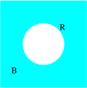
Figure 1: The two-dimensional electron gas in an inhomogeneous magnetic field. The magnetic field is zero inside the circle of radius $R$ and constant outside the circle.

Although it is difficult to measure directly the density of states of a quantum system, it affects many observable quantities such as the magnetoconductance, the magnetization or the susceptibility. In the interpretation of the experimental results the semiclassical approximation proved to be a useful tool. Several semiclassical approaches WKB:cikk ; Keller:cikkek ; Berry-Tabor:cikk ; Balian_Bloch:cikkek ; Gutzwiller:cikkek ; Strutinsky:cikkek ; Creagh_Littlejohn:cikk are known in the literature and an excellent overview of the subject can be found in the textbook by Brack and BhaduriBrack:book . Different semiclassical theories for magnetic systems have successfully been applied, for example, in works Blaschke:cikk ; Klaus_H ; Klama ; Klama-2 . For integrable systems Berry and Tabor Berry-Tabor:cikk have shown that the oscillating part of the density of states can always be expressed in terms of classical periodic orbits. This formula is commonly called the Berry-Tabor trace formula.

One of our aims in this paper is to apply, for the first time, the Berry-Tabor trace formula for a magnetic anti-dot. To illustrate the power of the method, we also calculate the exact eigenvalues of the single particle Schrödinger equation and find a very good agreement between the two results. We should mention here that the statement by Sim et al. Sim:cikk on the relation between the quantum states and the corresponding periodic orbits is somewhat misleading. Their condition for a given periodic orbit is not necessarily satisfied at the value of the corresponding exact energy level as they claimed However, including more and more periodic orbits with the proper weights in the trace formula the sum converges to the correct quantum density of states. In practice only a few of the shortest orbits are enough to get a rough estimate of the positions of the exact energy levels.

The power of the semiclassical approach can also be demonstrated by applying the Bohr-Sommerfeld approximation. We shall show that the energy levels obtained from the Bohr-Sommerfeld quantization rules also agree very well with the numerically exact levels even for the lowest eigenstates. Note that in this semiclassical treatment the quantization should be applied to the classical motion on a two-dimensional torus parametrized by the action variables and their canonically conjugate angle variables (for details see, eg, Ref. Brack:book, ).

The classical orbits can be classified by their cyclotron radius $\varrho$ and their guiding center $c$ (distance of the center of the orbits from the origin). In the quantum mechanical treatment one can calculate the average of operators defining the cyclotron radius and the guiding center. For circular magnetic billiards, Lent Lent:cikk has derived approximate expressions for these averages for a given quantum state. Following Ref. Lent:cikk, , one may derive the corresponding relations for magnetic anti-dot systems. Thus, these relations are the basis for classifying the different quantum states in terms of classical orbits for our system. We will show that the quantum states can be described by six different types of classical orbits. In addition, this classification enables us to draw a so-called ‘phase diagram’ which shows a clear one-to-one correspondence between classical orbits and quantum states.

To complete our semiclassical study, we finally present results for the probability current density calculated from quantum calculations. We shall argue that the current flow patterns can be understood qualitatively from the corresponding classical trajectories. Recently, Halperin Halperin:cikk has been shown that the total current (the integral of the current density along the radial direction) can be related to the dispersion of the energy levels (their angular momentum dependence). As it will be shown this general relation works in our magnetic anti-dot system, too.

Regarding the numerical calculations, we should mention that the semiclassical approach presented in this paper proves to be a very effective method. Moreover, it provides a better understanding of the nature of the quantum system. Our semiclassical method applied to magnetic anti-dot systems may be an important tool to understand the role of the magnetic edge states in the density of states or the magnetization (both are experimentally accessible physical qauntities). We believe that our semiclassical analysis can be extended to other types of inhomogeneous magnetic fields such as studied, eg, in Refs. Nogaret-1:cikk, ; Nogaret-2:cikk, ; Nogaret-4:cikk, ; Nogaret-3:cikk, as well as non-circular dot systems.

The rest of the text is organized as follows. In Sec. II the exact quantization condition (secular equation) is derived from the matching conditions of the wave functions at the boundary of the magnetic and non-magnetic regions. In Sec. III the semiclassical approximation is presented including the description of the classical motion of the particle in Subsec. III.1, the characterization of the possible periodic orbits in Subsec. III.2, some numerical results in Subsec. III.3, and the phase diagram in Subsec. III.4. The current flow patterns of the system are discussed in Sec. IV. Finally, the conclusions are given in Sec. V.

II Quantum calculation

In this section, we present the quantum mechanical treatment of the magnetic anti-dot. The magnetic field with a constant $B$ outside a circle of radius $R$ is assumed to be perpendicular to the plane of the 2DEG. The Hamiltonian of the electron of mass $M$ and charge $e$ is given by

$$H=\left\{\begin{array}[]{ll}\frac{{\bf p}^{2}}{2M},&{\rm if}\,\,\,\,r<R,\\[8.61108pt] \frac{{\left({\bf p}-e{\bf A}\right)}^{2}}{2M},&{\rm if}\,\,\,\,r>R,\end{array}\right.$$ (1)

where ${\bf p}$ is the canonically conjugate momentum, and the vector potential in polar coordinates $(r,\varphi)$ and symmetric gauge is given by Solimany

$${\bf A} = A_{\varphi}(r,\varphi)\,\hat{{\bf e}}_{\varphi},\,\,\,\text{where}$$ (2)

$$A_{\varphi}(r,\varphi) = B\,\frac{r^{2}-R^{2}}{2r}\,\Theta(r-R),$$

and $\hat{{\bf e}}_{\varphi}$ is the unit vector in the $\varphi$ direction. Here $\Theta(x)$ is the Heaviside step function.

The energy levels of the system are the eigenvalues $E$ of the Schrödinger equation:

$$\hat{H}\Psi(r,\varphi)=E\Psi(r,\varphi).$$ (3)

Rotational symmetry of the system implies a separation ansatz for the wave function as a product of radial and angular parts. We choose for the angular part the appropriate angular momentum eigenfunctions $e^{im\varphi}$ with quantum number $m$ (here $m$ is an integer). Thus the wave function for a given $m$ is separated as $\Psi(r,\varphi)=f_{m}(r)e^{im\varphi}$, where the radial wave functions $f_{m}(r)$ satisfy a one-dimensional Schrödinger equation in the normal region:

$$\hat{h}_{m}(\tau)f_{m}(\tau)=\varepsilon f_{m}(\tau),$$ (4a)

in which the radial Hamiltonian takes the form

$$\hat{h}_{m}(\tau)=-\frac{\partial^{2}}{\partial\tau^{2}}-\frac{1}{\tau}\frac{\partial}{\partial\tau}+V_{m}(\tau).$$ (4b)

Here we introduce the dimensionless variable $$\tau=r/l l=\sqrt{\hbar/|eB|} \omega_{c}=|eB|/M \varepsilon=2E/(\hbar\omega_{c})$$, where is the magnetic length, is the cyclotron frequency, is the dimensionless energy, and the radial potential is given by

$$V_{m}(\tau) = \left\{\begin{array}[]{ll}\frac{m^{2}}{\tau^{2}},&{\rm if}\,\,\,\,r<R,\\[8.61108pt] \frac{{\left(\frac{\tau^{2}}{2}-m_{\rm eff}\right)}^{2}}{\tau^{2}},&{\rm if}\,\,\,\,r>R,\end{array}\right.$$ (4e)

$$m_{\rm eff} = s+m\,\rm{sgn}(eB),$$ (4f)

where $s=R^{2}/(2l^{2})=\Phi/\Phi_{0}$ is the magnetic flux $\Phi=BR^{2}\pi$ (in units of the magnetic flux quantum $\Phi_{0}=h/\left|e\right|$) missing inside the circle of radius $R$. The function $\rm{sgn}\{\cdot\}$ stands for the sign function. In the numerical results presented in this paper, we always assume that the particle is an electron moving in a magnetic field along the positive $z$-axis, i.e., $\rm{sgn}(eB)=-1$. However, our theoretical results are not restricted in such a way.

Introducing the new variable $\xi=\tau^{2}/2$ and transforming the wave functions in the magnetic region ($r>R$) as

$$f_{m}(\tau)=\xi^{\mid m_{\rm eff}\mid/2}\,e^{-\xi/2}\,\chi_{m}(\xi),$$ (5)

Eq. (4a) results in a Kummer differential equation Abramowitz

$$\xi\frac{d^{2}\chi_{m}}{d\xi^{2}}+\left(1+\mid m_{\rm eff}\mid-\xi\right)\frac{d\chi_{m}}{d\xi}$$

$$-\frac{1+\mid m_{\rm eff}\mid-m_{\rm eff}-\varepsilon}{2}\chi_{m} = 0.$$ (6)

Thus the ansatz for the radial wave function in the magnetic region can finally be written as

$$f_{m}(\tau)=\xi^{\mid m_{\rm eff}\mid/2}\,e^{-\xi/2}$$ (7)

$$\times\,U\left(\frac{1+\mid m_{\rm eff}\mid-m_{\rm eff}-\varepsilon,}{2},1+\mid m_{\rm eff}\mid,\xi\right),$$

where $U$ is the confluent hypergeometric function Abramowitz . Note that the function $U$ tends to zero as $r\rightarrow\infty$.

It is easy to show that the radial wave function inside the circle of radius $R$ (where the magnetic field is zero) satisfies the Bessel differential equationAbramowitz . Thus the radial wave function is given by

$$g_{m}(\tau)=J_{m}(\sqrt{\epsilon}\,\tau),$$ (8)

where $J_{m}(x)$ is the Bessel function of order $m$.

Matching the radial wave functions inside and outside the circle gives a secular equation whose solutions are the eigenvalues of the system. The matching conditions at $r=R$ yield

$$\frac{d}{d\tau}\,\ln g_{m}(\tau)\,\rule[-6.88889pt]{0.2pt}{17.22217pt}\;\raisebox{-6.45831pt}{$\scriptstyle\tau=R/l$}=\frac{d}{d\tau}\,\ln f_{m}(\tau)\,\rule[-6.88889pt]{0.2pt}{17.22217pt}\;\raisebox{-6.45831pt}{$\scriptstyle\tau=R/l$}.$$ (9)

For a given $m$ this secular equation depends only on the dimensionless missing flux $s$.

III Semiclassical approximation: the Berry-Tabor approach

We now turn to the semiclassical treatment of the system. Generally, in $d$ dimensions, a system is integrable if there are $d$ independent constants of the motion. Usually this is the result of the separability of the Hamiltonian: In a suitably chosen coordinate system the Hamiltonian depends only on separate functions $\phi_{i}(q_{i},p_{i})$ of the coordinates and the conjugate momenta. This means that the dynamics can be viewed as a collection of independent one dimensional dynamical systems. The function $\phi(q_{i},p_{i})$ plays the role of the Hamiltonian in each subsystem. The one dimensional semiclassical quantization procedure can be carried out in each subsystem separately

$$I_{i}=\frac{1}{2\pi}\oint p_{i}dq_{i}=\hbar\left(n_{i}+\frac{\nu_{i}}{4}\right),\;\;\;n_{i}=0,1,2,...,$$ (10)

where $I_{i}$ is the action variable and $\nu_{i}$ is the Maslov index (for details see, eg, Ref. Brack:book, ). The Maslov index is the sum of the Maslov indices of the turning points of the classical motion. Smooth or “soft” classical turning points (zeros of $p_{i}(q_{i})$) contribute $+1$ to the Maslov index, while “hard” classical turning points (infinite potential walls) contribute $+2$. Equation (10), the Bohr-Sommerfeld quantization condition, is widely used to approximate the energy levels of classically integrable systems.

Alternatively, from Eq. (10) a semiclassical trace formula known as the Berry-Tabor formula Berry-Tabor:cikk can be derived for the oscillating part of the density of states. For two-dimensional systems, this formula can be written as

$$d(E) = d_{0}(E)$$ (11)

$$+\sum_{p}\sum_{j=1}^{+\infty}\frac{\cos\left({\frac{jS_{p}(E)}{\hbar}}-\frac{\pi}{2}j\nu_{p}+\frac{\pi}{4}\right)}{\pi\hbar^{3/2}\sqrt{\frac{j(n_{2,p})^{3}}{T_{p}^{2}}\,\frac{\partial^{2}g}{\partial I_{1}^{2}}}},$$

(for the detailed derivation of this expression see Appendix A). Here $d_{0}(E)$ is the average density of states. The $p$-summation runs over the primitive periodic orbits of the system, the $j$-summation runs over their repetitions; $S_{p},T_{p}$ and $\nu_{p}$ denote the classical action, the time and the Maslov-index of orbit $p$, respectively; $n_{2,p}$ is the number of cycles in the motion projected to the action variable $I_{2}$ under one cycle of the orbit; and $I_{1}=g(I_{2},E)$ denotes the action variable $I_{1}$ as a function of the energy and $I_{2}$.

III.1 Classical dynamics of the system

It is easy to show that the classical Hamiltonian in polar coordinates $(r,\varphi)$, inside and outside the non-magnetic region is:

$$H=\frac{p_{r}^{2}}{2M}+V(r),$$ (12)

where $p_{r}$ and $p_{\varphi}$ are the canonically conjugate momenta, and the radial potential $V(r)=\frac{\hbar\omega_{c}}{2}\,V_{m}(\tau)$ is the same as in (4e) with the following replacements:

$$m = \frac{p_{\varphi}}{\hbar},$$ (13a)

$$m_{\rm eff} = s+\frac{p_{\varphi}}{\hbar}\,\rm{sgn}(eB).$$ (13b)

Note that here $m$ and $m_{\rm eff}$ are continuous classical variables. As we shall see below in the semiclassical approximation, the canonical momentum $p_{\varphi}$ is quantized according to the Bohr-Sommerfeld quantization rules (10).

Since the Hamiltonian does not depend explicitly on $\varphi$ (the system is rotationally invariant), the conjugate momentum $p_{\varphi}$ is a constant of motion. Thus the angular action variable becomes

$$I_{\varphi}=\frac{1}{2\pi}\,\oint p_{\varphi}\,d\varphi=p_{\varphi}.$$ (14)

The conjugate momentum inside the anti-dot is in fact the angular momentum. Outside the anti-dot there is an additional term due to the non-zero vector potential. From $\dot{\varphi}=\partial H/\partial p_{\varphi}$ one finds

$$p_{\varphi}=\left\{\begin{array}[]{lr}Mr^{2}\dot{\varphi},&{\rm if}\,\,\,\,r<R,\\[8.61108pt] Mr^{2}\dot{\varphi}+eB\,\frac{r^{2}-R^{2}}{2},&{\rm if}\,\,\,\,r>R.\end{array}\right.$$ (15)

We now choose $I_{1}\equiv I_{r}$ and $I_{2}\equiv I_{\varphi}$ in Eq. (10). To calculate the radial action variable $I_{r}=g(I_{\varphi},E)$ one needs to perform the integral of $p_{r}=\sqrt{E-V(r)}$ between the classical turning points of the radial potential. For a given $E$ these turning points can be obtained from $V(r)=E$. Using the same dimensionless variables as in Sec. II, we have one turning point for the potential inside the non-magnetic circle:

$$\tau_{0}^{\rm in}=\frac{m}{\sqrt{\varepsilon}},$$ (16a)

and for the potential valid outside the circle there are two turning points:

$$\tau_{1,2}^{\rm out}=\sqrt{2(\varepsilon+m_{\rm eff})\mp 2\sqrt{\varepsilon(\varepsilon+2m_{\rm eff})}}$$ (16b)

$$= \!\!\sqrt{\varepsilon+m_{\rm eff}+\left|m_{\rm eff}\right|}\mp\sqrt{\varepsilon+m_{\rm eff}-\left|m_{\rm eff}\right|},$$

where the upper/lower sign of $\mp$ distinguishes the first and second turning points. Note that $\tau_{1}^{\rm out}<\tau_{2}^{\rm out}$, and the turning points are real if either $m_{\rm eff}>0$ or $\varepsilon\geq-2\,m_{\rm eff}$ for $m_{\rm eff}<0$.

For a given energy $E$ and momentum $p_{\varphi}$ one can calculate the cyclotron radius $\varrho$ and the guiding center $c$:

$$\varrho = l\,\sqrt{\varepsilon},$$ (17a)

$$c = l\,\sqrt{\varepsilon+2\,m_{\rm eff}}.$$ (17b)

The derivation in the frame of classical mechanics is outlined in Appendix B. Following Ref. Lent:cikk, the relation between these quantities and the corresponding quantum states of the system can be derived from quantum mechanics. It turns out that the same relations hold for the cyclotron radius and the guiding center provided $p_{\varphi}$ is quantized as $p_{\varphi}=\hbar m$, where $m$ now is an integer. Then, $m_{\rm eff}$ is the same as that defined by Eq. (4f). The same results were found by Sim et al. Sim:cikk . Using Eq. (17) we shall discuss in detail the correspondence between classical orbits and quantum states in Secs. III.4 and IV.

The turning points given in Eq. (16b) can be expressed in terms of the cyclotron radius and the guiding center:

$$l\,\tau_{1}^{\rm out} = \left\{\begin{array}[]{ll}c-\varrho,&\text{if}\,\,\,m_{\rm eff}>0,\\[4.30554pt] \varrho-c,&\text{if}\,\,\,m_{\rm eff}<0,\end{array}\right.$$ (18c)

$$l\,\tau_{2}^{\rm out} = c+\varrho.$$ (18d)

We can now classify the classical orbits according to the relation between the values of the turning points given by (16) and the corresponding radius of the circular non-magnetic region (in units of $l$)

$$\tau_{\rm R}=\frac{R}{l}=\sqrt{2s}.$$ (19)

There are two different cases listed in Table 1. For orbits of type $A$ the particle outside the non-magnetic region moves along a cyclotron orbit and then passes through the magnetic field free region as a free particle. In the case of orbits of type $B$ the particle does not penetrate the non-magnetic region. In this case one can further distinguish two additional types of cyclotron orbits depending on the sign of $m_{\rm eff}$. The condition $\tau_{1}^{\rm out}>\tau_{\rm R}$ listed in Table 1 and Eq. (18c) imply that $c-\varrho>R$ for $m_{\rm eff}>0$, and $\varrho-c>R$ for $m_{\rm eff}<0$. From a simple geometrical consideration it follows that in the first case the cyclotron orbits (denoted by $B_{1}$) lie outside the circle of radius $R$, while in the latter case the orbits (denoted by $B_{2}$) completely encircle the non-magnetic region. These conditions can be rewritten as

$$m\,{\rm sgn}(eB) > \sqrt{2\,s\,\varepsilon}>0,\,\,\,\text{for}\,\,\,B_{1},$$ (20a)

$$-m\,{\rm sgn}(eB) > \sqrt{2\,s\,\varepsilon}>0,\,\,\,\text{for}\,\,\,B_{2}.$$ (20b)

For both types $B_{1}$ and $B_{2}$, $\varepsilon<m^{2}/2s$ is valid. In the case of orbits of type $A$ we have $\varepsilon>m^{2}/2s$.

We now turn to the calculation of the radial action variable $I_{r}$. Using the radial potential given by (4e) inside the non-magnetic circle we find

$$\Theta_{\rm in}(\varepsilon,\tau)\equiv\frac{1}{\hbar}\,\int p_{r}\,dr=\int\sqrt{\varepsilon-V(\tau)}\,d\tau$$ (21a)

$$= \sqrt{\varepsilon\tau^{2}-m^{2}}-m\,\arccos\,\frac{m}{\tau\,\sqrt{\varepsilon}},$$

and similarly outside, we have

$$\Theta_{\rm out}(\varepsilon,\tau)\equiv\frac{1}{\hbar}\,\int p_{r}\,dr=\int\sqrt{\varepsilon-V(\tau)}\,d\tau$$ (21b)

$$= \frac{1}{2}\,\sqrt{\varepsilon\,\tau^{2}-\left(\frac{\tau^{2}}{2}-m_{\rm eff}\right)^{2}}$$

$$-\frac{1}{2}\,(\varepsilon+m_{\rm eff})\arcsin\left(\frac{\varepsilon+m_{\rm eff}-\tau^{2}/2}{\sqrt{\varepsilon\left(\varepsilon+2m_{\rm eff}\right)}}\right)$$

$$-\frac{1}{2}\,|m_{\rm eff}|\arcsin\left(\frac{\tau^{2}(\varepsilon+m_{\rm eff})-2m_{\rm eff}^{2}}{\tau^{2}\sqrt{\varepsilon\left(\varepsilon+2m_{\rm eff}\right)}}\right).$$

The radial action variables for the orbits of types $A$ and $B$ can be expressed in terms of the functions $\Theta_{\rm in}$ and $\Theta_{\rm out}$, and are listed in Table 1.

Table 1: Classification of the orbits and the corresponding radial action variables. See also the text.

Case	conditions	$\frac{\pi}{\hbar}\,I_{r}$
$A$	$\tau_{0}^{\rm in}\leq\tau_{\rm R}$ and	$\Theta_{\rm out}(\varepsilon,\tau_{2}^{\rm out})-\Theta_{\rm out}(\varepsilon,\tau_{\rm R})$
	$\tau_{2}^{\rm out}>\tau_{\rm R}$	$+\,\Theta_{\rm in}(\varepsilon,\tau_{\rm R})-\Theta_{\rm in}(\varepsilon,\tau_{0}^{\rm in})$
$B$	$\tau_{1}^{\rm out}>\tau_{\rm R}$	$\Theta_{\rm out}(\varepsilon,\tau_{2}^{\rm out})-\Theta_{\rm out}(\varepsilon,\tau_{1}^{\rm out})$

Note that

$$\Theta_{\rm out}(\varepsilon,\tau_{1}^{\rm out}) = -\frac{\pi}{4}\,\left(\varepsilon+m_{\rm eff}-\left|m_{\rm eff}\right|\right),$$ (22a)

$$\Theta_{\rm out}(\varepsilon,\tau_{2}^{\rm out}) = -\Theta_{\rm out}(\varepsilon,\tau_{1}^{\rm out}).$$ (22b)

Thus, for orbits of type $B$, the radial action variable $I_{r}$ can be simplified to

$$I_{r}=\frac{\hbar}{2}\,\left(\varepsilon+m_{\rm eff}-\left|m_{\rm eff}\right|\right).$$ (23)

It is clear from (14) and Table 1 that for fixed $s$, the radial action variable $I_{r}$ is a function of the rescaled energy $\varepsilon$ and the angular action variable $I_{\varphi}$ through $m$ and $m_{\rm eff}$. Then, for orbits of type $A$, the partial derivative in the denominator of Eq. (11) has a rather simple form

$$\hbar\,\frac{\partial^{2}I_{r}}{\partial I_{\varphi}^{2}}=\frac{1}{\pi\,\sqrt{2\,s\,\varepsilon-m^{2}}}\,\frac{s+m_{\rm eff}}{\varepsilon+2\,m_{\rm eff}}.$$ (24)

However, the amplitude for orbits of type $B$ in Eq. (11) cannot be calculated using the second partial derivative of $I_{r}$, therefore the contribution from these orbits to the semiclassical level density is calculated separately in Appendix C.

Knowing the explicit $\varepsilon$ and $I_{\varphi}$ dependence of the radial action variable $I_{r}$, the Bohr-Sommerfeld quantization conditions given by Eq. (10) for orbits of type $A$ can be rewritten as

$$I_{\varphi} = \hbar\,m,$$ (25a)

$$I_{r} = \hbar\left(n+\frac{1}{2}\right),$$ (25b)

where $$n=0,1,2,\cdots m I_{r} \nu_{\varphi}=0 \nu_{r}=2 B$$ and is an integer, and the energy-dependent radial action variable is given in Table 1 (the Maslov indices are and , for details see, eg, Ref. Brack:book, ). Using (23) for orbits of type , the semiclassical quantization conditions can be simplified and the energy levels are

$$E_{m,n}=\hbar\,\omega_{c}\,\left(n+\frac{\left|m_{\rm eff}\right|-m_{\rm eff}+1}{2}\right),$$ (25c)

where $m_{\rm eff}=s+m\,{\rm sgn}(eB)$, and $m$ and $n$ are integers. These levels coincide with the familiar Landau levels in a homogeneous magnetic field but the quantum number $m$ is replaced by $m_{\rm eff}$. Below in Sec. III.3 we shall compare the exact energy levels with those obtained from the Bohr-Sommerfeld quantization conditions for orbits of types $A$ and $B$.

III.2 Periodic orbits

To apply the Berry-Tabor formula (11), one needs to describe the possible periodic orbits of the magnetic anti-dot system. The periodic orbits of type $A$ can be characterized by their winding number $w$ (the number of turns around the center under one cycle) and the number of identical orbit segments $n_{s}$ the orbit can be split up to. These segments consist of a circular path outside the anti-dot followed by a straight line inside. We introduce the angles $\alpha,\beta$ and $\gamma$ to characterize these basic orbit segments as shown in Fig. 2.

Figure 2: Two examples for the basic orbit segments (an arc in the magnetic field followed by a straight line inside the anti-dot) of orbit type $A$, and the related angles $\alpha,\beta$ and $\gamma$. A particle traveling along the segments moves anti-clockwise with respect to the center of the anti-dot in the case drawn on the left, while in the other example it moves clockwise on the straight line inside the anti-dot. Thus in this case the angle $\gamma$ is negative.

These angles always fulfill

$$n_{s}(\beta+\gamma) = w\pi,$$ (26a)

$$\frac{\sin(\alpha)}{\sin(\beta)} = \frac{R}{\rho},$$ (26b)

($\alpha$ and $\beta$ are always positive and the sign of $\gamma$ follows the sign of $w$). The relations between the indices $w,n_{s}$ and the angles characterizing the basic orbit segment are summarized in Table 2 for the four possible sub-classes. When either $w$ is negative (orbits of type $A{}_{1}$), or the cyclotron radius $\rho$ is smaller than the radius of the anti-dot (orbits of type $A{}_{2}$), the angles $\alpha,\beta$ and $\gamma$ are fully determined by $w$ and $n_{s}$, since in these cases $\beta$ is definitely smaller than $\pi/2$. On the other hand, when $w>0$ and $\rho>R$, one must also specify whether $\beta$ is smaller (orbits of type $A{}_{3}$) or larger (orbits of type $A{}_{4}$) than $\pi/2$ to fully determine the periodic orbit.

Table 2: The different sub-classes of orbits of type $A$ and the corresponding relations between the angles defining the basic orbit segment and the indices $w$ and $n_{s}$. Every orbit with a negative winding number $w$ falls into sub-class $A{}_{1}$, regardless of whether $\rho$ is smaller or larger than $R$. The sub-class $A{}_{2}$ consists of those orbits which have a positive winding number and $\rho<R$. In case of $w>0$, $\rho>R$ and $\beta<\pi/2$, the orbit is of type $A{}_{3}$, otherwise it is of type $A_{4}$. The angle $\alpha$ can be obtained from $w$ and $n_{s}$ directly. Then $\beta$ can be calculated from $\alpha,\rho$ and $R$, and finally $\gamma$ from $\alpha$ and $\beta$.

$A_{1}:\;\;w<0$	$A_{2}:\left\{\begin{matrix}w>0,\cr\rho<R\end{matrix}\right.$	$A_{3}:\left\{\begin{matrix}w>0,\cr\rho>R,\cr\beta<\pi/2\end{matrix}\right.$	$A_{4}:\left\{\begin{matrix}w>0,\cr\rho>R,\cr\beta>\pi/2\end{matrix}\right.$
			$\begin{matrix}\cr\cr\cr\end{matrix}\;\;$
$\alpha=\pi+\frac{\pi w}{n_{s}}$	$\alpha=\frac{\pi w}{n_{s}}$
$\beta=\beta_{0}\equiv\arcsin(\frac{\rho}{R}\sin\alpha)$			$\beta=\pi-\beta_{0}$
$\gamma=\alpha-\pi-\beta$	$\gamma=\alpha-\beta$

The action of periodic orbit $p$ can generally be expressed as

$$S_{p}=\hbar kL_{p}+eB{\cal A}_{p},$$ (27)

where $k=\sqrt{2ME}/\hbar$ is the wave number, $L_{p}$ is the length of the orbit and ${\cal A}_{p}$ is the area inside the magnetic field. In our case

$$L_{p} = 2n_{s}\left[\rho\,\alpha+R\sin(|\gamma|)\right],$$ (28)

$${\cal A}_{p} = n_{s}\left\{\rho^{2}\left[\alpha+{\rm sgn}\left(2\alpha-\pi\right)\,\frac{\sin 2\alpha}{2}\right]\right.$$ (29)

$$\left.-R^{2}\left[\beta+{\rm sgn}\left(2\beta-\pi\right)\,\frac{\sin 2\beta}{2}\right]\right\}.$$

Therefore the action in our units can be written as

$$S_{p}/\hbar = n_{s}\left\{2\,\varepsilon\,\alpha+2\sqrt{2s\,\varepsilon}\,\sin(|\gamma|)\right.$$ (30a)

$$+{\rm sgn}(eB)\left[\varepsilon\left(\alpha+{\rm sgn}\left(2\alpha-\pi\right)\,\frac{\sin 2\alpha}{2}\right)\right.$$

$$\left.\left.-2s\left(\beta+{\rm sgn}\left(2\beta-\pi\right)\,\frac{\sin 2\beta}{2}\right)\right]\right\}.$$

Finally, to use (11) and (24), we also need the time period $$T_{p} I_{\varphi}$$ and associated to the orbit, which can be written as

$$T_{p} = \frac{L_{p}}{v}=\frac{2n_{s}}{\omega_{c}}\left(1+\sqrt{2s/\varepsilon}\sin(|\gamma|)\right),$$ (30b)

$$I_{\varphi,p}/\hbar = \pm\sqrt{2s}\varepsilon\cos(\gamma),$$ (30c)

where $v$ denotes the velocity and in the latter expression the upper sign is for the orbits with $w>0$ and the lower sign is for the orbits with $w<0$. This expression for $I_{\varphi}$ can be obtained from (14): the angular action variable is equal to $p_{\varphi}$, and, as already mentioned, inside the anti-dot $p_{\varphi}$ is equivalent to the angular momentum.

III.3 Results

In this section we compare the numerically exact energy levels with those calculated from the Bohr-Sommerfeld quantization conditions. Similarly, we present results for the density of states obtained from the Berry-Tabor formula (11).

The numerically exact energy levels of the magnetic anti-dot system are calculated from the secular equation (9) for fixed $m$. Solving Eq. (25c) for $\varepsilon$ we obtain the energy levels in the Bohr-Sommerfeld approximation. The results for a given magnetic field are shown in Fig. 3.

Figure 3: Exact (crosses) and semiclassical (+ signs) energy levels (in units of $\hbar\omega_{c}/2$) of the circular magnetic anti-dot obtained from Eqs. (9) and (25c) as functions of $m$ for $s=5$. We take $\rm{sgn}(eB)=-1$ as in Ref. Sim:cikk, .

The agreement between the exact and the semiclassically calculated energy levels is excellent. Our results also agree with those presented in Ref. Sim:cikk, . For large $|m|$ the energy levels tend to the Landau levels, while in the opposite case a substantial deviation can be seen. In the latter case, the energy levels result from the quantization of orbits of type $A$. In the work by Sim et al. Sim:cikk these states were called magnetic edge states. One can see that even the low-lying energy levels of these magnetic states can be accurately calculated in the Bohr-Sommerfeld approximation. However, a significant deviation of the eigenvalues of these states from the bulk Landau levels can be seen in the figure. The lowest energy level of the magnetic anti-dot system is the state $m=0$ and $n=0$. Note that the spectrum can be calculated much more easily in the semiclassical approximation than from the exact secular equation involving the confluent hypergeometric function $U$.

Increasing the magnetic field, we experienced slight deviations. These discrepancies may be explained qualitatively in the following way. As the magnetic field tends to infinity, the charged particle spends less and less time outside the circular region, and in the limiting case its motion is described by an elastic reflection from the boundary of the magnetic and non-magnetic regions. The radial potential becomes a hard wall at $r=R$. Thus, one of the classical turning points for orbits of type $A$ becomes a hard one and the corresponding contribution to the Maslov index tends to 2. Blaschke and Brack Blaschke:cikk observed a similar situation in circular magnetic billiards. Their numerical investigations have confirmed the argument presented above. Here we do not discuss this issue further.

We now present results for the density of states calculated from the Berry-Tabor formula (11) for two magnetic fields given by the missing flux quanta $s=5$ and $s=10$. To evaluate the semiclassical density of states in practice, we have regularized the periodic orbit sum in (11) with a Gaussian smoothing by multiplying the amplitude of the orbits with $e^{-\delta L_{p}}$, (where $\delta$ is infinitesimal), as discussed in Blaschke:cikk ; Brack:book . This factor suppresses the contribution from the long orbits and broadens the delta functions at semiclassical energies. Substituting Eqs. (24) and (30) into the regularized version of (11), we obtain the semiclassical density shown in Fig. 4 plotted together with the numerically obtained quantum energy levels. The agreement between the two results is good for the majority of the levels, however, in the case of missing flux quanta $s=10$, apparent discrepancies can be observed for eaxample at energies close to $\varepsilon\approx 3$. We think that a better agreement can be obtained for stronger magnetic fields by taking into account the magnetic field dependent Maslov index. The work along this line is in progress.

Figure 4: The quantum mechanical energy levels as a function of $s$, and the semiclassical level density obtained from the Berry-Tabor approach as function of $\varepsilon$ are plotted together. The smoothing parameter $\delta$ for the periodic orbit sum was $\delta=0.002$, and the summation of the orbits runs from $n_{s}=2$ to $n_{s,\rm max}=240$ and from $w=0$ to $w_{\rm max}=120$. (Numerical experience showed that with these maximum values $n_{s,\rm max}$ and $w_{\rm max}$ the broadened delta functions are quite prominent at semiclassical energies ).

III.4 Phase diagram, the classical-quantum correspondence

In this section we classify the exact energy levels in terms of the classical orbits. In Sec. III.1 orbits of types $A$ and $B$ have been introduced according to the positions of the turning points compared to the magnetic anti-dot. Orbits of type $A$ can further be classified into sub-classes $A_{1}$–$A_{4}$, as it has been shown in Sec. III.2. However, in that section only periodic orbits have been studied. We now go beyond the condition (26a) for periodic orbits. Then the four types of sub-classes can be characterized by the angles $\alpha,\beta$ and $\gamma$, the cyclotron radius $\varrho$ and the guiding center $c$ of the classical orbits. Using simple geometrical arguments, these angles can be calculated from $\varrho$ and $c$. Using Eq. (17) (which is valid in the quantum case, too) the above classical parameters classifying the orbits can be directly related to the quantum states given by the quantum number $m,n$ (and so the energy eigenvalue $E_{m,n}$) and the missing flux quanta $s$. Thus, the conditions given in the first row of Table 2 for the different types of orbits can be reformulated in terms of the particle energy $\varepsilon$ and the quantum number $m$. The results are summarized in Table 3.

Table 3: Conditions in terms of $\varepsilon$ and $m$ for different sub-classes of orbits of types $A$ and $B$. Here we take ${\rm sgn}(eB)=-1$.

${\rm A}_{1}$	${\rm A}_{2}$	${\rm A}_{3}$	${\rm A}_{4}$	$B_{1}$	$B_{2}$
$\varepsilon>m^{2}/2s$				$\varepsilon\leq m^{2}/2s$
$m<0$	$m\geq 0$			$m\leq 0$	$m>s$
	$\varepsilon<2s$	$\varepsilon\geq 2s$
		$m\leq 2s$	$m>2s$		$\varepsilon\geq 2(m-s)$

A similar classification has been made for electronic states of a circular ring in magnetic field Klama and for ring-shaped Andreev billiards Bdisk:cikk .

It may also be useful to present the conditions listed in Table 3 graphically. In $\varepsilon$-$m$ space, the classically allowed regions corresponding to the different orbits look like a ‘phase diagram’. In Fig. 5 such a phase diagram is plotted in the space of $\varepsilon$ and $m$ In $\varepsilon$-$m$ space, for a given magnetic field.

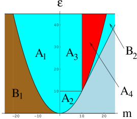
Figure 5: Phase diagram in the space of $\varepsilon$ and $m$: the classically allowed regions defined by the conditions in Table 3 for the different orbits. Here $s=5$ and ${\rm sgn}(eB)=-1$.

This phase diagram should be compared with Fig. 3, the plot of the energy levels from the quantum mechanical calculation. In this way, the different exact levels can be classified in terms of the corresponding classical orbits. We should stress again that these orbits are not necessarily periodic. Examples will be shown in Sec. IV.

IV Comparison of the current distributions and the classical trajectories

An apparent correspondence between the classical orbits and the quantum states can also be made by calculating the current flow patterns in the magnetic anti-dot system. The particle (probability) current density Lent:cikk ; Schwabl:book in magnetic field is given by

$${\bf j}=\frac{i\hbar}{2M}\left(\Psi\,{\rm grad}\Psi^{*}-\Psi^{*}{\rm grad}\Psi\right)-\frac{e}{M}\,{\bf A}{|\Psi|}^{2}.$$ (31)

Using the vector potential (2) the current density (in our units) for states $\Psi_{m,n}$ can be written as ${\bf j}=j_{\varphi}\,\frac{\hat{{\bf e}}_{\varphi}}{r}$, where

$$j_{\varphi}(\tau)=\frac{\hbar}{2M}\,{|\Psi_{m,n}|}^{2}\left[2m-{\rm sgn}(eB)\left(\tau^{2}-\tau_{\rm R}^{2}\right)\Theta\left(\tau-\tau_{\rm R}\right)\right],$$ (32)

and $\hat{{\bf e}}_{\varphi}$ is the unit vector in the $\varphi$ direction.

Solving the secular equation (9) and then determining the normalized eigenstates, the related current densities can be calculated from (32). Figures 6-8, 10 and 11 show the current flow patterns for given eigenstates and the corresponding classical trajectories of the particle. The missing flux quanta is $s=5$ and ${\rm sgn}(eB)=-1$ in all figures. In these figures the current density ${\bf j}({\bf r})$ at point ${\bf r}$ is represented by an arrow with length proportional to the magnitude of the current density and the midpoint of the arrow is at the point ${\bf r}$. At a given energy and quantum number $m$ corresponding to the classical canonical momentum $p_{\varphi}=\hbar m$ the cyclotron radius and the guiding center of the classical orbit is calculated from Eq. (17). Hence the classical trajectory of the particle can be determined and are shown in the figures (scaling is in units of the magnetic length $l$). In Figs. 9 and 12 the radial dependence of the current density is plotted for the corresponding eigenstates. States $(m,n)=(-1,0),(0,0)$ and $(1,0)$ were called magnetic edge states in Ref. Sim:cikk, .

In Fig. 6 the current inside the non-magnetic region flows clockwise (the magnitude of the current density is negative in accordance with Fig. 9), while outside the magnetic dot it flows counterclockwise. The classical trajectories inside the dot form a ‘caustic’ and the current is enhanced here in the clockwise direction. From Table 3 we find that the orbit is of type $A_{1}$. The trajectory apparently also satisfies the conditions given in Table 2 (without the requirement for the periodicity of the orbits).

In Fig. 7 for state $m=0$ and $n=0$ the current is zero inside the magnetic dot. This can easily be seen from Eq. (32), while the direction of the current flow is counterclockwise outside. The orbit is a limiting case between types $A_{1}$ and $A_{2}$. Figure 8 for state $m=1$ and $n=0$ shows a counterclockwise current flow both inside and outside the magnetic dot. The current $j_{\varphi}$ is positive everywhere as it can be also seen in Fig. 9. The orbit is again of type $A_{2}$, in accordance with the conditions given in Tables 2 and 3.

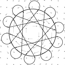
Figure 6: The current flow (in units of $\hbar/(2M)$) for state $m=-1$ and $n=0$. The classical orbit is of type $A_{1}$. Here and in Figs. 9-12 the missing flux quanta is $s=5$, and we choose ${\rm sgn}(eB)=-1$.

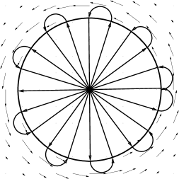
Figure 7: The current flow (in units of $\hbar/(2M)$) for state $m=0$ and $n=0$. The classical orbit is of type $A_{2}$.

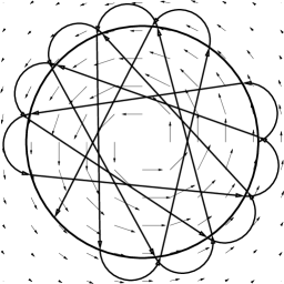
Figure 8: The current flow (in units of $\hbar/(2M)$) for state $m=1$ and $n=0$. The classical orbit is of type $A_{2}$.

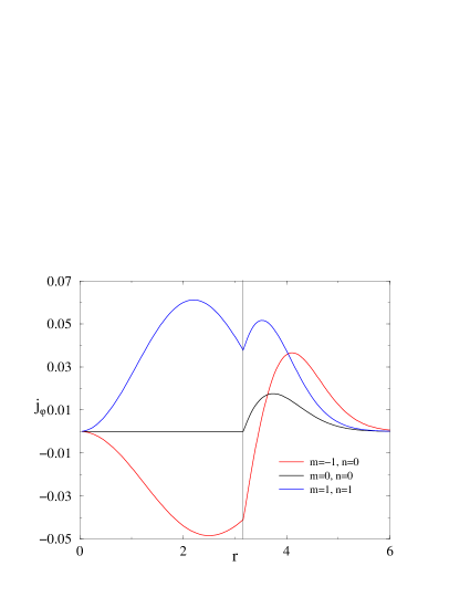
Figure 9: The current densities $j_{\varphi}$ as functions of $r$ (in units of $l$) for states shown in Figs. 6-8. The vertical line is at $r=R$.

One can observe that the current density $j_{\varphi}$ is not differentiable at $r=R$. This is because the theta function in Eq. (32). Physically, this is a consequence of the step function behaviour of the magnetic field. Nevertheless, the divergence of the current density vector ${\bf j}$ is still zero everywhere.

Finally, orbits of types $A_{3}$ and $A_{4}$ are shown in Figs. 10 and 11 for states $(m,n)=(1,6)$ and $(14,2)$, respectively. Similarly, for these states the corresponding current densities as functions of the distance from the origin are plotted in Fig. 12.

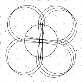
Figure 10: The current flow (in units of $\hbar/(2M)$) for state $m=1$ and $n=6$. The classical orbit is of type $A_{3}$.

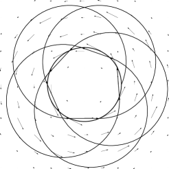
Figure 11: The current flow (in units of $\hbar/(2M)$) for state $m=14$ and $n=2$. The classical orbit is of type $A_{4}$.

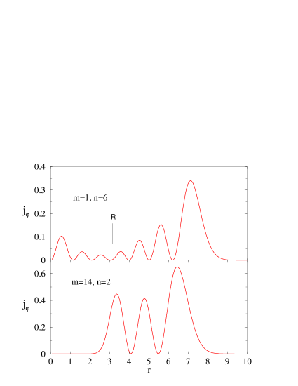
Figure 12: The current densities $j_{\varphi}$ as functions of $r$ (in units of $l$) for states shown in Figs. 10-11. The parameters are the same as in Fig. 6. The vertical line is at $r=R$.

For both states the current is very small inside the magnetic dot. In the case of state $(m,n)=(1,6)$, the trajectories almost cross the origin ($m$ is small), while for state $(m,n)=(14,2)$ only a small portion of the trajectory penetrates into the magnetic anti-dot regions. The qualitative agreement between the current flow patterns and the classical trajectories is, again, clearly visible.

Note that in all of these figures the classical trajectories are not periodic orbits with energy corresponding to the given eigenstate. This is not surprising, since the quantization should not be applied to periodic orbits in real space but to the motion on the two-dimensional torus parametrized by the action variables and their canonically conjugate angle variables (for details see, eg, Ref. Brack:book, ). In fact, the Berry-Tabor formula (11) suggests that an infinite number of periodic orbits with proper weights can only result in the correct quantum mechanical density of states.

It has been shown by Halperin Halperin:cikk that the probability current can be related to the derivative of the energy levels with respect to the angular momentum quantum number:

$$I_{m,n}=\int_{0}^{\infty}\,{\bf j}\,{\bf\hat{e}}_{\varphi}\,dr=\frac{1}{h}\,\frac{\partial E_{m,n}}{\partial m}.$$ (33)

In Fig. 13 the integral of the current densities given in Eq. (33) is plotted as functions of $m$ for $n=0,1,2$. One can see that for $m\ll 0$ the total current is zero (these are the orbits of type $B_{1}$ in our classification) and that for $m\gg 2s$ it tends to a constant value (type $B_{2}$). The current is negative for states corresponding to orbits of type $A_{1}$, while it increases monotonically for states corresponding to orbits of types $A_{2}-A_{4}$.

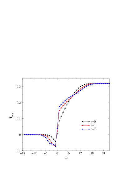
Figure 13: The total current $I_{m,n}$ (in units of $\hbar/(2M)$) obtained from the integral of $j_{\varphi}$ given in (33) as functions of $m$ for $n=0,1,2$. The parameters are the same as in Fig. 6.

This is in accordance with the right hand side of Eq. (33) using the energy dispersion (the $m$ dependence of the energy levels) plotted in Fig. 3.

V Conclusions

In this paper we investigated the energy spectrum of the circular magnetic anti-dot systems obtained from exact quantum and semiclassical calculations. In the proper dimensionless variables the only relevant parameter of the system is the missing flux quantum. The system is separable, and in the quantum calculation the energy levels are the solutions of the secular equation derived from the matching conditions of the wave functions inside and outside the dot. In the semiclassical treatment we presented two different methods. On the one hand, the density of states was calculated using the Berry-Tabor formula. On the other hand, the energy levels obtained from the Bohr-Sommerfeld quantization rules. The main difference between the two methods is that in the first case one needs to characterize the possible periodic orbits in real space, while in the latter, the motion of the particle is on a torus in the space of the action variables. In our numerical results we compared the quantum energy spectrum and that obtained in the semiclassical approach. We showed that the energy levels of the magnetic anti-dot systems obtained from the two semiclassical methods were in good agreement with the numerically exact quantum results for weak magnetic fields. However, by increasing the magnetic field, a slight deviation between the exact and the semiclassically approximated energy levels can be observed. We argued that the reason for this discrepancy may be traced back to the fact that the Maslov index should be magnetic field dependent. A thorough investigation of this problem might be an interesting future work.

A classification of the energy spectrum for arbitrary magnetic fields was presented in terms of the classical orbits defined by their cyclotron radius and guiding center. Such identifications are based on the explicit relations between these classical parameters of the orbits and the quantum states. The correspondence between the quantum states and the classical trajectories can be made transparent by drawing a phase diagram with regions corresponding to six different types of orbits in the space of energy and angular momentum quantum number.

Finally, we calculated the current flow patterns for eigenstates that correspond to orbits with trajectories penetrating into the field-free region. The related classical trajectories were also shown for the sake of comparisson. From these results one can see the close correspondence between the structure of the trajectories and the distribution of the current densities obtained from the quantum calculations.

From the energy spectrum of the magnetic anti-dot systems one can determine the free energy. The good agreement between the semiclassical and quantum treatment of the system allows us to use semiclassical methods in the weak field limit for calculating the energy spectrum. Therefore, the semiclassical approach provides a useful starting point for successive studies of thermodynamic properties, such as magnetization. Moreover, the semiclassical approximation can be an effective tool for investigating arbitrarily shaped magnetic anti-dots (which would be a very difficult task in the quantum case) or systems with more complicated magnetic field profiles.

Appendix A The Berry-Tabor formula

The quantized energies can be recovered if we express the Hamiltonian in terms of $I_{i}$

$$E(n_{1},n_{2},...,n_{d})=H(I_{1},I_{2},...,I_{d})=$$

$$H\left(\hbar\left(n_{1}+\nu_{1}/4\right),\hbar\left(n_{2}+\nu_{2}/4\right),...,\hbar\left(n_{d}+\nu_{d}/4\right)\right).$$

The semiclassical density of states is the density of these energies:

$$d(E)=\sum_{n_{1},n_{2},...,n_{d}=0}^{\infty}\delta\left(E-E(n_{1},n_{2},...,n_{d})\right).$$ (35)

The density of states can be rewritten via the Poisson resummation technique

$$d(E) = \int d^{d}I\delta(E-H(I_{1},I_{2},...,I_{d}))\times$$ (36)

$$\prod_{i=1}^{d}\sum_{n_{i}=-\infty}^{+\infty}\delta(I_{i}-\hbar(n_{i}+\nu_{i}/4))=$$

$$\sum_{m_{1},m_{2},...,m_{d}=-\infty}^{\infty}\int\frac{d^{d}Idt}{2\pi\hbar^{d+1}}\times$$

$$e^{\frac{i}{\hbar}(t(E-H(I_{1},...,I_{d}))+2\pi\sum_{i}m_{i}(I_{i}-\hbar\nu_{i}/4))}.$$

Here, we used the Fourier expansion of the delta spike train. The term $m_{i}=0\;(i=1,2,...,d)$ can be evaluated directly and yields the non-oscillatory average density of states. Other terms can be evaluated by the saddle point method, when $\hbar\rightarrow 0$. The saddlepoint conditions select the periodic orbits of the system, and the result of the integration is

$$d(E) = d_{0}(E)+\sum_{p}\sum_{j=1}^{+\infty}\frac{(2\pi)^{(d-1)/2}}{2^{(\chi_{p}-1)}\hbar^{(d+1)/2}}\times$$ (37)

$$\frac{\cos\left({jS_{p}(E)/\hbar}-\frac{\pi}{2}j\nu_{p}+\frac{\pi}{4}(d-1)\right)}{\sqrt{(jT_{p})^{d-1}(-\det{\bf D}_{p})}}.$$

Here $p$ is the index of the primitive periodic orbits, $j$ is the number of repetitions, $S_{p}$ is the classical action along the orbit, $T_{p}$ is the time period of the orbit, and $\nu_{p}$ is the Maslov index. The quantity $\chi_{p}$ is the number of action variables of the periodic orbit whose saddle point value is zero $(I_{k}=0)$, since in this case the Gaussian saddle point integral is only one-sided, and its contribution is $1/2$ of the full Gaussian integral. The matrix ${\bf D}_{p}$ is related to the second derivative matrix

$$\det{\bf D}=\det\left(\begin{array}[]{cc}\frac{\partial^{2}H(I_{1},...,I_{d})}{\partial I_{i}\partial I_{j}}&\frac{\partial H(I_{1},...,I_{d})}{\partial I_{i}}\\ \frac{\partial H(I_{1},...,I_{d})}{\partial I_{j}}&0\\ \end{array}\right).$$ (38)

Equation (37) is the generic form of the semiclassical density of states in terms of periodic orbits, known as the Berry-Tabor formula Berry-Tabor:cikk .

In two dimensions, very often the Hamiltonian cannot be expressed with the action variables explicitly, only the implicit function

$$I_{2}=g(I_{1},H),$$ (39)

is available. In this case it is more useful to express the quantities in the Berry-Tabor trace formula in terms of the derivatives of $g$. Taking the partial derivative of (39) with respect to $I_{1}$ yields

$$0=\frac{\partial g(I_{1},H)}{\partial I_{1}}+\frac{\partial g(I_{1},H)}{\partial H}\frac{\partial H(I_{1},I_{2})}{\partial I_{1}},$$ (40)

while the partial derivative of (39) with respect to $I_{2}$ gives

$$1=\frac{\partial g(I_{1},H)}{\partial H}\frac{\partial H(I_{1},I_{2})}{\partial I_{2}}.$$ (41)

The frequencies can be expressed from these equations as

$$\omega_{1} = \frac{\partial H(I_{1},I_{2})}{\partial I_{1}}=-\frac{\frac{\partial g(I_{1},H)}{\partial I_{1}}}{\frac{\partial g(I_{1},H)}{\partial H}},$$ (42)

$$\omega_{2} = \frac{\partial H(I_{1},I_{2})}{\partial I_{2}}=\frac{1}{\frac{\partial g(I_{1},H)}{\partial H}}.$$ (43)

Periodic orbits are recovered from $\omega_{1}=\frac{2\pi n_{1}}{T}$ and $\omega_{2}=\frac{2\pi n_{2}}{T}$. The action $I_{1}$ for a periodic orbit at energy $E$ can be obtained by solving equation

$$\frac{\omega_{1}}{\omega_{2}}=\frac{n_{1}}{n_{2}}=\frac{n_{1,p}}{n_{2,p}}=-\frac{\partial g(I_{1},E)}{\partial I_{1}},$$ (44)

where we introduced $n_{1}=jn_{1,p}$ and $n_{2}=jn_{2,p}$ corresponding to the primitive orbit. Then the period can be expressed simply as

$$T=2\pi n_{2,p}\frac{\partial g(I_{1},H)}{\partial H}.$$ (45)

The main determinant to be calculated reads

$$\det{\bf D} = \left|\begin{array}[]{ccc}\frac{\partial^{2}H(I_{1},I_{2})}{\partial I_{1}^{2}}&\frac{\partial^{2}H(I_{1},I_{2})}{\partial I_{1}\partial I_{2}}&\frac{\partial H(I_{1},I_{2})}{\partial I_{1}}\\ \frac{\partial^{2}H(I_{1},I_{2})}{\partial I_{1}\partial I_{2}}&\frac{\partial^{2}H(I_{1},I_{2})}{\partial I_{2}^{2}}&\frac{\partial H(I_{1},I_{2})}{\partial I_{2}}\\ \frac{\partial H(I_{1},I_{2})}{\partial I_{1}}&\frac{\partial H(I_{1},I_{2})}{\partial I_{2}}&0\\ \end{array}\right|=$$ (50)

$$= \left(-\frac{\partial^{2}H}{\partial I_{1}^{2}}\left(\frac{\partial H}{\partial I_{2}}\right)^{2}+2\frac{\partial^{2}H}{\partial I_{1}\partial I_{2}}\frac{\partial H}{\partial I_{1}}\frac{\partial H}{\partial I_{2}}\right.$$

$$\left.-\frac{\partial^{2}H}{\partial I_{2}^{2}}\left(\frac{\partial H}{\partial I_{1}}\right)^{2}\right).$$

Now, the second derivatives of $H$ can be expressed with the second derivatives of $g$ by taking further partial derivatives of (40) and (41) with respect to $I_{1}$ and $I_{2}$. Then we can express the second derivatives as

$$\frac{\partial^{2}H}{\partial I_{1}^{2}} = \frac{1}{\left(\frac{\partial g}{\partial H}\right)^{3}}\left(2\frac{\partial^{2}g}{\partial H\partial I_{1}}\frac{\partial g}{\partial I_{1}}\frac{\partial g}{\partial H}-\frac{\partial^{2}g}{\partial H^{2}}\left(\frac{\partial g}{\partial I_{1}}\right)^{2}\right.$$ (51)

$$\left.-\frac{\partial^{2}g}{\partial I_{1}^{2}}\left(\frac{\partial g}{\partial H}\right)^{2}\right),$$

$$\frac{\partial^{2}H}{\partial I_{1}\partial I_{2}} = \frac{1}{\left(\frac{\partial g}{\partial H}\right)^{3}}\left(\frac{\partial^{2}g}{\partial H^{2}}\frac{\partial g}{\partial I_{1}}-\frac{\partial^{2}g}{\partial I_{1}\partial H}\frac{\partial g}{\partial H}\right),$$ (52)

$$\frac{\partial^{2}H}{\partial I_{2}^{2}} = -\frac{1}{\left(\frac{\partial g}{\partial H}\right)^{3}}\frac{\partial^{2}g}{\partial H^{2}}.$$ (53)

Using these expressions, the determinant becomes

$$\det{\bf D}=-\frac{1}{\left(\frac{\partial g}{\partial H}\right)^{3}}\frac{\partial^{2}g}{\partial I_{1}^{2}}=-\frac{(2\pi n_{2,p})^{3}}{T^{3}}\frac{\partial^{2}g}{\partial I_{1}^{2}}.$$ (54)

The density of states in two dimensions is then

$$d(E)=d_{0}(E)+$$

$$\sum_{p}\sum_{j=1}^{+\infty}\frac{\cos\left({jS_{p}(E)/\hbar}-\frac{\pi}{2}j\nu_{p}+\frac{\pi}{4}(d-1)\right)}{2^{\chi_{p}}\pi(\hbar)^{3/2}\sqrt{j(n_{2,p})^{3}\frac{\partial^{2}g}{\partial I_{1}^{2}}/T_{p}^{2}}}.$$ (55)

Appendix B Derivation of the cyclotron radius and the guiding center

The cyclotron radius can be determined from the energy $E$ of the particle. The energy is conserved, and obviously $E=\frac{1}{2}\,M\omega_{c}^{2}\,\varrho^{2}$, thus

$$\frac{\varrho}{l}=\sqrt{\varepsilon}.$$ (56)

The guiding center may be calculated as follows. As we have seen, the conjugate momentum given by Eq. (15) is a constant of motion, therefore, e.g., for $r>R$ the right hand side of (15) should also be a constant at any point of the orbit. At first apply this equation for points $P$ and $Q$, which are the points closest to and farthest from the origin (the center of the circle of radius $R$) of an orbit lying outside the anti-dot. These are special points of the orbits for which the right hand side of Eq. (15) has a simpler form. Then the distances of points $P$ and $Q$ from the origin are $r_{P}=c-\varrho$ and $r_{Q}=c+\varrho$ (we assume that point $Q$ is farther from the origin). From a simple geometrical argument one finds that the angular velocity at points $P$ and $Q$ satisfies the following equations

$$r_{P}\,\dot{\varphi}_{P} = \varrho\,\omega_{c}\,{\rm sgn}(eB),$$ (57)

$$r_{Q}\,\dot{\varphi}_{Q} = -\varrho\,\omega_{c}\,{\rm sgn}(eB).$$ (58)

Substituting, for example, $r_{P}=c-\varrho$ and $\dot{\varphi_{P}}$ from (57) into Eq. (15), and using (56), we find

$$\frac{c}{l}=\sqrt{\varepsilon+2\,m_{\rm eff}}.$$ (59)

The same results can be obtained by using (58) for point $Q$. If the oribit encompasses the anti-dot then the right hand side of (57) should be multiplied by a factor of $-1$. The case of orbits with trajectories penetrating into the anti-dot can be treated similarly. However, the expressions for the cyclotron radius and the guiding center are the same as above for all cases.

Appendix C Contribution of the cyclotron orbits to the semiclassical density of states

In the case of the cyclotron orbits, the integral in $I_{\varphi}$ in Eq. (36) has to be calculated directly rather than using the saddlepoint method. As $I_{\varphi}$ is constant, the integrand does not depend on the integration variable and therefore the integral is equal to the measure of the interval of the possible $I_{\varphi}$s. Without loss of generality, we take $\rm{sgn}(eB)=-1$ in this section.

C.1 Cyclotron orbits of type $B_{1}$

Cyclotron orbits which do not encompass the anti-dot (type $B_{1}$) are possible at any value of $\rho$ and any negative angular momentum $p_{\varphi}$ (see Table 3). At point $P$ of these orbits (points $P$ and $Q$ of a cyclotron orbit are defined in Appendix B), from Eqs. (14) and (15) we obtain

$$I_{\varphi}=p_{\varphi}=Mr_{P}^{2}\dot{\varphi}_{P}+eB\frac{r_{P}^{2}-R^{2}}{2}.$$ (60)

This is minimal when $r_{P}=R$ (and the cyclotron orbit touches the boundary of the anti-dot), and is maximal when the orbit is placed as far as possible from the anti-dot. By denoting the radius of the system with ${\cal L}$ (in units of $l$) the intergation in (36) with respect to $I_{\varphi}$ yields a factor $\Delta I_{\varphi}=I_{\varphi}(R)-I_{\varphi}({\cal L})$. Using (60) and (57), one finds

$$\frac{\Delta I_{\varphi}}{\hbar}={\cal L}\sqrt{\varepsilon}-\sqrt{2s\varepsilon}+\frac{1}{2}({\cal L}^{2}-2s).$$ (61)

The $I_{r}$- and $t$-integrals can be evaluated with the saddle point method, just as in the case of a one-dimensional system. The determinant of the second derivative matrix is

$${\det}\bf D=\det\begin{pmatrix}-\frac{\partial^{2}H}{{\partial}I_{r}^{2}}T&-\frac{{\partial}H}{{\partial}I_{r}}\cr-\frac{{\partial}H}{{\partial}I_{r}}&0\end{pmatrix}=-\left(\frac{{\partial}H}{{\partial}I_{r}}\right)^{2}.$$ (62)

From Eqs. (41) and (23), we find

$$\frac{{\partial}H}{{\partial}I_{r}} = \frac{1}{\frac{{\partial}g}{{\partial}E}}=\omega_{c},$$ (63)

$$\det\bf D = -\omega_{c}^{2}.$$ (64)

Thus, the total amplitude of these orbits in the periodic orbit sum is

$$A_{c}^{-} \equiv \frac{\Delta I_{\varphi}}{\hbar}\,\frac{1}{\hbar\omega_{c}}$$ (65)

$$= \frac{1}{\hbar\omega_{c}}\left[{\cal L}\sqrt{\varepsilon}-\sqrt{2s\varepsilon}+\frac{1}{2}({\cal L}^{2}-2s)\right].$$

The action can be calculated from Eq. (23), and for $p_{\varphi}/\hbar\equiv m<0$ we have

$$S=2\pi I_{r}=\hbar\pi\varepsilon,$$ (66)

and their Maslov index is $\mu=2$, therefore the contribution to the semiclassical level density from these orbits reads

$$d_{c}^{-}(E)=A_{c}^{-}\sum_{j=1}^{\infty}\cos\left(j\varepsilon\pi-j\pi\right).$$ (67)

The sum has Dirac delta peaks at $\varepsilon=2n+1$, where $n=0,1,2,\ldots$ and $m<0$. These are the familiar Landau levels of an electron for $m<0$.

C.2 Cycltoron orbits of type $B_{2}$

For cyclotron orbits encompassing the anti-dot (type $B_{2}$) the angular momentum satisfies the condition $p_{\varphi}/\hbar=m>2s$ (see Table 3). At point $Q$ of these orbits, using (14) and (15), we can write

$$I_{\varphi}=p_{\varphi}=Mr_{Q}^{2}\dot{\varphi_{Q}}+eB\frac{r_{Q}^{2}-R^{2}}{2}.$$ (68)

The minimum and the maximum of $r_{Q}$ are $\varrho$ and $2\varrho-R$, respectively. Between these values, $I_{\varphi}$, as a function of $r_{Q}$, is monotonic, thus the integration in (36) over $I_{\varphi}$ gives $\Delta I_{\varphi}=I_{\varphi}(\varrho)-I_{\varphi}(2\varrho-R)$. Using (68) and (58), we have

$$\frac{\Delta I_{\varphi}}{\hbar}=\frac{\varepsilon}{2}+s-\sqrt{2s\varepsilon}.$$ (69)

Similarly to (65), the amplitude of the orbits becomes

$$A_{c}^{+}\equiv\frac{\Delta I_{\varphi}}{\hbar}\,\frac{1}{\hbar\omega_{c}}=\frac{\frac{\varepsilon}{2}+s-\sqrt{2s\varepsilon}}{\hbar\omega_{c}}.$$ (70)

Using (23), the action for $p_{\varphi}/\hbar\equiv m>2s$ is

$$S=2\pi I_{r}=\hbar\pi\left(\varepsilon+2s-2m\right),$$ (71)

Finally, the contribution to the periodic orbit sum of these orbits is

$$d_{c}^{+}(E) = \!\!A_{c}^{+}\sum_{j=1}^{\infty}\cos\left[\pi j(\varepsilon+2s-2m)-j\pi\right].$$ (72)

The sum has Dirac delta peaks at $\varepsilon=2(m-s)+2n+1$, where $m$ and $n$ are non-negative integers, and $m>2s$. These are again the familiar Landau levels of an electron for $m>2s$.

References

- (1) C. W. J. Beenakker and H. van Houten, Solid State Phys. 44, 1 (1991).
- (2) C. L. Foden, M. L. Leadbeater, J. H. Burroughes, and M. Pepper, J. Phys.: Condens. Matter 6, L127 (1994).
- (3) M. L. Leadbeater et al., Phys. Rev. B 52, R8629 (1995).
- (4) M. L. Leadbeater et al., J. Appl. Phys. 69, 4689 (1991).
- (5) K. M. Krishnan, Appl. Phys. Lett. 61, 2365 (1992).
- (6) A. Nogaret, S. J. Bending, and M. Henini, Phys. Rev. Lett. 84, 2231 (2000).
- (7) D. N. Lawton, A. Nogaret, S. J. Bending, D. K. Maude, J. C. Portal, and M. Henini, Phys. Rev. B 64, 033312 (2001).
- (8) A. Nogaret, D. N. Lawton, D. K. Maude, J. C. Portal, and M. Henini, Phys. Rev. B 67, 165317 (2003).
- (9) D. Uzur, A. Nogaret, H. E. Beere, D. A. Ritchie, C. H. Marrows, and B. J. Hickey, Phys. Rev. B 69, 241301 (2004).
- (10) A. Smith, R. Taboryski, L. T. Hansen, C. B. Sørensen, P. Hedegård, and P. E. Lindelof, Phys. Rev. B 50, 14726 (1994).
- (11) A. K. Geim et al., Nature (London) 390, 259 (1997).
- (12) J. E. Müller, Phys. Rev. Lett. 68, 385 (1992).
- (13) D. V. Khveshchenko and S. V. Meshkov, Phys. Rev. B. 47, 12051 (1993).
- (14) Götz J. O. Schmidt, Phys. Rev. B. 47, 13007 (1993).
- (15) F. M. Peeters and P. Vasilopoulos, Phys. Rev. B 47, 1466 (1993).
- (16) M. Calvo, Phys. Rev. B 48, 2365 (1993).
- (17) F. M. Peeters and A. Matulis, Phys. Rev. B 48, 15166 (1993).
- (18) P. Schmelcher and D. L. Shepelyansky, Phys. Rev. B 49, 7418 (1994).
- (19) A. Matulis, F. M. Peeters and P. Vasilopoulos, Phys. Rev. Lett. 72, 1518 (1994).
- (20) M. Nielsen and P. Hedegård, Phys. Rev. B 51, 7679 (1995).
- (21) I. S. Ibrahim and F. M. Peeters, Phys. Rev. B 52, 17321 (1995).
- (22) H.-S. Sim, K.-H. Ahn, K. J. Chang, G. Ihm, N. Kim, and S. J. Lee, Phys. Rev. Lett. 80, 1501 (1998).
- (23) D. Urbach, Dynamique Classique d’un Électron dans un Champ Magnétique Périodique, Thesis, 1998, Lausanne, Switzerland.
- (24) N. Kim, G. Ihm, H.-S. Sim, and K. J. Chang, Phys. Rev. B 60, 8767 (1999).
- (25) M. Governale and D. Boese, Appl. Phys. Lett. 77, 3215 (2000).
- (26) N. Kim, G. Ihm, H.-S. Sim, and T. W. Kang, Phys. Rev. B 63, 235317 (2001).
- (27) H.-S. Sim, G. Ihm, N. Kim, K. J. Chang, Phys. Rev. Lett. 87, 146601 (2001).
- (28) S. M. Badalyan and F. M. Peeters, Phys. Rev. B 64, 155303 (2001).
- (29) J. Reijniers, F. M. Peeters, and A. Matulis, Phys. Rev. B 64, 245314 (2001).
- (30) D. Frustaglia, M. Hentschel, and K. Richter, Phys. Rev. Lett. 87, 256602 (2001).
- (31) Z. Vörös, T. Tasnádi, J. Cserti, and P. Pollner, Phys. Rev. E 67, 065202 (2003).
- (32) L. Solimany and B. Kramer, Solid State Comm. 96, 471 (1995).
- (33) G. Wentzel, Z. Phys. 38, 58 (1926); H. A. Kramers, ibid. 39, 828 (1926); M. L. Brillouin, Phys. Radium 6, 353 (1926).
- (34) J. B. Keller, Ann. Phys. (Leipzig) 4, 180 (1958); J. B. Keller and S. I. Rubinov, ibid. 9, 24 (1960).
- (35) M. V. Berry and M. Tabor, Proc. Roy. Soc. London Ser. A 349, 101 (1976); ibid. 356, 375 (1977); M. V. Berry and M. Tabor, J. Phys. A 10, 371 (1977).
- (36) R. Balian and C. Bloch, Ann. Phys. (N.Y.) 69, 76 (1972); ibid. 85, 514 (1974).
- (37) M. C. Gutzwiller, J. Math. Phys. (N.Y.) 11, 1791 (1970); ibid. 12, 343 (1971).
- (38) V. M. Strutinsky, Nukleonik 20, 679 (1975); V. M. Strutinsky and A. G. Magner, Fiz. Elem. Chastits At. Yadra 7, 356 (1976). [Sov. J. Part. Nucl. 7, 138 (1976)].
- (39) S. C. Creagh and R. G. Littlejohn, Phys. Rev. A 44, 836 (1990); J. Phys. A 25, 1643 (1991).
- (40) M. Brack and R. K. Bhaduri, Semiclassical Physics, (Addison-Wesley, Reading MA, 1997).
- (41) J. Blaschke and M. Brack, Phys. Rev. A 56, 182 (1997).
- (42) K. Hornberger and U. Smilansky, Physics Reports 367, 249 (2002); K. Hornberger, Spectral Properties of Magnetic Edge States, Thesis, 2001, München, Germany.
- (43) S. Klama, J. Phys.: Condens. Matter 5, 5609 (1993).
- (44) L. A. Falkovsky and S. Klama, J. Phys.: Condens. Matter 5, 4491 (1993).
- (45) C. S. Lent, Phys. Rev. B 43, 4179 (1991).
- (46) B. I. Halperin, Phys. Rev. B 25, 2185 (1982).
- (47) A. Abramowitz and I. A. Stegun, Handbook of Mathematical Functions (Dover Publication, New York, 1972).
- (48) J. Cserti, P. Polinák, G. Palla, U. Zülicke, and C. J. Lambert, Phys. Rev. B 69, 134514 (2004).
- (49) F. Schwabl, Quantum Mechanics (Springer-Verlag, Berlin, 1990).