Spin current and polarization in impure 2D electron systems with spin-orbit coupling

Abstract

We derive the transport equations for two-dimensional electron systems with spin-orbit interaction and short-range spin-independent disorder. In the limit of slow spatial variations of the electron distribution we obtain coupled diffusion equations for the electron density and spin. Using these equations we calculate electric-field induced spin accumulation and spin current in a finite-size sample for arbitrary ratio between spin-orbit energy splitting $\Delta$ and elastic scattering rate $\tau^{-1}$. We demonstrate that the spin-Hall conductivity vanishes in an infinite system independent of this ratio.

Introduction. The subject of the novel and quickly developing field of spintronics is the transport of electronic spins in low-dimensional and nanoscale systems. A possibility of coherent spin manipulation represents an ultimate goal of this field. Typically, spin transport is strongly affected by a coupling of spin and orbital degrees of freedom. The influence of the spin-orbit interaction is two-fold. The momentum relaxation due to diffusive scattering of carriers, e.g. by disorder, inevitably leads to a spin relaxation and destroys spin coherence. On the other hand, the controlled orbital motion of carriers can result in a coherent motion of their spins. Thus, spin-orbit coupling is envisaged as a possible tool for spin control in electronic devices. In particular, it is possible to generate spin polarization and spin currents by applying electric field, the phenomenon known as the spin-Hall effect.

Although the study of spin-Hall effect recently evolved into a subject of intense research MNZ ; SCN ; CSS ; SL ; HBW ; Sh ; SHT ; R ; IBM ; XX ; BNM ; D , the issue remains highly controversial. Sinova et al. SCN have predicted that in a clean, infinite, homogeneous 2DES the spin-current $\hat{j}^{i}_{k}=\frac{1}{4}\{\hat{\sigma}_{i},\hat{v}_{k}\}$ develops a non-zero expectation value under an external electric field ${\bf E}$. (Here $\frac{1}{2}\hat{\bm{\sigma}}$ and $\hat{\bf v}$ are the operators of the electron spin and velocity, respectively.) The spin-Hall conductivity, defined as the ratio $\sigma_{sH}=-j^{z}_{y}/E_{x}$, was predicted to have a universal value $\sigma_{sH}=\frac{e}{8\pi}$, independent of the magnitude of the spin-orbit energy splitting $\Delta$. The effect of impurity scattering on a spin current has been discussed in Refs. SL ; IBM ; BNM ; XX . Schliemann and Loss SL and Burkov et al. BNM found that the spin-Hall conductivity disappears in the dirty limit $\Delta\ll\tau^{-1}$, reaching the universal value only for sufficiently clean regime, $\Delta\gg\tau^{-1}$. The clean regime has been analyzed by Inoue et al. IBM , who argued that the spin-current completely disappears due to vertex corrections. Recently, Dimitrova D obtained the universal value independent of the relation between the spin-orbit splitting $\Delta$ and the impurity scattering rate.

Because the spin-current is not measurable directly, its physical meaning is obscure. In the presence of spin-orbit interaction, electron spin is not a conserved quantity, and a spin current is not directly related to the transport of spins. In particular, Rashba R demonstrated that spin current can be non-zero even in equilibrium, as the symmetry of an isotropic spin-orbit Hamiltonian allows non-zero in-plane currents $j^{x}_{y}=-j^{y}_{x}\neq 0$. A more meaningful quantity is spin polarization (spin accumulation) rather than a spin current. Equilibrium currents do not lead to spin-accumulation. It remains unclear whether the predicted nonequilibrium spin-Hall currents $j^{z}_{y}$ accumulate near sample boundaries. Bulk polarization has been studied in both the three-dimensional LNE and two-dimensional E electron systems in the electric field.

In this Letter, we develop a consistent microscopic approach to spin transport in impure 2DES. We derive a quantum kinetic equation which describes the evolution of a density matrix of a non-interacting 2DES. For length scales exceeding the mean free path, this equation reduces to a modified diffusion equation. We then compute spin polarization and spin current in a general situation when the finite-size system is driven out of equilibrium by an external electric field as well as by the density gradient. We find that the spin current actually vanishes in an infinite system for arbitrary $\Delta\tau$.

However, in a mesoscopic conductor connected to two massive metallic contacts, non-equilibrium spin currents $j^{z}_{y}$ flow in the vicinity of the contacts (as shown in Fig. 1). A non-zero spin-Hall effect can also be achieved in an infinite system by applying a finite frequency electric field. We evaluate the ac spin-Hall conductivity, which is maximal for a frequency of order of the spin relaxation rate. This result is instructive for making a connection with previous works and clarifying the ’universality’ issue of the spin-Hall conductivity.

Kinetic equation. Non-interacting electrons in an asymmetric quantum well can be described by a single particle Hamiltonian

$$H=\frac{1}{2m}\left({\bf p}-\frac{e{\bf A}(t)}{c}\right)^{2}+\alpha~{}\hat{\bm{\eta}}\cdot\left({\bf p}-\frac{e{\bf A}(t)}{c}\right)+U_{i},$$ (1)

where ${\bf p}=-i\hbar{\bm{\nabla}}$ is electron momentum, $m$ is the effective mass, ${\bf A}(t)$ is a vector potential of the uniform electric field ${\bf E}=-{\bf\dot{A}}/c$, and $\hat{\bm{\eta}}$ is proportional to the electron spin operator. (We neglect terms qubic in ${\bf p}$.) The disorder potential $U_{i}$ is assumed to be random, short-range, and spin-independent. For the isotropic (“Rashba”) spin-orbit interaction BR , $\hat{\bm{\eta}}={\bf z}\times\hat{\bm{\sigma}}$, where $\hat{\bm{\sigma}}$ are the Pauli matrices. To describe a non-equilibrium state of the system, we use the Keldysh approach RS . We introduce the retarded and advanced Green’s functions $G^{R}$ and $G^{A}$, and Keldysh function $G^{K}$ satisfying Dyson’s equation

$$\left(\hat{G}^{-1}_{0}-\underline{\hat{\Sigma}}\right)\underline{\hat{G}}=1,~{}~{}\underline{\hat{G}}=\left(\begin{array}[]{ll}\hat{G}^{R}&\hat{G}^{K}\\ 0&\hat{G}^{A}\end{array}\right)\ .$$ (2)

Here the lower bar denotes a matrix in Keldysh space, $\hat{G}_{0}^{-1}=i\partial_{t}-\hat{H}$, and $\nu=\frac{m}{2\pi}$ is a density of states per spin direction. Neglecting weak-localization effects, one can relate the self-energy $\underline{\hat{\Sigma}}$ to the Green’s function $\underline{\hat{G}}$ by a standard disorder averaging technique AGD ,

$$\underline{\hat{\Sigma}}=\frac{\delta_{\bf xx^{\prime}}}{2\pi\nu\tau}~{}\underline{\hat{G}}({\bf x},{\bf x})\ .$$ (3)

We consider only the limit where $\tau^{-1}$ and $\Delta$ are small compared to the Fermi energy $p^{2}_{F}/2m$. In the absence of electron-electron interactions, functions $\hat{G}^{R}$ and $\hat{G}^{A}$ are independent of the non-equilibrium state of the system. In the Fourier representation, they are given by

$$\hat{G}^{R,A}_{{\bf p}\varepsilon}=\frac{1}{\epsilon-\xi_{p}-\Delta_{p}\,\hat{\eta}_{\bf p}\pm\frac{i}{2\tau}}\ .$$ (4)

Here $\xi_{p}=(p^{2}-p_{F}^{2})/2m$ is the kinetic energy counted from the equilibrium chemical potential, $\Delta_{p}=\alpha p$ is the energy of the spin-orbit splitting, and $\hat{\eta}_{\bf p}=\hat{\bm{\eta}}\cdot{\bf p}/p$ is the projection of the spin operator $\hat{\bm{\eta}}$ onto the direction of the electron momentum. The Keldysh function $\hat{G}^{K}$ satisfies the equation

$$[\hat{G}^{R}]^{-1}\hat{G}^{K}-\hat{G}^{K}[\hat{G}^{A}]^{-1}=\hat{\Sigma}^{K}\hat{G}^{A}-\hat{G}^{R}\hat{\Sigma}^{K}.$$ (5)

It is now customary to apply the Wigner transformation to Eq. (5), i.e. the Fourier transform with respect to the relative time and space arguments,

$$\hat{G}^{K}(t_{+}{\bf x}_{+};t_{-}{\bf x}_{-})=\frac{i}{\pi}\int\frac{d\varepsilon d^{2}p}{(2\pi)^{2}}~{}\hat{g}_{\bf p\varepsilon}(t,{\bf x})$$

$$\times\,e^{i[{\bf p}+e{\bf A}(t)/c]\delta{\bf x}-i\varepsilon\delta t},$$ (6)

here $t_{\pm}=t\pm\delta t$ and ${\bf x}_{\pm}={\bf x}\pm\delta{\bf x}/2$. In the semiclassical approximation, the Wigner transform of the right-hand side of Eq. (5) can be replaced by a product of the Wigner transforms of $\Sigma$ and $G$:

$$\frac{\partial\hat{g}_{\bf p\varepsilon}}{\partial t}+\frac{1}{2}\left\{\frac{{\bf p}}{m}+\alpha{\bm{\eta}},{\widetilde{\nabla}}\hat{g}_{\bf p\varepsilon}\right\}+i\alpha[\hat{\bm{\eta}}\cdot{\bf p},\hat{g}_{\bf p\varepsilon}]=$$ (7)

$$=-\frac{\hat{g}_{\bf p\varepsilon}}{\tau}+\frac{i}{\tau}\left(\hat{G}^{R}_{\bf p\varepsilon}\hat{\rho}_{\epsilon}-\hat{\rho}_{\epsilon}\hat{G}^{A}_{\bf p\varepsilon}\right)\ ,$$

where ${\widetilde{\nabla}}=\nabla+e{\bf E}\,{\partial}_{\varepsilon}$, and

$$\hat{\rho}_{\varepsilon}=\frac{1}{2\pi\nu}\int\frac{d^{2}p}{(2\pi)^{2}}\,\hat{g}_{\bf p\varepsilon}$$ (8)

is the density matrix of electrons with the energy $\varepsilon$. The total number of particles and their total spin can be expressed via $\hat{\rho}_{\varepsilon}$ as follows,

$$N=\text{Tr}\,\nu\!\int\!d\varepsilon\,\hat{\rho}_{\varepsilon},~{}~{}{\bf S}=\frac{1}{2}\,\text{Tr}\,\nu\!\int\!d\varepsilon\,\hat{\bm{\sigma}}\hat{\rho}_{\varepsilon}$$ (9)

In the limit $\tau\to\infty$ the equation (7) reduces to the ballistic equation of Ref. MH, . Note, however, that the function $\hat{g}_{\bf p\epsilon}$ is not a distribution function in the conventional sense, since it depends on both energy and momentum.

A stationary solution to the quantum kinetic equation (7) is of the form $\hat{g}_{\bf p\varepsilon}=A_{\varepsilon}(\hat{G}^{R}_{\bf p\varepsilon}-\hat{G}^{A}_{\bf p\varepsilon})$, where $A_{\varepsilon}$ is an arbitrary scalar function of the electron energy $\varepsilon$. This solution represents the state in which the charge density is uniform, and spin density is zero. In a non-equilibrium state with the characteristic length scales of the spin and charge densities exceeding the electron mean free path $l=v_{F}\tau$, the distribution $\hat{g}_{\bf p\varepsilon}$ relaxes slowly to equilibrium. To describe this relaxation, we derive the equation for the density matrix $\hat{\rho}_{\varepsilon}({\bf r},t)$. It is useful to move small gradient terms to the right hand of the kinetic equation (7), so that its left hand side describes fast relaxation to the local equilibrium distribution:

$$(\partial_{t}+\tau^{-1})\hat{g}_{\bf p\varepsilon}+i\Delta_{p}[\hat{\eta}_{\bf p},\hat{g}_{\bf p\varepsilon}]=\hat{\cal K}_{\bf p\varepsilon}\equiv\hat{\cal K}^{(0)}_{\bf p\varepsilon}+\hat{\cal K}^{(1)}_{\bf p\varepsilon}\ ,$$ (10)

where

$$\hat{\cal K}^{(0)}_{\bf p\varepsilon}[\hat{\rho}_{\varepsilon}] = {i}{\tau}^{-1}[\hat{G}^{R}_{\bf p\varepsilon}\hat{\rho}_{\varepsilon}-\hat{\rho}_{\varepsilon}G^{A}_{\bf p\varepsilon}]$$

$$\hat{\cal K}^{(1)}_{\bf p\varepsilon}[\hat{g}_{\bf p\varepsilon}] = -\frac{1}{2}\left\{\frac{\bf p}{m}+\alpha\hat{\bm{\eta}},\widetilde{\nabla}\hat{g}_{\bf p\varepsilon}\right\}\ .$$ (11)

Small anisotropic deviations from local equilibrium are due to the gradient term $\hat{\cal K}^{(1)}_{\bf p\varepsilon}$ in the kinetic equation which can be treated perturbatively. The solution to Eq. (10) can formally be written (in the Fourier representation with respect to time) as,

$$\hat{g}_{\bf p\varepsilon} =i\frac{(2\Delta_{p}^{2}-\Omega^{2})\hat{\cal K}_{\bf p\varepsilon}+2\Delta^{2}_{p}\hat{\eta}_{\bf p}\hat{\cal K}_{\bf p\varepsilon}\hat{\eta}_{\bf p}-\Omega\Delta_{p}[\hat{\eta}_{\bf p},\hat{\cal K}_{\bf p\varepsilon}]}{\Omega(4\Delta_{p}^{2}-\Omega^{2})}$$ (12)

$$\equiv{\cal L}[\hat{\cal K}_{\bf p\varepsilon}],$$

where $\Omega=\omega+i/\tau$. In a zeroth order, one can neglect the gradient term $\hat{\cal K}^{(1)}_{\bf p\varepsilon}$ altogether, so that Eq. (12) gives the distribution $\hat{g}^{(0)}_{\bf p\varepsilon}$ in terms of the density matrix $\hat{\rho}_{\varepsilon}$. In the first order, we substitute the obtained expression for $\hat{g}^{(0)}_{\bf p\varepsilon}$ in the gradient term $\hat{\cal K}^{(1)}_{\bf p\varepsilon}$ to obtain an improved expression for the distribution function, $\hat{g}^{(1)}_{\bf p\varepsilon}$. This procedure is then to be repeated to the necessary order,

$$\hat{g}^{(0)}_{\bf p\varepsilon} = {\cal L}\left[\hat{\cal K}^{(0)}_{\bf p\varepsilon}[\hat{\rho}_{\varepsilon}]\right],$$

$$\hat{g}^{(i)}_{\bf p\varepsilon} = \hat{g}^{(i-1)}_{\bf p\varepsilon}+{\cal L}\left[\hat{\cal K}^{(1)}_{\bf p\varepsilon}[\hat{g}^{(i-1)}_{\bf p\varepsilon}]\right],~{}~{}~{}i\geq 1.$$ (13)

Integrating the second-order approximation over the momentum ${\bf p}$, one arrives at the diffusion equation for the density matrix $\hat{\rho}_{\varepsilon}$. In a quasistationary regime ($\omega\tau\ll 1$) the equation takes the following form:

$$\frac{\partial\rho_{\varepsilon}}{\partial t}+D\widetilde{\nabla}^{2}\hat{\rho}_{\varepsilon}+iC[{\bm{\eta}},\widetilde{\nabla}\hat{\rho}_{\varepsilon}]+B\{{\bm{\eta}},\widetilde{\nabla}\hat{\rho}_{\varepsilon}\}=\frac{\hat{\rho}_{\varepsilon}}{\tau_{s}}-\frac{{\bm{\eta}}\cdot\hat{\rho}_{\varepsilon}{\bm{\eta}}}{2\tau_{s}}.$$ (14)

The first two terms in this equation describe spin and charge diffusion with $D=v_{F}^{2}\tau/2$ being the conventional diffusion constant, and $v_{F}=p_{F}/m$ the Fermi velocity. The third term describes a spin precession due to the drift velocity, and the fourth term describes the coupling between charge and spin. The right hand side of Eq. (14) describes spin relaxation due to the Dyakonov-Perel mechanism DP . The coefficients of the Dyakonov-Perel spin-relaxation, spin-density coupling and spin-precession are, respectively,

$$\frac{1}{\tau_{s}}=\frac{2\Delta\zeta}{1+4\zeta^{2}},~{}~{}B=\frac{\alpha\zeta^{2}}{1+4\zeta^{2}},~{}~{}C=\frac{v_{F}\zeta}{(1+4\zeta^{2})^{2}},$$ (15)

where $\Delta=\Delta_{p_{F}}$, and the dimensionless parameter $\zeta=\Delta\tau$ describes relative strength of spin-orbit coupling and disorder scattering. In deriving Eq. (15), we assumed that the spin-orbit splitting is small compared to Fermi energy ($\Delta\ll E_{F}$), while the parameter $\zeta=\Delta\tau$ is arbitrary. (Physically, $\zeta$ represents the angle of spin precession between two consecutive collisions.) In the case of weak spin-orbit coupling or a very clean sample ($\zeta\ll 1$), the Dyakonov-Perel relaxation time is large compared to the elastic mean free time $\tau_{s}\sim\tau/\zeta^{2}\gg\tau$ and the characteristic spin relaxation length $\sqrt{D\tau_{s}}$ is large compared to the mean free path. The spin dynamics is thus slow both in space and time and Eq. (14) has a meaning of a real diffusion equation for the coupled density and spin degrees of freedom. Note that in the limit $\zeta\ll 1$ the spin-density coupling ($B$-term) in the equation (14) differs from the corresponding term in Ref. BNM as a result of incorrect summation of a diffusion ladder in Ref. BNM . We show below that the strength of this coupling is crucial for the magnitude of the spin-Hall effect.

In the opposite limit, $\zeta\gg 1$, spin-relaxation is fast, $\tau_{s}\sim\tau$, and occurs on a length scale of the mean free path $l$, i.e. locally as compared to the system size $L\gg l$. Spin relaxation dynamics (e.g. propagation of a spin-polarized injected beam) is therefore beyond the reach of the diffusion equation and must be studied with the kinetic equation (7). However, Eq. (14) can still be used to study a steady state in which spin polarization changes slowly on a scale of $l$ (which will be the case for spin-Hall conductivity, see below). One then has to retain the terms describing density diffusion, spin relaxation and spin-density coupling. In the vector basis,

$$\hat{\rho}_{\varepsilon}=\frac{n_{\varepsilon}}{2}+\hat{\bm{\sigma}}\cdot{\bf s}_{\varepsilon},$$ (16)

the equations (14) are reduced to,

$$\widetilde{\nabla}^{2}n_{\varepsilon}=0,~{}~{}~{}{\bf s}_{\varepsilon}=-B\tau_{s}~{}{\bf z}\times\widetilde{\nabla}n_{\varepsilon}.$$ (17)

Total density and spin polarization are expressed in this basis as: $N=\nu\int d\varepsilon n_{\varepsilon}$, and ${\bf S}=\nu\int d\varepsilon{\bf s}_{\varepsilon}$.

Spin-accumulation. We now apply the spin diffusion equation (14) to analyze spin accumulation in a finite-size sample of the length $L$ contacted by two ideal unpolarized metallic leads. The sample is infinite in the transverse direction so that $\hat{\rho}_{\varepsilon}(x)$ depends on the longitudinal coordinate $x$ only. Note that the electric field in the sample enters Eq. (14) only via $\widetilde{\nabla}=\nabla+e{\bf E}\partial_{\varepsilon}$ and therefore can be eliminated by shifting the energy as $\varepsilon\to\varepsilon+eEx$. Thus, the electric field may be treated via the boundary conditions,

$$\hat{\rho}_{\varepsilon}(0)=F_{\varepsilon-eV},~{}~{}~{}\hat{\rho}_{\varepsilon}(L)=F_{\varepsilon},$$ (18)

where $V=EL$ is the voltage bias between the two leads, and $F_{\varepsilon}$ is the equilibrium Fermi-Dirac distribution. Substituting the expansion (16) into Eq. (14) we observe that $s^{x}_{\varepsilon}=s^{z}_{\varepsilon}=0$. The other two equations yield,

$$n_{\varepsilon}(x) = 2(1-x/L)F_{\varepsilon-eV}+2xF_{\varepsilon}/L,$$

$$\frac{d^{2}s^{y}_{\varepsilon}}{dx^{2}} - \frac{s^{y}_{\varepsilon}}{L^{2}_{s}}=\frac{B}{D}\frac{dn_{\varepsilon}}{dx},~{}~{}~{}~{}~{}L_{s}^{2}=D\tau_{s}.$$ (19)

Note that the $B$-term in the equation for $n_{\varepsilon}$ leads to small corrections, $\sim\alpha^{2}/v_{F}^{2}$, which must be neglected in the considered approximation. The solution to the second of Eqs. (Spin current and polarization in impure 2D electron systems with spin-orbit coupling) yields,

$$S^{y}(x)=\frac{eE_{\text{eff}}\zeta}{2\pi v_{F}}\left(1-\frac{\cosh{[\gamma-x/L_{s}]}}{\cosh{\gamma}}\right),$$ (20)

where $\gamma=L/2L_{s}$ is the dimensionless spin-flip rate, and $E_{\text{eff}}=V/L$. For an infinite system, $\gamma\to\infty$, the spin accumulation (20) agrees with the previous calculation by Edelstein E .

Spin-current. The spin current, as defined in the introduction, is found from the Keldysh Green’s function,

$$j^{i}_{k}=\frac{1}{8m}~{}\text{Tr}~{}\hat{\sigma}^{i}\left(\nabla^{\prime}_{k}-\nabla_{k}\right)_{\bf x^{\prime}\to x}\hat{G}^{K}+\frac{\alpha}{2}\epsilon_{ikz}N.$$ (21)

The function $\hat{G}^{K}$ can be expressed via the density $\hat{\rho}_{\varepsilon}$ with the help of the equation, $\hat{G}^{K}=\hat{G}^{R}\hat{\Sigma}^{K}\hat{G}^{A}$, which follows from Dyson’s equation (5). After simple transformations,

$$j^{i}_{k} = \frac{i}{8\pi m\tau}~{}\text{Tr}~{}\hat{\sigma}^{i}(\nabla^{\prime}_{k}-\nabla_{k})_{\bf x^{\prime}\to x}\int d\varepsilon d{\bf y}~{}\hat{G}^{R}_{\varepsilon}({\bf x-y})$$ (22)

$$\times\hat{\rho}_{\varepsilon}({\bf y})~{}\hat{G}^{A}_{\varepsilon}({\bf y-x^{\prime}})+\frac{\alpha}{2}\epsilon_{ikz}N.$$

Keeping now in the integrand only the zero and first-order terms in the expansion of $\hat{\rho}_{\varepsilon}$ over ${\bf y}-{\bf x}$, we arrive at the final expression for the non-equilibrium spin current in terms of the density and spin distribution functions,

$$j^{i}_{k}=-e\frac{\delta^{i}_{z}\zeta^{2}[{\bf z}\times{\bf E_{\rm eff}}]_{k}}{2\pi(1+4\zeta^{2})}+\frac{v_{F}\zeta(\delta^{i}_{z}S^{k}-\delta^{i}_{k}S^{z})}{1+4\zeta^{2}}\ .$$ (23)

Here ${\bf E}_{\text{eff}}={\bf E}-{\bm{\nabla}N}/2e\nu$ is the gradient of the electrochemical potential including both the electric field and the gradient of electron density.

Substituting Eq. (20) into Eq. (23) we observe that the two contributions to $j^{i}_{k}$ cancel each other in the bulk of a sample. Therefore, the dc spin current vanishes independent of the relative strength of disorder and spin-orbit interaction. Thus, we generalize the result by Inoue et al. IBM to arbitrary values of $\zeta$. (The finite value of the spin-Hall conductivity obtained in Ref. D was due to mishandling of the electric field vertex in the calculation of the spin-Hall conductivity.)

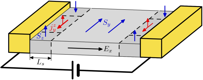
Figure 1: (color online) In a spin-Hall bar setup, the electric current is driven through 2DES contacted by the metallic leads connected to a voltage source. The electric field $E_{x}$ creates an in-plane spin polarization $S_{y}$ in the bulk. Spin currents $j_{y}^{z}$ are running in the vicinity of the contacts while vanishing in the bulk. Out-of-plane polarization $S_{z}$ is accumulated at the sample corners.

However, near the contacts where the spin polarization deviates from its bulk value, the spin current is non-zero. Using the expression (20) in Eq. (23), we find that the spin current near the contacts decays as ($\zeta\ll 1$),

$$j^{z}_{y}(x)=-\frac{eE}{2\pi}~{}\zeta^{2}e^{-{x}/{L_{s}}}\ .$$ (24)

For a sample of finite width, this spin current should lead to a spin accumulation within a distance $L_{s}$ of the corners of the sample, with a component of ${\bf S}$ along $\pm{\bf z}$, as illustrated in Fig. 1.

Note, that for a non-uniform system in thermal equilibrium, where ${\bf E}_{\text{eff}}=0$, the spin density given by Eq. (Spin current and polarization in impure 2D electron systems with spin-orbit coupling) is zero, as well as the spin current. Small equilibrium spin currents R , proportional to $(\alpha/v_{F})^{3}$, are beyond the approximation used when deriving Eq. (23). Our derivation of the diffusion equation (14) and the spin-current (23) relies on the approximation (3) that neglects contributions from diagrams with crossed impurity lines (ladder approximation). This is usually justified provided that $E_{F}\tau\gg 1$. In an infinite system the result (23) is equivalent to a calculation within the Kubo formalism with the first term representing a single-loop contribution and the second term originating from the ladder impurity diagrams.

To reconcile our result for spin current with the predictions of Refs. SCN , it is helpful to consider the ac spin-Hall effect IBM . When the applied electric field is time-dependent, spin polarization is retarded with respect to the field, due to the finite spin relaxation time. As a result, the spin polarization contribution in Eq. (23) does not exactly cancel the electric field contribution, and spin-Hall conductivity becomes non-zero. Solving Eq. (10) for the homogeneous infinite system and generalizing Eq. (22) for a time-dependent state, we find,

$$\sigma_{sH}(\omega)=\frac{e\Delta^{2}}{2\pi}~{}\frac{\omega\tau}{\omega\tau[4\Delta^{2}-(\omega+\frac{i}{\tau})^{2}]+2i\Delta^{2}}\ .$$ (25)

For low frequencies, $\omega\tau_{s}<1$, the spin-Hall conductivity remains small, $\sigma_{sH}\sim-i\omega\tau$. When the frequency exceeds the spin relaxation rate ($\omega\tau_{s}\geq 1$), $\sigma_{sH}$ reaches its maximum value $e\tau/(4\pi\tau_{s})$. For clean samples, this is the universal value $e/8\pi$ predicted in Refs. SCN , while for dirty samples ($\zeta\ll 1$) the maximum value of the spin-Hall conductivity remains strongly suppressed, $\sigma_{sH}\approx e\zeta^{2}/(2\pi)$.

To conclude, we derived quantum kinetic equation for 2D electrons in the presence of spin-orbit coupling and short-range potential scattering. We proved that the dc spin Hall effect disappears in a bulk sample, and we computed the spin accumulation in a finite-size system for a wide range of parameters. This work was supported by NSF grants PHY-01-17795 and DMR02-33773.

References

- (1) S. Murakami, N. Nagaosa, and S.-C. Zhang, Science 301, 1348 (2003); Phys. Rev. B 69, 235206 (2004).
- (2) J. Sinova, D. Culcer, Q. Niu, N.A. Sinitsyn, T. Jungwirth, and A.H. MacDonald, Phys. Rev. Lett. 92, 126603 (2004).
- (3) D. Culcer, J. Sinova, N.A. Sinitsyn, T. Jungwirth, A.H. MacDonald, and Q. Niu, Phys. Rev. Lett. 93, 046602 (2004).
- (4) J. Schliemann and D. Loss, Phys. Rev. B 69, 165315 (2004).
- (5) J. Hu, B.A. Bernevig, and C. Wu, Int. Journ. Mod. Phys. B 17, 5991 (2003).
- (6) S.-Q. Shen, Phys. Rev. B 70, 081311(R) (2004).
- (7) N.A. Sinitsyn, E.M. Hankiewich, W. Teizer, and J. Sinova, cond-mat/0310315.
- (8) E.I. Rashba, Phys. Rev. B 68, 241315(R) (2003); cond-mat/0404723.
- (9) J.I. Inoue, G.E.W. Bauer, and L.W. Molenkamp, Phys. Rev. B, 67, 033104 (2003).
- (10) Ye Xiong and X.C. Xie, cond-mat/0403083.
- (11) A.A. Burkov, A.S. Núñez and A.H. MacDonald, cond-mat/0311328; the spin-density coupling term to be brought in accordance with our Eq. (15) in the published version.
- (12) O.V. Dimitrova, cond-mat/0405339 v.1; results were corrected in v.2 and the vanishing of spin-Hall conductivity was confirmed.
- (13) L.S. Levitov, Yu.V. Nazarov, G.M. Eliashberg, Sov. Phys. JETP 61, 133 (1985).
- (14) V.M. Edelstein, Solid State Commun. 73, 233 (1990).
- (15) F.T. Vas’ko, JETP Lett. 30, 540 (1979); Yu.A. Bychkov and E.I. Rashba, J. Phys. C 17, 6039 (1984).
- (16) J. Rammer and H. Smith, Rev. Mod. Phys. 58, 323 (1986).
- (17) A.A. Abrikosov, L.P. Gorkov, and I.E. Dzyaloshinskii, Methods of Quantum Field Theory in Statistical Physics, (Dover, New York, 1975).
- (18) E.G. Mishchenko and B.I. Halperin, Phys. Rev. B 68, 045317 (2003).
- (19) M.I. Dyakonov and V.I. Perel, Sov. Phys. JETP 33, 467 (1971).