Flip dynamics in three-dimensional random tilings
Abstract
We study single-flip dynamics in sets of three-dimensional rhombus tilings with fixed polyhedral boundaries. This dynamics is likely to be slowed down by so-called “cycles”: such structures arise when tilings are encoded via the “partition-on-tiling” method and are susceptible to break connectivity by flips or at least ergodicity, because they locally suppress a significant amount of flip degrees of freedom. We first address the so-far open question of the connectivity of tiling sets by elementary flips. We prove exactly that sets of tilings of codimension one and two are connected for any dimension and tiling size. For higher-codimension tilings of dimension 3, the answer depends on the precise choice of the edge orientations, which is a non-trivial issue. In most cases, we can prove connectivity despite the existence of cycles. In the few remaining cases, among which the icosahedral symmetry, the question remains open. We also study numerically flip-assisted diffusion to explore the possible effects of the previously mentioned cycles. Cycles do not seem to slow down significantly the dynamics, at least as far as self-diffusion is concerned.
Preprint
Key-words: Random tilings – Quasicrystals – Discrete dynamical systems – Connectivity – Diffusion.
1 Introduction
Rhombus tilings in dimensions 2 and 3 have been an interdisciplinary subject of intensive study in the two last decades, both in theoretical solid state physics because of their strong relation with quasicrystals [1, 2, 3], as well as in theoretical computer science or in more fundamental mathematics [4, 5, 6, 7, 8, 9, 10]. Rhombus tilings are coverings of a portion of Euclidean space, without gaps or overlaps, by rhombi in dimension two and rhombohedra in dimension three. The “cut-and-project” process is a standard method [2, 11] to generate such tilings. It consists in selecting sites and tiles in a -dimensional cubic lattice and in projecting them onto a -dimensional subspace with ; is the dimension of the tilings and the difference is usually called their codimension. The class of symmetry of a tiling is related to and and such tilings will be denoted by tilings. Icosahedral tilings that are widely studied in quasycristal science, are tilings of codimension 3. We consider in this paper three-dimensional tilings of codimensions ranging from 1 to 4. We also make incursions in the general case whenever it is possible.
The “generalized partition” method used in this paper to generate tilings is a variant of the previous one which has proven useful in several circumstances to manipulate and count them [12, 13, 14, 15, 7, 16, 17]. The principles of the method will be recalled below. However, we should already mention that the tilings generated by this technique have specific fixed boundaries. They are polygons in dimension 2 and polyhedra in dimension 3, all of them belonging to the class of zonotopes [18].
As compared to perfect quasiperiodic rhombus tilings, such as the celebrated Penrose tilings [4], the so-called “random tilings” [3] have additional degrees of freedom, the localized phasons or elementary flips, which consist of local rearrangements of tiles (groups of 4 tiles in dimension 3). The activation of these degrees of freedom gives rise to a large amount of accessible configurations which are responsible for a macroscopic configurational entropy, the calculation of which is in itself a difficult topic that the present paper does not address directly.
Among the many problems that remain unsolved in this field, results on flip-dynamics are scarce in three dimensions [19, 20, 21, 22, 23, 10] and are either purely numerical or based upon an approximate Langevin approach. And yet it is a crucial issue in quasicrystal science where elementary flips are believed to play an important role because they are a new source of atomic mobility. They could bring their own contribution to self-diffusion [24] in quasicrystalline alloys and they are involved in some specific mechanical properties, such as plasticity related to dislocation mobility [25] (see subsection 7.1 for a more detailed discussion).
The present paper addresses two issues related to flip dynamics: connectivity of tiling sets via elementary flips and self-diffusion (of vertices) in random tilings when flips are activated.
The question of the connectivity of tiling sets via elementary flips still resists investigation in spite of the apparent simplicity of its formulation: is it possible to reach any tiling from any other one by a sequence of elementary flips? Even if proving that tiling sets are connected via elementary flips is only a first step towards the full characterization of flip dynamics, it is a challenging question that must imperatively be addressed before tackling more complex issues such as ergodicity, self-diffusion, calculation of ergodic times [26, 10] or dislocation mobility. This connectivity issue is also crucial in the context of Monte Carlo simulations on tilings: it is a fundamental ingredient if one hopes to sample correctly their configuration spaces.
So far, connectivity has only been conjectured by Las Vergnas about 25 years ago in the context of “oriented matroid theory” [27]. It remains an open problem in pure mathematics ([28], Question 1.3). In two dimensions, connectivity can be established [5, 6], but the proofs are very specific to dimension 2 and cannot be adapted to dimensions 3 and higher. In reference [16], a new proof of the connectivity in dimension 2 was proposed and the reason why this proof could not be easily extended to higher dimensions was clearly identified: there appear “cycles” (defined below) in the generalized partition method which locally suppress a fraction of flip degrees of freedom. It is this point of view that we shall adopt in the present paper: we shall demonstrate that the obstacles to the generalization of the latter proof can be rigorously bypassed in many cases: in codimensions 1 and 2; in most cases in codimensions 3 and 4. We say “most cases” because a new difficulty arises when one studies three-dimensional rhombic tilings: for a given codimension, all edge orientations are not equivalent. There are 4 non-equivalent edge orientations in codimension 3 and 11 ones in codimension 4. The paper discusses this non-trivial issue in great detail. There is a minority of edge orientations where we are not able to prove connectivity. Note that when all edge orientations are not combinatorially equivalent, the corresponding polyhedral fixed boundaries are not topologically equivalent either. This point will also be discussed in detail in the paper.
Beyond connectivity, the previously mentioned cycles are likely to affect ergodicity. Since they suppress some flip degrees of freedom, they are susceptible to slow down the dynamics and to be responsible for entropic barriers which could for instance prevent a tile from finding its average equilibrium position in the tiling. We have chosen to study self-diffusion of vertices to explore such possible effects because of its physical interest. Self-diffusion has previously been studied in icosahedral tilings [21, 22, 23] but the effect of cycles themselves has never been investigated. We shall see that there are no significant differences in the diffusive behavior between tilings where cycles exist and those where we are able to prove that they cannot exist, nor between tilings where connectivity can be proven and those where it remains open. No sub-diffusive regimes at long time are observed whatever the tilings under consideration. Cycles do not seem to slow down the dynamics, at least as far as self-diffusion is concerned.
The paper is organized as follows: In section 2, we describe the “generalized partition” method used throughout the paper to code the tilings and we explain how “cycles” emerge in this formalism. In the following section 3, we set the basics of flip dynamics, and we discuss the possible influence of cycles on the dynamics by flips. Section 4 discusses the question of non-equivalent edge orientations and related fixed boundaries. In section 5, we give our main theorem that states that cycles cannot exist in favorable conditions, which enables us to prove connectivity by flips in a large variety of cases. When cycles exist, we also study how abundant they are and we derive a simple mean-field argument to account for our observations. In addition, we make a brief incursion into order theory: we prove that the tiling sets have a structure of “graded poset”. In section 6, we discuss how our results on fixed-boundary tilings can be transposed to the more physical free-boundary ones. Finally, section 7 is devoted to a numerical study of the diffusion of vertices. The last section 8 contains conclusive remarks and open questions.
2 Tilings, generalized partitions and cycles
In this section, we present the concept of generalized partition used in the paper to code and manipulate rhombus tilings. This technique was introduced in [12, 13, 14], developed in [15, 16] and mathematically formalized in [7]. The end of the section is devoted to the definition of cycles. We provide a commented example.
2.1 Generalities
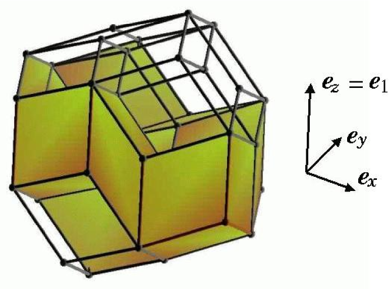
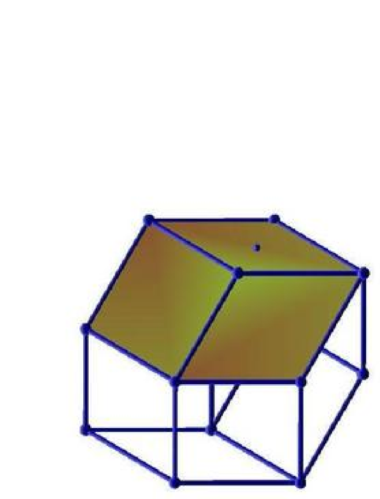
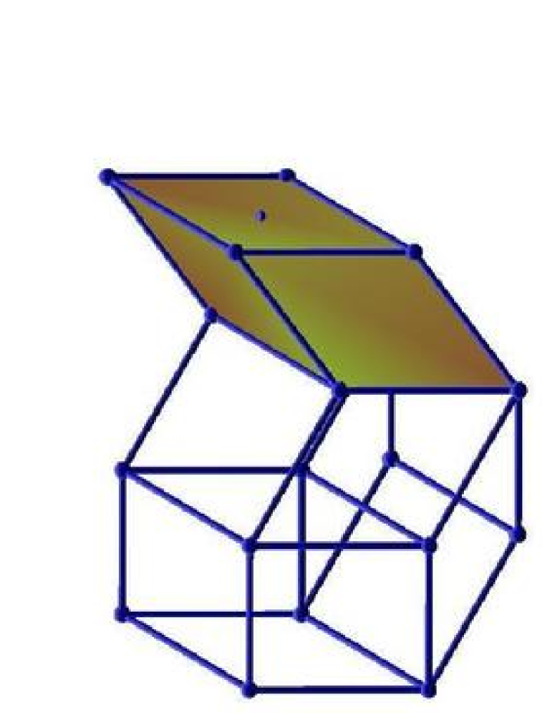
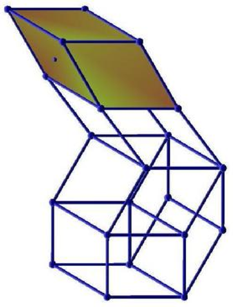
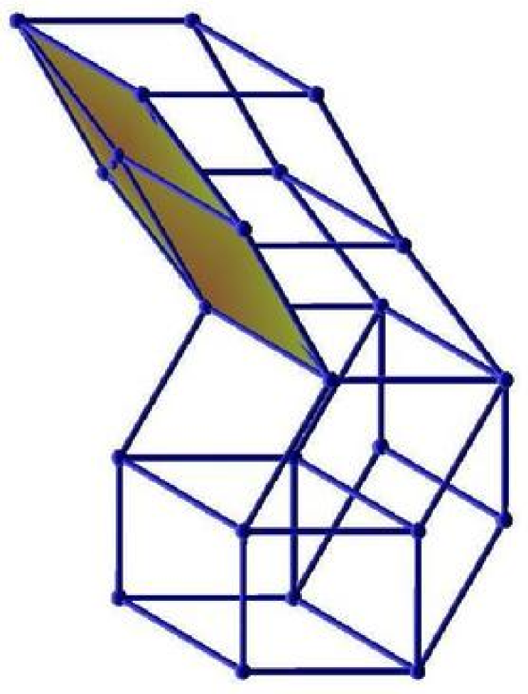
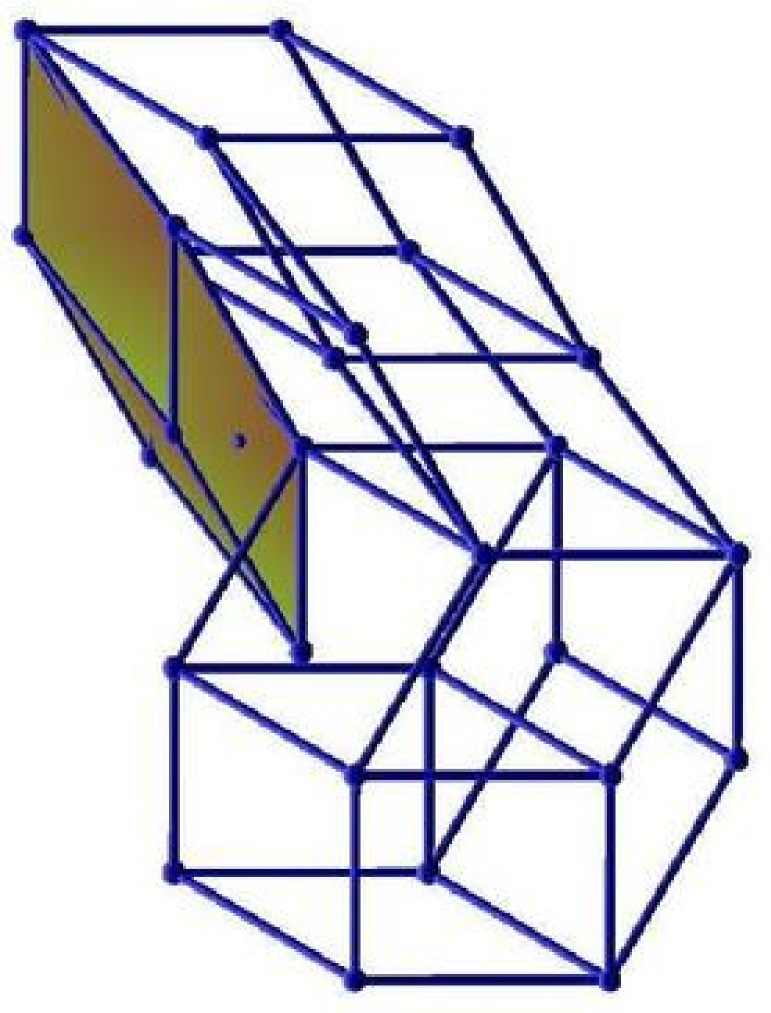
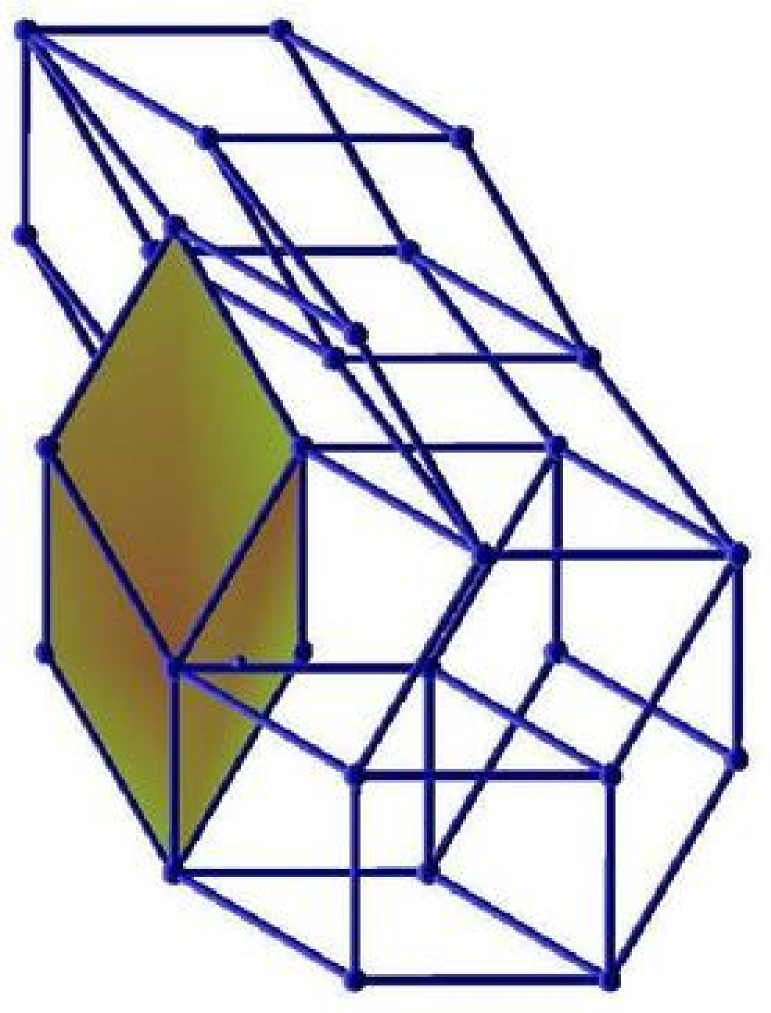
The rhombus tilings considered in this paper (see an example in figure 1), whatever their dimension, have possible edge orientations (belonging to ), denoted by , . They are inherited from the directions of the cubic lattice of during the “cut-and-project” process. Each possible edge has the orientation and norm of one of the vectors . The signs of these vectors are irrelevant and can be arbitrarily chosen. A rhombic tile is defined by of these edge orientations. To avoid flat tiles, the family of orientation vectors is supposed to be non-degenerate: any of them form a basis of .
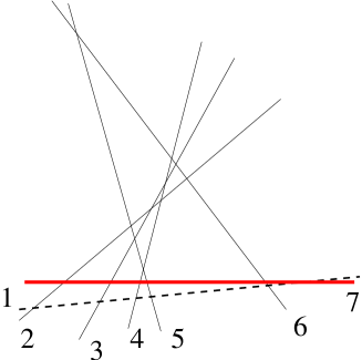
A dual representation of rhombus tilings was introduced by de Bruijn [29, 30]. It consists in seeing the tiling as a grid of lines (see figure 2, right). A line in a tiling is a succession of adjacent tiles sharing an edge (in dimension 2) or a face (in dimension 3) with a given orientation. It is always possible to extend these lines through the whole tiling up to a boundary tile. These lines are called “de Bruijn lines”. In dimension , one can also define de Bruijn surfaces which can be represented by adjacent tiles sharing an edge with a given orientation (see figure 1). They will play an important role below. It exists one family of surfaces, denoted by , for each orientation of edges. There are surfaces in the family . De Bruijn surfaces of the same family do not intersect. A tiling with orientations of edges on a -dimensional space will be called a tiling, and defines its codimension. In dimension , the de Bruijn surfaces are replaced by -dimensional hyper-surfaces.
In this paper, we will mainly be interested in the case , and we shall use -dimensional tiling examples to facilitate the comprehension. In dimension , a rhombic tile is given by the intersection of three surfaces of different families, and so all the different types of tiles are given by all the possible intersections of surfaces of different families; there are different species of tiles. We can prolong any de Bruijn surface of family beyond the tiling boundaries and up to infinity, by a surface perpendicular to the direction far from the tiling. If the tiling corresponds to a complete grid, which means that any three surfaces of different families have a non-empty intersection, it will have fixed boundary conditions. More precisely, this boundary will be a zonotope [18], that is to say the shadow of the hypercube of sides in the -dimensional space onto the -dimensional space, where we recall that the are the numbers of hyper-surfaces in family . We shall describe more precisely this kind of boundaries in section 4 and we shall discuss their relationship with free boundaries in section 6.
Here we make an important remark about de Bruijn surfaces: a -dimensional de Bruijn surface in a tiling is topologically equivalent to a tiling. For example, a de Bruijn surface in a 3-dimensional tiling can also be seen as a 2-dimensional tiling. Indeed, let us consider the trace on of the -dimensional de Bruijn grid dual of : it is a grid made of families of -dimensional surfaces. This grid is complete because the original grid is. It is the dual of a tiling with fixed zonotopal boundaries. In figure 1, a de Bruijn surface is represented. The equivalent 2-dimensional rhombus tiling is obtained by looking at the surface from the direction .
A tiling will be called “unitary” if it contains one de Bruijn surface per family ( for all ). It will be called “diagonal” if it contains the same number of de Bruijn surfaces in each family ( for all ).
2.2 Generalized partitions
Here we introduce the notion of generalized partitions which plays a central role in the paper. We also explain how an edge orientation orients the faces of a tiling. This notion will be fundamental in the proof of connectivity.
The idea of the generalized partitions method is to build iteratively the tiling, by reconstructing the dual grid. In dimension , beginning with a complete grid made by only three families of surfaces, which is unique and represents a periodic tiling made by one type of tiles, we have to describe where to place the de Bruijn surfaces of the fourth family relatively to the existing intersections of surfaces. In terms of tilings, it means that we have to describe where to place the fourth surfaces of tiles on the existing tiling. And iteratively, to build a tiling, we have to describe where to place the family of surfaces on a previously obtained tiling. In order to obtain a tiling by this process, we have to impose some constraints on the way we place the next family of surfaces at each step. The surfaces of one family cannot intersect. No more than surfaces can cross at the same point, otherwise the tile at this point cannot be properly defined. Furthermore, de Bruijn surfaces are directed [15]. Indeed, by construction, they always cross edges with a given orientation, and can be seen as mono-valued functions defined on the hyper-plane perpendicular to their orientation vector (see figure 1).
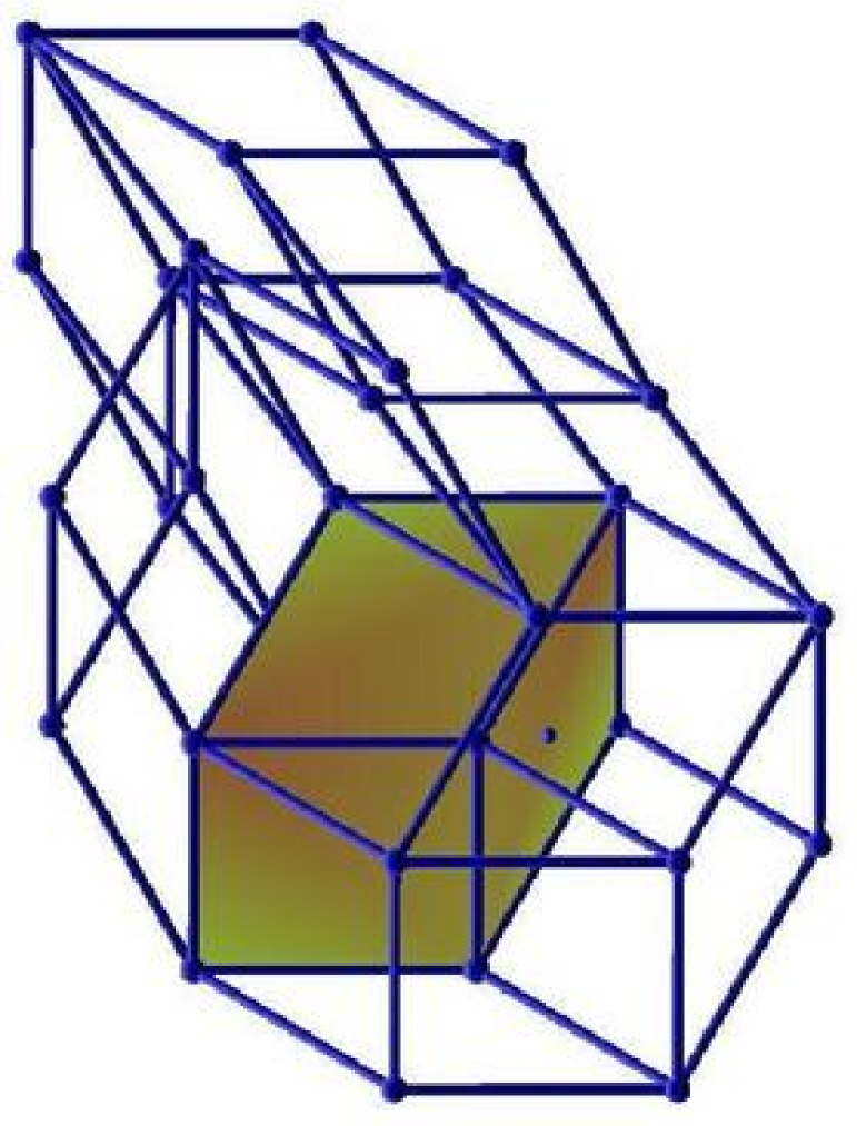
Let us now introduce (see figure 2) how one can define a partial order relation between the tiles of a tiling in order to satisfy these constraints. Since the de Bruijn surfaces of a family do not intersect, they divide the space in disjoint domains. Furthermore, since de Bruijn surfaces are globally oriented, we can index these domains from 0 to such that, following the direction given by we go through all these domains in an increasing order. We denote these domains by and the surfaces of by . The de Bruijn surface lies between the domains and . In other words, if we consider a tiling , and if we particularize the de Bruijn surfaces of the family (see figures 1 and 2), tiles not belonging to the surfaces of are distributed between the different domains.
Now we contract (or delete) the tiles of from the tiling by setting the length of to 0, thus obtaining a tiling . Two adjacent tiles of , with one above the other along the direction , are either on the same domain or separated by one (or several) de Bruijn surface of , the tile atop being in the higher domain. This allows to define an order relation, , relatively to , between any two adjacent tiles and in : means that is below along and so that is either in the same domain as or in a lower domain.
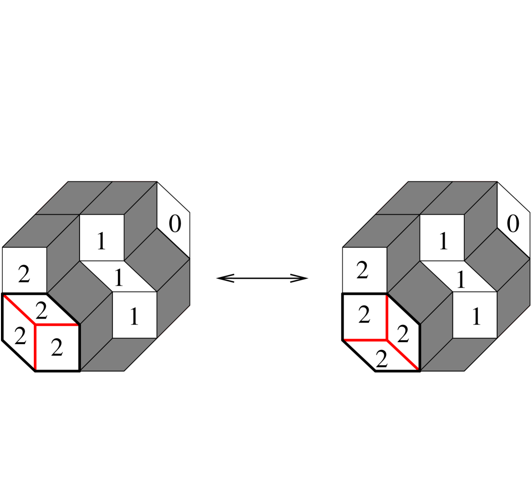
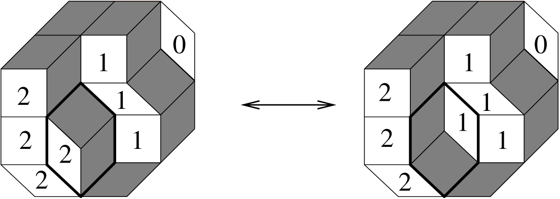
We can recover this order relation between any adjacent tiles by orienting all the faces111In this paper we call face of a tile a -dimensional polyhedron generated by orientation vectors. of a tiling by : given two adjacent tiles and of , if when one goes from to , the face between and is crossed in the positive direction (see figure 3). We say that the vector orients the faces of .
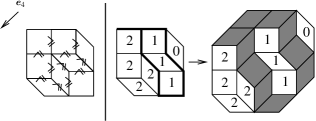
Now remind that our aim is to code the position of the de Bruijn surfaces of on a tiling . One way to do that, is to associate an integer , , called a part, to each tile of the tiling : is equal to the index of the domain the tile belongs to. For example, one tile with a part equal to is on the third domain, so between the second and the third de Bruijn surface of the family ; A tile with a part equal to zero is below the first surface. These parts have to respect the partial relation order , which for convenience we will simply denote by in the following of this paper. To generate all the possible tilings from a one, we have to find all the possibilities of filling the tiles of the latter tiling by parts from to respecting the partial order between the tiles. This type of problem is called a generalized partition problem of height on the tiling. A solution of this problem is called a (generalized) partition. In the figure 2, one can see an example of a tiling coded by a generalized partition on a tiling. The underlying tiling is called the base tiling of the generalized partition problem.
To sum up, there is a one-to-one correspondence between tilings and pairs composed of a base tiling together with a generalized partition on this base tiling. This one-to-one coding of zonotopal tilings is described in a more formal way in references [7, 16]. It can be iterated by induction on to code tilings, starting from the simplest case of partitions on tilings. The latter can be seen as 3-dimensional rectangular arrays and the corresponding partition problems are usually called solid partition problems [15].
To close this section, let us remark that when one codes tilings by the generalized partition technique, the order in which the de Bruijn families of surfaces are successively added to the tilings is arbitrary. For sake of convenience, one is for example free to choose the first edge orientations defining the base tilings among the possible ones. Of course, the set of base tilings depends on this choice.
2.3 Definition and examples of cycles
We can now define what we call a cycle on a base tiling [16]. A cycle is a succession of pairwise adjacent tiles, , such that: with respect to the previous order relation on tiles, as it is illustrated in figure 3. That means that the parts of the tiles inside the cycle have to be equal to a unique part and have a collective behavior. In particular, their values cannot but change simultaneously. Such cycles are known to exist on specific ad hoc examples. The first one can be found in reference [31] (example 10.4.1) and the second one in [32] (example 3.5), in the context of “oriented matroid theory”. Figure 3 provides another example. Our analysis below shows that cycles already exist in tilings, but not in unitary ones. A base tiling with cycles is said to be cyclic, and conversely a tiling without cycles is acyclic.
Geometrically speaking, a cycle is a sequence of tiles making a loop such that each tile is placed above the preceding one relatively to the orientation prescribed by . In the example of figure 3 this vector is placed perpendicularly to the picture plane. This cycle can be seen analogously to a loop of coins, each one placed above the preceding one. A visible consequence is that we cannot place a de Bruijn surface of between the tiles of the cycle, as well as we cannot place a horizontal sheet of paper between the coins, splitting the loop between coins above the sheet and below the sheet. A de Bruijn surface of is either completely above or completely below a cycle. Which is equivalent to say that the tiles must bear equal parts.
|
|
|
|---|---|---|
|
|
|
|
|
|
One of our purposes below is to analyze the occurrence of cycles in a more systematic way. In addition, in the following of this article, we will discuss the possible influence of these cycles on the configuration spaces of tilings and on flip dynamics. Let us emphasize that this problem is specific to dimensions and above, since there cannot exist cycles in dimension [31, 32].
3 Basics of flip dynamics
Before discussing in further details the consequences of these cycles, we now describe flips in rhombus tilings, and what they become in the generalized partition viewpoint.
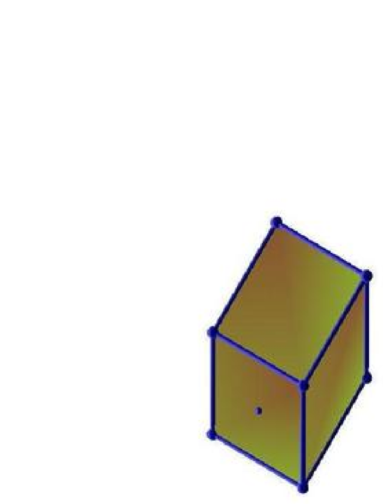
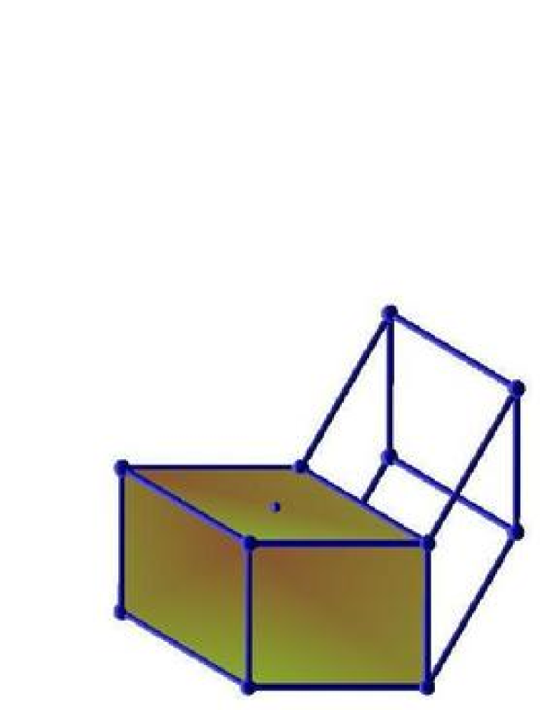
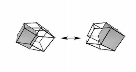
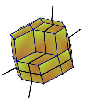
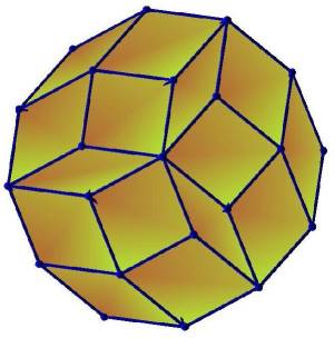
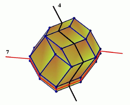
One can define in rhombus tilings local degrees of freedom which are called elementary flips or localized phasons. In dimension , a flip consists of a local rearrangement of tiles in a small zonotope inside the tiling. In dimension it is a rearrangement of tiles inside a hexagon, and in dimension , of tiles inside a rhombic dodecahedron, see figures 4 and 5. In dimension the configuration space of tilings is proven to be connected via these elementary flips [5, 6, 16]. Which means that we can go from any tiling to any other one by a finite sequence of flips. In dimension , it is an open question that we shall address in this paper.

Flips allow to define a Monte Carlo Markovian dynamics on tiling sets as follows [19, 33]: pick up a tiling vertex at random with uniform probability. If this vertex is flippable (it is surrounded by tiles in dimension ), then flip it. This Markovian process converges towards the uniform distribution on the set of tilings provided the configuration space is connected by flips. Note that temperature can be introduced in this point of view to take into account possible interactions between tiles; the transition rates must be adapted consequently. In this paper, we focus on the infinite temperature limit, where all the configurations have equal equilibrium probability and where all rates of allowed transitions are equal.
This Markovian dynamics has been mainly studied in dimension 2. It has been demonstrated that it is rapid in codimensions 1 [34] and 2 [26]. This means that the typical times to reach equilibrium are polynomial in the system size. The same kind of result has also been established numerically in the case [10]. In addition, there exist studies concerning diffusion in random tilings evolving via this Markovian dynamics. This last point will be discussed in great detail in section 7.
Now, let us see how these flips are seen in the generalized partition point of view. On a generalized partition problem on a tiling, which codes a tiling, flips can be classified into two types (see figure 5), following reference [16].
Type-I flips involve only tiles of the base tiling and no tile of the de Bruijn family . As a consequence, the tiles bear equal parts, and these flips only change the base tiling without modifying the parts of the tiles. Type-II flips involve tiles belonging to the de Bruijn family . More precisely, they involve tiles having an edge oriented by , locally representing a surface of the family , and one tile of the base tiling. Such a flip consists in modifying the position of the latter surface with respect to the tile . So it changes the part borne by the tile by .
One can now build a schematic picture of the configuration space of tilings [16] (see figure 6). Considering tilings, one can split up the configuration space into disjoint fibers. A fiber contains all the tilings generated by the same generalized partition problem, that is to say which have the same base tiling. Type-II flips keep the base tiling, and therefore the fiber, unchanged, whereas type-I flips change the base tiling and therefore the fiber. The set of all fibers is called a fibration. For a given configuration space, there are different fibrations corresponding to the choice of among the edge orientations.
Using this picture, one immediately gets the following result: if fibers are all connected and if the base is connected itself, then the configuration space is connected in its turn. Indeed, the connectivity of fibers allows one to put all the tiles of the tiling to the same part value (for example 0), thus releasing all type-I flips on the base tiling and allowing to go to any fiber.

Now it is established in B that a fiber corresponding to an acyclic base tiling is connected, because it is possible to change the parts on tiles one by one. Therefore if all base tilings are acyclic and if the base is connected, then the configuration space is connected in its turn. Since there cannot exist cycles in dimension 2, sets of tilings are always connected [16]. We shall follow this route in the following to prove connectivity in a wide variety of cases.
What happens when there are cycles? A cycle in a tiling is a sequence of pairwise adjacent tiles that are geometrically constrained to bear the same part in the generalized partition problem. In term of flips, since all parts of the cycle are forced to be equal, the tiles of a cycle cannot participate to a type-II flip which would change the part of a single tile to a value different from that of the whole cycle.
In other words, a de Bruijn surface of cannot pass through a cycle, because it is constrained to be completely above or completely below the cycle. In order to allow the surface to pass the cycle, one must break beforehand the cycle by type-I flips, if it is possible. The tiling is locally jammed.
A direct consequence is that a fiber based on a tiling with cycles cannot be connected anymore by single flips. We must modify our schematic picture of the configuration space: there are connected fibers based on tilings without cycle, as well as disconnected ones based on tilings with cycles. The connectivity is not obvious anymore (see figure 7).

Let us anticipate on the following to emphasize that these cycles should have an influence not only on the connectivity but also on the Markovian flip dynamics. Indeed they forbid some type-II flips, they reduce locally the degrees of freedom related to those flips because of jammed clusters of tiles. They are susceptible to slow down the dynamics, in the sense of an increase of ergodic times. In the schematic picture of figure 7, one can see that the cycles make the configuration space more intricate. One can imagine that they could create inhomogeneities in the distribution of flip paths through the phase space resulting in entropic barriers. More precisely, in [26], the demonstration of short ergodic times in dimension was based on short ergodic times inside the fibers, which is not possible anymore in presence of cycles. Therefore, one can wonder whether the features of the dynamics are modified by those cycles. It will be the purpose of section 7.
4 Edge orientations, line arrangements and boundaries
Before tackling the questions of connectivity and vertex diffusion, this section clarifies the question of non-equivalent edge orientations in 3-dimensional tiling problems and their relation with zonotopal boundaries. Indeed, it will appear in the following that the existence (or not) of cycles in base tilings is closely related to the choice of edge orientations. In particular, we shall be able to prove connectivity by flips for a large majority of edge orientations, but the proof will fail in some minority cases. The classification of edge orientations will be related to a classification of line arrangements in the projective plane .
4.1 Edge orientations and equivalence relation
Random tiling model studies concern the way of arranging simple geometrical structures (the tiles) in the space or in the plane. One possible interest is the contribution to the entropy of such possible configurations. Here we are interested in the way the system can go from one of those configurations to another. The geometry of the tiles does not concern directly those features but rather the symmetries. Indeed, one can imagine to start with a tiling and begin to vary slightly one vector . It will deform globally the tiling, but not its topological structure in terms of relative positions of the tiles. More precisely, vectors can be rotated or elongated provided a modified vector does not cross a plane made to by two other ones, which means there exist no flat tiles and no tiles are overlapping.
Given two families of edges, denoted by and , we define them as equivalent [35] if one can transform into by the composition of the three following transformations: (i) permutation of the indices; (ii) sign reversals; (iii) continuous deformation of the vectors without creating degenerate configurations of three vectors: for all . In dimension 2, all families of edges are equivalent. When the families and are equivalent, we say that they define equivalent sets of rhombic tiles.
4.2 Line arrangements
To distinguish and enumerate the non-equivalent families of edge orientations, we map families of edges on line arrangements in the projective plane (see [35] for more details). We proceed as follows. The set of edges are represented by a family of vectors . Recall that the signs of those vectors are irrelevant. Those families of vector arrangements are in bijection with arrangements of planes , such that for all , is orthogonal to and each contains the origin. For one given arrangement, since all the planes pass through a common point (i.e. the origin), one can get all the information on it by its trace on the projective plane (which is conveniently represented by an affine plane that does not contain the origin. Then this trace is made of lines defined as the intersections of the projective plane and the ). So, one can differentiate vector arrangements by differentiating the line arrangements in the projective plane.
We precise now in the line arrangement point of view what equivalent families of edge orientations become. Two line arrangements with indexed lines will be equivalent if they only differ by a re-indexation of the lines and continuous geometric transformations on the lines which do not create triple points, because a triple point corresponds to three coplanar vectors , , . The equivalence classes of line arrangements in the projective plane, from to lines, are given by Grünbaum [36] and are displayed in figure 8. We use in the following the indexation of line arrangements of this figure 8. There exists only one arrangement of four and five lines, whereas there exist four arrangements of six lines and eleven arrangements of seven lines, which correspond to as many different , , , and random tiling problems. The icosahedral symmetry belongs to the equivalence class of the first arrangement of six lines.

4.3 Polyhedral boundaries
In the following, we study the presence of cycles in tilings associated with all those line arrangements. But let us first discuss how those line arrangements are related to the boundary of the tilings we are considering.
The boundary of the tiling generated by the partition-on-tiling method is the boundary of the Minkowski sum of the vectors :
| (1) |
which is also called the zonotope generated by the vectors [18, 15] (in dimension 2, this zonotope is always a -gon of sides , which is reminiscent of the uniqueness of edge orientations). Zonotopes are convex and centro-symmetric. This boundary is uniquely determined by the choice of the edge configurations, and thus by the choice of the line arrangement in dimension 3. One can directly see this line arrangement by seeing one hemisphere of the boundary of a unitary tiling projected on a plane (see figure 9). The corresponding line arrangement is made by the line crossing each family of edges. The projection of the boundary hemisphere can be seen as a tiling and the previous line arrangement can be seen as its de Bruijn grid. These lines are not straight but they can be stretched without changing the crossing topology. Indeed this line arrangement can also be seen as the trace on the projective plane of de Bruijn grid dual of a tiling filling the zonotope. By definition, the boundary does not depend on the tiling inside this boundary. The line arrangement corresponding to the boundary can always be seen as the trace of the dual de Bruijn grid made by flat de Bruijn surfaces, which always represents a possible tiling. In the figure 9, one can see two tiling boundaries corresponding to the icosahedral tiling and to the fourth line arrangement with six lines. In particular these two boundaries differ by the existence of a vertex of connectivity six in the right-hand-side one. This is seen in the dual fourth line arrangement by the presence of one hexagon. By contrast, the total number of tiles does not depend on the choice of the boundary because the de Bruijn grid is complete:
| (2) |
To characterize the differences between random tilings with non-equivalent edge orientations, we have enumerated tilings with unitary boundaries (i.e. with one de Bruijn surface per family), see tables 1 and 2 . For unitary tilings it is possible to span all the configuration space for each boundary condition. Indeed, we demonstrate in the following that the configuration space of all the random tilings with unitary boundaries are connected for codimensions up to which are under interest in the present paper. These results, which are exact, show definitively that tiling problems with non-equivalent families of edge orientations cannot be put in one-to-one correspondence since they do not have the same number of configurations. There are 160 unitary tilings built on the first 6-line arrangement, that is to say with icosahedral symmetry.
| Unitary tiling space | ||||
|---|---|---|---|---|
| Line arrangement | 1 | 2 | 3 | 4 |
| Tilings | 160 | 148 | 144 | 148 |
| Unitary tiling space | |||||||||||
|---|---|---|---|---|---|---|---|---|---|---|---|
| Line arrangement | 1 | 2 | 3 | 4 | 5 | 6 | 7 | 8 | 9 | 10 | 11 |
| Tilings | 7686 | 8260 | 7624 | 7468 | 7220 | 7690 | 7518 | 7242 | 7106 | 6932 | 6902 |
5 Connectivity and structure of the configuration space
This section contains results concerning the configuration space of 3-dimensional tilings. First we formulate our main theorem in 5.1. It gives a general sufficient condition to prove that base tilings are acyclic. We apply this result to dimension 3 in 5.2 to prove that most line arrangements in codimension up to 4 generate connected tiling sets. Then we considerer in 5.3 the opposite situation where cycles exist and we study how abundant they are. A mean-field argument supported by numerical simulations shows that, in this case, cyclic tilings are generic and acyclic ones are exceptional at the large size limit. Then in 5.4 we characterize the structure of the configuration space in the frame of order theory.
5.1 Connectivity: Main theorem
The results of this subsection are not specific to dimension 3 and can easily be adapted to any tiling problem. However, for sake of simplicity, we shall write our theorem and its proof in dimension 3. Our goal is to give a sufficient condition to prove that base tilings are acyclic.
We consider a tiling problem defined by a family of edge orientations. The set of all the possible tilings of this tiling problem is denoted by . Tilings of are coded by generalized partitions on base tilings defined by the first edge orientations and the faces of which are oriented by . The set of base tilings is denoted by . To formulate our main theorem, we first need introducing some new notions.
First of all, we say that the family is acyclic if any base tiling (of any size) of edges , the faces of which are oriented by , is acyclic.
A family of indices , , is attached to each tile of a base tiling as follows. For each family of de Bruijn surfaces , if belongs to a surface of , then the index is equal to . If lies between the surfaces and , in the domain , then is half-integer and is equal to . Let us remark, that when we code a tiling, , by a generalized partition on , the parts on each tile of correspond to the domain, defined by the family , they belong to: For the tiles of in , we have .
For each , defines a function on the partially ordered set of the tiles. We say that is monotonous increasing if given any two tiles and , if then . Note that we can in a similar way define the notion of monotonous decreasing , which is equivalent to the previous one up to a sign reversal of .
We also define companion vectors in the family : any two vectors and in are said to be companion if either and orient equivalently all the faces made by the remaining vectors of , or and do.
We shall prove below the following lemma:
Lemma: if and are companion vectors in the family of edge orientations , then the function is monotonous (increasing or decreasing).
As a consequence, in this case, cannot but be constant along a cycle. Therefore a cycle either lies entirely in a single de Bruijn surface of (if is an integer) or strictly lies between two of them (if is half-integer). In the first case, the cycle lives in the equivalent of a tiling (see section 2.1), and in the second case in a tiling of edge orientations . We already know that cycles do not exist in any tiling. Therefore if we can prove inductively that cycles cannot exist in the tilings (in other words that is acyclic), we get that they cannot exist in base tilings under interest. We are led to our main theorem:
Main theorem: Given a family of 3-dimensional edge orientations , if there exists a vector in companion of , and if the family is acyclic, then is acyclic in its turn.
This theorem will be used in the following subsection as follows: we shall prove that some families of edges are acyclic, proceeding by induction on their numbers of vectors. Connectivity of all fibers in the fibration corresponding to will follow. If in addition we know that the set of base tilings is connected, we shall get the connectivity of the whole set of tilings .
To finish with, we prove our first lemma. We prove that if and orient equivalently all the faces made by the remaining vectors, then is monotonous increasing. We could prove in a similar way that if and orient equivalently all the faces made by the remaining vectors, then is monotonous decreasing.
To establish the monotony of , on all the tilings based on the family , we consider two adjacent tiles and such that (i.e. ). Three cases may occur: (i) and belong to two different de Bruijn surfaces of family . Since , and companion of , is above along the direction , then ; (ii) belongs to a de Bruijn surface of and belongs to a domain between two such surfaces; or belongs to such a domain and belongs to a de Bruijn surface. In both cases, for the same reasons as in (i), ; (iii) and belong to the same domain or to the same de Bruijn surface : . Therefore, in all cases, , which proves monotony.
5.2 Connectivity in dimension 3
We now exhibit a criterion to identify companion vectors in the line arrangements in the projective plane corresponding to families of 3-dimensional edge orientations. Since any vector in can a priori play the role of , we seek any two companion vectors in .
In order to find companion vectors, we represent the projective plane by the unit 2-sphere on which antipodal points are identified. The lines on are now represented by great circles on , such that lies in a plane perpendicular to . This circle separates into two hemispheres. We define a positive hemisphere and a negative one such that points from to .
Here we denote by the face species that is defined by the vectors and . It is represented in by the two intersections of the circles and , denoted by and . These points are identified in .
Now we prove that a face , where and are different from and , is oriented equivalently by and if and only if belongs to or to .
We assign the orientation of by , by a unitary vector , normal to , and crossing in the same direction as , that is to say . In other words, . We obtain in the same way that , since and orient equivalently . Now, by definition, is unitary and is perpendicular both to and . Thus it coincides with or . Hence belongs to or to .
Therefore two vectors and are companion if and only if all the points with and different from and belongs to , or all of them belong to (in the case where it is and which orient equivalently all the faces).
In practice to find companion vectors one can use any hemisphere of represented by an affine plane to which we add the line at infinity. If this plane can be chosen so that all the points made by the intersection of two lines different from and are on the same sides of and , then and are companion vectors. An example is displayed in figure 10 (left).
The previous analysis can also be understood geometrically by considering one arbitrary hemisphere of the boundary of a unitary tiling corresponding to a given arrangement, as displayed in figure 10 (right). In this figure, the vector is perpendicular to the figure plane. It orients all the faces from bottom to top. Since the zonotope is convex, one can easily check that in this representation, a companion of this vector is such that the arrangement is completely situated on one side of the line . Whereas a vector such that the line divides the arrangement into two non-empty parts cannot be a companion of . Indeed, if orients the faces on the right of from bottom to top, one can see that it orients the faces on the left of from top to bottom.
We have systematically applied this criterion on the line arrangements of figure 8 to identify companion vectors, in order to apply inductively our main theorem. Tables 3 and 4 provide a summary of our investigations. For each line arrangement, in which the particularized line corresponds to the vector orienting base tilings, a 0 indicates that the corresponding family of edge orientations is acyclic. If for a given arrangement, there exists a for which it is the case, we can conclude that the configuration space is connected after checking that the base is itself connected.
Conversely, there are arrangements for which we cannot find any pair of companion lines. The first arrangement of six lines is an example. It means that we cannot state on the absence of cycles in any generalized partition based on this arrangement. Actually, we will see in the following that we do find cycles on these generalized partitions. In fact, for each arrangements for which we cannot prove the absence of cycles we find them by numerical exploration, see tables 3 and 4, and section 5.3. There exist only three arrangements (among 17) of at most seven lines for which there is no fibration without cycles and the connectivity of which remains open, as it is displayed in the tables. So for all the remaining 14 arrangements, we prove the connectivity of the corresponding tiling sets for any tiling size.
By contrast, sets of unitary tilings are connected for any codimension lesser than 4. Indeed, we proved by systematic numerical exploration of sets of unitary tilings of codimension lesser than 3 that there always exists an acyclic fibration in this case.
In order to prove the connectivity for the tiling problems for which all fibrations exhibit cycles, we would have to prove that one can always break the cycles by type-I flips (see figure 3). Which means that there exists a sequence of flips which brings the tiling from any disconnected fibers to a connected one. Then one can change the parts of the tiles of previous cycles by type II-flips, and bring back the tiling to another component of the initial disconnected fiber. We have not established a possibility to break those cycles in all cases, and therefore the connectivity problem remains open.
In principle, the arguments developed in this section can be extended to any tiling problem using arrangements of hyper-planes in the projective space provided one knows their classification for fixed and . In A, we prove connectivity for codimension 2 tilings of any dimension. Note that independently of this work, and after introducing a new and different formalism, Frédéric Chavanon and Éric Rémila quite recently also established connectivity in codimension 2 [37].
5.3 Abundance of cyclic base tilings ; mean-field argument and numerical studies
We now present numerical results on the abundance of cyclic base tilings of dimension 3 as a function of their boundary size, as well as a mean-field argument to account for these results. In this section, we focus on diagonal tilings: for any . For unitary tilings, we completely cover the configuration space (by use of a deep search algorithm), therefore the results are exact. For larger tilings, we numerically sample the tiling configuration space by use of the Monte Carlo Markovian dynamics described in section 3.
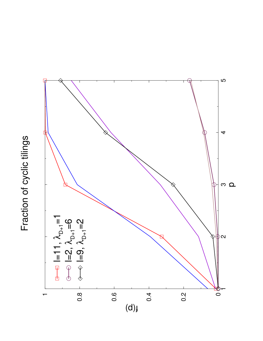
We have made this numerical investigation for all the tiling problems corresponding to 6 and 7-line arrangements, with one particularized line of index corresponding to to orient the base tilings. Typical cycle abundance we found are displayed in figure 11. For all the tiling problems for which we prove that cycles cannot exist we effectively never find them. For the other ones, we find cycles and their occurrence increases rapidly with the tiling size for all cases with a similar law. The differences come from that cycle existence does not arise at the same size for all those tiling problems. In particular, cycles do not exist in unitary tilings (exact result) and they appear starting from . For tilings for which there exist cycles in the unitary case, the cycle fraction is already close to for . These results show that when cycles can exist in a tiling problem, they are certainly very frequent for tilings at large size . Indeed, if a small cycle appears in a small tiling, it will be likely to appear locally in a large one which can be seen in a first approximation as a juxtaposition of nearly independent smaller tilings.
Following this idea, we now propose a mean-field argument to account for these results. For a tiling problem in which cycles are possible, we suppose that there is a non-zero probability that a tile belongs to a cycle. If all the tiles are considered as independent, the probability that no tile belongs to a cycle in the whole tiling is then and the fraction of cyclic tilings reads:
| (3) |
This supposes that is independent of the tiling size. It is necessarily false since we have seen that in some cases cycles appear only starting from a given size. But one can think that it is a good approximation for large sizes. The fits of the measured fraction of cyclic tilings by this simple law reproduce correctly the results in all the cases, see figure 11. A summary of these fits is given in tables 3 and 4. We mention that tiling problems based on the same line arrangement but with a different particularized line are not necessarily different. In particular, the 6 fibrations of the tiling problem corresponding to the first 6-line arrangement are all equivalent because all 6 lines play the same role with respect to the 5 remaining ones. They are represented by the same in table 3.
Concerning the connectivity problem one can see that it remains only three open cases. One of them corresponds to the first arrangement of 6 lines and so to the icosahedral symmetry. Note that it can bias the issue of few results on the fractions of cyclic base tilings in table 4. Indeed, the corresponding base tiling sets might be disconnected and our Monte Carlo sampling might be incorrect. These 3 concerned cases are indicated in bold faces in the table.
| Cycle abundance in base tilings fitted by | ||||||||
| 6-line arrangement number | Particularized line | Connectivity problem | ||||||
| \bigstrut[b] | 1 | 2 | 3 | 4 | 5 | 6 | ||
| 1 | 1.32e-06 | 1.32e-06 | 1.32e-06 | 1.32e-06 | 1.32e-06 | 1.32e-06 | open | |
| 2 | 0 | 0 | 0 | 0 | 0 | 0 | connected | |
| 3 | 0 | 0 | 0 | 0 | 0 | 0 | connected | |
| 4 | 0 | 0 | 0 | 0 | 0 | 0 | connected | |
| Cycle abundance in base tilings fitted by | |||||||||
| 7-line arrangement number | Particularized line | Connectivity problem | |||||||
| \bigstrut[b] | 1 | 2 | 3 | 4 | 5 | 6 | 7 | ||
| 1 | 0 | 0 | 0 | 0 | 0 | 0 | 0 | connected | |
| 2 | N.A | 2.98e-5 | 3.57e-5 | 2.15e-5 | N.A | 1.38e-4 | 1.13e-4 | open | |
| 3 | 0 | 0 | 0 | 7.58e-3 | 0 | 0 | 0 | connected | |
| 4 | 0 | 0 | 0 | 0 | 0 | 0 | 0 | connected | |
| 5 | 0 | 0 | 0 | 0 | 0 | 0 | 0 | connected | |
| 6 | 5.93e-3 | 1.39e-4 | 3.32e-4 | 2.81e-4 | 1.65e-4 | 1.93e-4 | 3.18e-4 | open | |
| 7 | 0 | 0 | 0 | 2.13e-4 | 4.05e-4 | 2.14e-4 | 0 | connected | |
| 8 | 5.01e-4 | 0 | 0 | 0 | 0 | 0 | 0 | connected | |
| 9 | 0 | 1.51e-3 | 0 | 0 | 6.86e-3 | 6.14e-3 | 0 | connected | |
| 10 | 0 | 0 | 0 | 0 | 6.07e-3 | 0 | 0 | connected | |
| 11 | 6.20e-3 | 0 | 0 | 0 | 0 | 0 | 0 | connected | |
5.4 Structure of the configuration space
We now make a brief incursion into graph theory and order theory. The configuration space can be seen as a graph , the vertices of which represent tilings, and the edges of which represent single flips: given two tilings and , is an edge of if and differ by (only) one single flip (see figure 6). We prove that this graph can be embedded in a high-dimensional hyper-cubic lattice , thus generalizing results previously specialized to plane octagonal tilings [16], even in the possible case where is not connected.
As an immediate corollary, we demonstrate that this graph can be given a structure of graded partially ordered set (graded “poset”) [38]. Indeed a partial order relation is associated below to the iterated partition-on-tiling process. Saying that this poset is graded means that there exists a rank function on configurations such that if covers (i.e. is just above) then . This rank function is simply the sum of the (integral) coordinates of a tiling in the lattice . This order has unique minimal and maximal elements.
The present point of view is applicable to tiling sets of any dimension and codimension .
5.4.1 Structure of the graph
We first prove that the configuration space can be seen as a graph embedded in a high-dimensional hyper-cubic lattice . We proceed by induction on the codimension , for any fixed dimension .
In codimension 1, the tilings are encoded by hyper-cubic partitions. The coordinates of a tiling are simply the parts , , of its associated partition and a tiling is therefore naturally represented by a point of integral coordinates in a hyper-cubic lattice of dimension . A flip is encoded by an increase or decrease of the corresponding part by one unit and thus it corresponds to an edge of the hypercubic lattice.
Suppose now that the above property holds for the graph . A tiling is encoded by both a base tiling and a generalized partition on this base tiling. By hypothesis, the base tiling is encoded by integral coordinates , . We denote by , the parts of the partition. We now demonstrate that if is encoded by the coordinates , then is embedded in a lattice of dimension .
The only subtlety comes from the fact that the indices must be correctly chosen with respect to the base tiling , so that is globally embedded in a hyper-cubic lattice (and not only locally), as it is already discussed in reference [16] in the special case of octagonal tilings. We do not reproduce the ideas of this reference which cannot be easily generalized.
A tile of any base tiling is defined as the intersection of de Bruijn surfaces. The de Bruijn families are indexed by and in each family , the surface is indexed by . A tile is now indexed by the indices independently of . We simply fix an arbitrary one-to-one correspondence between these indices and the indices , independent of the tiling .
Now that we have defined the integral coordinates of a tiling, we only need to check that both type-I and type-II flips respect the lattice structure, that is to say that they correspond to an increase or a decrease of (only) one coordinate by one unit.
Type-II flips do not affect the base tiling (the are unchanged) whereas they change exactly one by ; Type-I flips concern the base tiling only: they change one by and tiles of the base tiling move. Since the flip is possible, they all bear the same part value before the flip. After the flip, these part values remain unchanged. Since the tiles involved in the flip bear the same indices before and after the flip, the coordinates remain unchanged. To sum up, either one or one (and only one) is increased or decreased by one unit when a flip is achieved.
5.4.2 Structure of graded poset
When is connected by flips, as far as the order structure is concerned, the previous results ensure that has a structure of graded poset inherited from the order structure of : a tiling is greater than a tiling if all the coordinates of are greater than the corresponding coordinates of in . The rank function is simply the sum of the coordinates of in the lattice . The minimum tiling is obtained when all the parts are set to 0. The maximum tiling is obtained when all the parts are set to their maximum possible value. The same kind of result is also established in [37] in codimension 2.
To close this section, note that the existence of the rank function make in principle possible the application of the technique developed in reference [17] to calculate numerically the entropy of tilings with a given edge orientation, as soon as the configuration space is connected by flips.
6 What about more physical free-boundary tilings?
In reference [17], it is discussed that the fixed boundaries we consider in the present paper are not physical. The aim of the present section is to clarify how our results can be transposed to free- (or periodic-) boundary tilings which are more realistic models of quasicrystals. We argue that flip dynamics in fixed-boundary tilings is relevant to flip dynamics in free-boundary ones provided one focuses on their central regions, where they forget the influence of their polyhedral boundary.
Since [12], it is known that fixed zonotopal boundaries have a strong influence on rhombus tilings. This boundary sensitivity has been widely studied in two dimensions (see references in [17]) and recently numerically explored in tilings [10, 17]. This spectacular effect is generically known as the “arctic phenomenon”, which means that at the large size limit, constraints imposed by the boundary “freeze” macroscopic regions near the boundary. In these frozen regions, the tiling is periodic, contains only one tile species, and has a vanishing entropy. By contrast, the remaining “unfrozen” regions contain random tilings with several tile species and have a finite entropy per tile. In the two-dimensional hexagonal case, the unfrozen region is inscribed in an “arctic circle”. The tiling is not homogeneous inside this circle and presents an entropy gradient.
By contrast, in tilings filling a rhombic dodecahedron, its has been numerically established that the unfrozen region is an octahedron [10, 17], inside which the tiling is homogeneous and the entropy per tile is constant. In other words, inside the octahedron, the tiling is a free-boundary one. This octahedron contains 2/3 of the tiles.
In [17], it is argued that this qualitative difference between two- and three-dimensional tilings is related to the entropic repulsion between de Bruijn lines and surfaces. In dimension 2, it is favorable to bend de Bruijn lines because the bending cost is smaller than the entropy gained by moving lines away. The reverse holds in dimension 3 for de Bruijn surfaces: they are not forced away from their flat configuration and they remain stacked in the octahedron. It is anticipated in [17] that the same kind of result holds in higher codimension three-dimensional tilings: if the de Bruijn surfaces are not forced away from their flat configuration, there should be a large macroscopic central region where all de Bruijn families are present, are flat at large scale, and form a free-boundary tiling, thus forgetting the presence of the polyhedral boundary. For example, a simple calculation shows that in diagonal icosahedral tilings, this region contains about 42% of the tiles.
In this icosahedral case, locally jammed clusters of tiles associated with cycles and likely to affect the flip dynamics necessarily belong to this free-boundary-like central region, because peripheral zones are of lower codimension and cannot contain cycles. As a consequence, these jammed configurations also exist in free- or periodic-boundary tilings, with all their implications, and are not specific to fixed boundaries. If they affect the dynamics, it will certainly also be true in free-boundary tilings, especially in large size ones.
For the same reasons, in the following, we study vertex self-diffusion in this central region: the initial positions of the vertices are chosen in a very small central sphere and we check that their distance to the center never exceeds a finite fraction (%) of the tiling shortest radius. We have argued that we effectively study self-diffusion in tilings rid of the non-physical influence of fixed polyhedral boundaries. Below, we compare the diffusion constant in this central region of fixed-boundary icosahedral tilings with the similar constant in tilings with periodic boundaries [21]. We find an excellent agreement, which corroborates that the tiling in the central region is effectively a free- (or equivalently periodic-) boundary one and which reinforces our analysis.
7 Vertex self-diffusion
In this section, we study vertex self-diffusion in rhombohedra tilings. Even though self-diffusion is only one way of characterizing flip dynamics among many possible ones, we have chosen to focus on this observable because of its physical interest (see section 8 and the end of this section for a discussion on other quantities of interest related to flip dynamics).
7.1 Physical motivation
Indeed, single flips have a counterpart at the atomic level [39, 40] which is a new source of atomic mobility as compared to usual mechanisms in crystals. Consecutively, flip-assisted atomic self-diffusion has been anticipated as a transport process specific to quasi-crystalline materials [24] which is susceptible to play a role in their mechanical properties, even if it remains controversial whether or not flip-assisted self-diffusion is dominant as compared to usual mechanisms [41].
In addition, quasicrystals present a sharp brittle-ductile transition well below their melting transition (for a review, see Urban et al. [42]), which is related to a rapid increase of dislocation mobility [25]. Note that the latter does not seem to be directly associated with any phason unlocking transition because the phason faults dragged behind a moving dislocation are not healed immediately (neither above or below the transition) and the friction force on a dislocation due to the trailing of phason faults should not vary significantly at the brittle-ductile transition [43]. However, dislocation movement by pure climb [44, 45, 43] requires the diffusion of atomic species over large distances. Therefore dislocation mobility is also directly related to atomic self-diffusion.
Here we study the diffusion of vertices in tilings. As it was first established in [24], one must focus on diffusion of vertices rather than diffusion of tiles because tiles cannot travel long distances under flip sequences. Diffusion of vertices is a first approximation before a more realistic and refined approach taking into account atomic decorations of tiles. But the possible effects of cycles we want to address here are already present at the scale of tiles and we shall not consider atomic decorations in this paper.
We demonstrate that cycles do not have any significant influence on self-diffusion, both at the qualitative and quantitative levels.
7.2 Numerical results
Our purpose here is not an exhaustive study of vertex self-diffusion that was already done in reference [21], but rather to check that cycles have no significant influence on flip dynamics, at least as far as vertex diffusion is concerned. We also focus on diagonal tilings.
We implement our numerical study as follows. We consider the Monte Carlo Markovian dynamics described in section 3. The unit of time is set to a number of Monte Carlo steps equal to the number of vertices in the tiling and is called a Monte Carlo sweep (MCS). We start with a tiling made by flat and equally spaced de Bruijn surfaces. We equilibrate it during a time estimated at the end of this subsection. Typically, for a tiling of size that we present here, the equilibration time is of order MCS. As we explained it above, we then choose a small central cluster of vertices , the position of which we follow as a function of time. The number of vertices in the central cluster is around for whereas the tiling contains more than vertices. We compute the mean square displacement averaged over all vertices and all samples: .
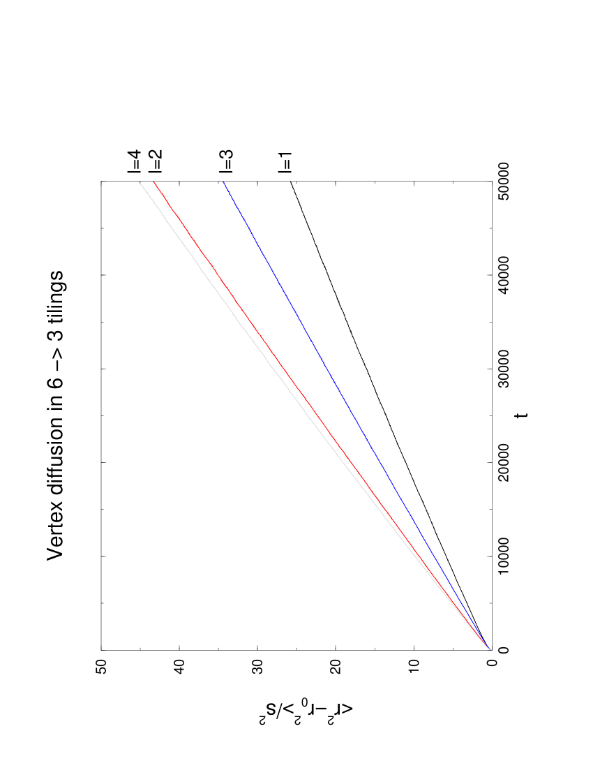
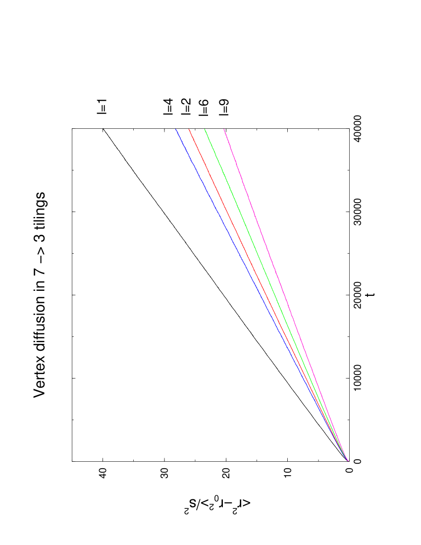
As anticipated from reference [21], this quantity grows like at large time, indicating a diffusive regime, whatever the edge orientation we choose, as displayed in figure 12. We comment these numerical results at the end of the section, after clarifying some technical points.
First of all, the diffusion constant depends not only on the codimension and on the equivalence class of edge orientations, but also on the precise choice of these orientations in a given equivalence class, since there is some liberty of rotating and elongating the vectors in a same class. There is no obvious way in the general case of particularizing a reference orientation in a given class. The only case where it is possible is the first 6-line arrangement, for which edges pointing towards the vertices of a regular icosahedron maximize the symmetry. To smooth the differences between orientation vectors inside an equivalence class, we normalize the mean square displacement by the typical square distance covered by the vertices at each step.
In addition, the mean square displacement exhibits a transition regime before the diffusive one because of short-time correlations. This regime stops around . One can interpret the duration of this transient regime as the typical time between two uncorrelated flips [21]. Indeed, a vertex just being flipped can only be flipped again to its initial position at the next step. To have larger distances covered by a vertex, the flip of this vertex has to be followed by a collective sequence of vertex flips around it. During this sequence, the vertex can go to a new flippable configuration. This collective succession of flips should take a time of order . This time is found to lie between and MCS in all the cases studied here. A vertex can be seen as a standard random walker making independent steps of typical length every MCS and .
The diffusion constants we find after normalization do not depend much on the codimension and the class of edge orientations, which indicates that cycles have no clear influence on vertex diffusion. However, the normalized diffusion constants we find for different edge orientations in a same equivalent class show that this normalization is not sufficient. The order of magnitude of the differences between these diffusion constants in a same equivalence class is of the same order as those between different classes. So we are not able to compare quantitatively the differences in the diffusive dynamics between two classes. However, we can display quantitative results in the case of icosahedral symmetry where orientation vectors are well defined. In this case, we find normal diffusion with a not normalized diffusion constant , which is very close to the one found in reference [21] in the case of periodic-boundary tilings.
But again, the aim of this study was more to observe the possible fundamental differences in flip dynamics between tilings with and without cycles. In particular to check if anomalous diffusion arises in tilings with cycles. The results shown in figure 12 present no anomalous diffusion whatever the tiling problem we are considering. They also show that the diffusion constants are of the same order of magnitude in the three cases: (i) no cycles in any fibration; (ii) cycles in some fibrations but not all of them; (iii) cycles in all fibrations (in which case the connectivity remains open).
As a conclusion, cycles do not seem to have any significant influence on diffusive properties of vertices. We naturally expect that large tilings inherit this diffusive behavior, and that vertices display the same diffusive dynamics in free-boundary tilings related to real quasicrystals, as it is argued in the previous section.
To close this section, we mention that the study of diffusion enables a rough estimate of ergodic times in tiling sets. We recall that the ergodic time of a Markovian process is the typical time the process needs to reach stationarity, in other words to be likely to have reached any configuration with nearly equal probability. A time scale can be associated with vertex diffusion, and is related to the approach of stationarity: it is the typical time needed by a vertex to explore the whole tiling, namely for a tiling of typical radius . This time is compatible with known ergodic times in dimension 2 [34, 26] and in tilings [10]. Since does not depend much on the line arrangement, neither does this typical time .
8 Conclusion and discussion
This paper studies sets of three- (and higher-) dimensional tilings by rhombohedra endowed with local rearrangements of tiles called elementary flips or localized phasons. It uses a coding of tilings by generalized partitions which turns out to be a powerful tool to prove connectivity by flips in a large variety of cases. These results answer positively (even though partially) an old conjecture of Las Vergnas [27]. The general idea of the proof is as follows: consider a tiling problem of codimension . We intend to prove the connectivity of its configuration space . The generalized partition-on-tiling point of view provides a natural decomposition of into disjoint fibers above a base. The base is the configuration space of a tiling problem of codimension . Therefore if it can be proven inductively that the latter configuration space is connected and that all fibers are connected, the overall connectivity of follows.
So far, attempts of proofs of connectivity have failed because of the possible existence of cycles in generalized partition problems. As it is discussed in the paper, these cycles block locally some type of flips, the proof of connectivity of fibers a priori fails and the simple iterative proof of overall connectivity fails in its turn. What we demonstrate in this paper is that this problem can be bypassed in a large majority of cases because, in general, there exists one way of implementing the generalized partition (one “fibration”) so that it does not generate cycles. As a consequence, fibers are connected. Since it can also be proven inductively that the base is connected, the overall connectivity can be established.
We say “a large majority of cases” because the result depends on the choice of edge orientations. Indeed, we address in this paper the implications in random tiling theory and quasicrystal science of this issue. For example, beside the usual orientation of edges associated with the icosahedral symmetry, there exist 3 additional non-equivalent choices of edge orientations for codimension-three tilings. This means that we consider tilings with the same number of different tile species (namely 20), but the 4 sets of tile species are all non-equivalent in that sense that the tilings they generate cannot be put in one-to-one correspondence. It happens that cycles exist only in the icosahedral case but cannot exist in the three remaining cases. As a consequence, the only codimension-three case where we cannot establish connectivity is the icosahedral one. Similarly, there are 11 non-equivalent edge orientations in codimension 4 and we prove connectivity in all of them except 2.
The counterparts of cycles at the tiling level are jammed clusters of tiles that are more difficult to break by flips than the remainder of the tiling because some type of flips is locally absent. It was legitimate to anticipate that they might be responsible for entropic barriers and slow down flip dynamics. We have chosen to address the possible effects of cycles on flip dynamics from the angle of vertex self-diffusion because it is a key issue at the physical level. We prove in this paper that there exist tiling problems of the same codimension with (i) no cycles in any fibration; (ii) cycles in some fibrations but not all of them; (iii) cycles in all fibrations. Connectivity holds in cases (i) and (ii) and remains open in case (iii). We compared self-diffusion in the three cases, and we did not detect any significant effect such as a sub-diffusive regime. Therefore even if cycles break connectivity in case (iii), they do not affect significantly the diffusive properties of physical interest.
The tilings considered here have non-physical fixed boundaries. However, we have argued that a macroscopic central region of tilings is not influenced by the boundary and can therefore be considered as a free-boundary one. This central region contains the jammed clusters of tiles due to cycles. As a consequence, they are not specific to fixed-boundary tilings. We concentrated our attention on this region. We concluded that our results can be transposed to free-boundary random tilings which are more realistic models of quasicrystals.
Beyond diffusive properties, flip dynamics can be characterized by the calculation of ergodic times (the times needed to reach stationarity in the flip Markovian process). We have not addressed this question in the paper. The only conclusion that we can draw is that a diffusive behavior is compatible with ergodic times quadratic in the system size. This point will have to be clarified in the future, but beyond numerical techniques, the methods to tackle this point ought to be invented. The standard methods in this field cannot easily be adapted because of the existence of cycles which make impossible the calculation of these times in fibers that are not connected.
Another issue that is not addressed in this paper is the influence of energy interactions between tiles at finite temperature. More realistic tiling models take into account a tile Hamiltonian (reminiscent of interactions at the atomic level) that favors a quasicrystalline order at low temperature. We intend to analyze the effects of cycles in this context in a future work.
To finish with, we mention that the possible influence of cycles can be quantified on other observables than vertex self-diffusion. For example, we have explored in a preliminary work how the parts converge towards their average value. The part value in the generalized partition formalism is an indication of the position of a tile in the tiling. A deviation in the limiting values would mean that some tiles do not find easily their equilibrium positions in the tiling. It would be a manifestation of ergodicity (or even connectivity) breaking. In general the convergence is rapid. However, we have observed in rare circumstances in the case (iii) above that these values do not converge exactly to their expected equilibrium limit. But in the state of progress of this work, it would be premature to draw any conclusion because we are not able yet to distinguish definitively between a real effect and statistical noise. This work is in progress.
More generally, even if cycles do not perturb the physical properties related to diffusion, we have not excluded the possible occurrence of ergodicity (or even connectivity) breaking due to cycles in icosahedral random tilings, which are related to real quasicrystals. It could have important consequences on physical properties related to flip dynamics but not directly to diffusion, such as relaxation of the structure after a mechanical perturbation (e.g. healing of phason faults behind a dislocation) or a quench. Indeed even if it is always possible to break tiles in a real quasicrystal to bypass a possible locking due to cycles, such a process requires to pass an energy barrier, which might become difficult at low temperature. Moreover, ergodicity breaking would have dramatic consequences in Monte Carlo simulations based on flip dynamics.
Acknowledgments
One of us (ND) is indebted to Victor Reiner for making him aware of the existence of cycles and of non-equivalent edge orientations in dimension 3. We also express our gratitude to Rémy Mosseri, Éric Rémila and Daniel Caillard for fruitful discussions and debates.
Appendix A Connectivity of codimension 1 and 2 tiling sets in any dimension
In this appendix, we prove connectivity of sets of codimension-1 and 2 rhombus tilings of any dimension . In codimension 1, the proof is immediate since such tilings are coded by (acyclic) hyper-solid partitions [15] and since we prove in B that they are consequently connected. In codimension 2, we also use a proof by monotony as in section 5, even if we do not work directly on hyper-plane arrangements in the projective space . Note that all edge orientations are equivalent in any dimension and codimensions 1 and 2 [46].
We code tilings as generalized partitions on codimension-one tilings. For sake of convenience, we identify with the hyperplane of of equation and we choose the vectors as follows:
| (4) | |||||
The -th orientation which orients base tilings is chosen as
| (5) |
where is a small positive parameter. This choice is a convenient one among any (non-degenerate) other one because all edge orientations are equivalent in codimension 2 [46]. A face of a base tiling is oriented accordingly to . Now we exhibit precisely the orientation of each face species.
A face species is defined by edge orientations among the possible ones. We denote by and , , the two indices of the edge orientations that do not define a face species, and by this face species. We also denote by the vector normal to the faces . A simple calculation shows that
| (6) |
where the non-zero coordinates are in positions and . We define when and when . Then for any and : a face is oriented positively in the direction .
In addition, whatever , which proves that and are companion vectors, which in turn proves the monotony of the de Bruijn indices with respect to the order between tiles. The connectivity follows as in section 5.
Appendix B Connectivity of a fiber when the base tiling is acyclic
In this section, we demonstrate that when a base tiling (or more generally a generalized partition problem) is acyclic, the corresponding fiber is connected. We prove that any partition can be connected to the minimum partition where all parts are set to 0.
We proceed by induction on the sum of the parts of . Suppose the result holds for all such that . Consider a partition with .
Among all the parts of bearing non-zero parts, consider a minimal one with respect to the order between parts. Such a part exists because of the acyclic character of the partition problem. Set this part to 0 by successive single flips. The so-obtained partition is connected to because , which proves that is connected by flips to .
References
References
- [1] D. Levine, P.J. Steinhardt, Quasicrystals: a new class of ordered structure, Phys. Rev. Lett. 53, 2477 (1984).
- [2] V. Elser, Comment on “Quasicrystals: a new class of ordered structures”, Phys. Rev. Lett. 54, 1730 (1985).
- [3] C.L. Henley, Random tiling models, in Quasicrystals, the State of the Art, Eds. D.P. Di Vincenzo, P.J. Steinhart (World Scientific, 1991), 429.
- [4] R. Penrose, The role of aesthetics in pure and applied mathematical research, Bull. Inst. Math. Appl. 10, 226 (1974).
- [5] R. Kenyon, Tiling a polygon with parallelograms, Algorithmica 9, 382 (1993).
- [6] S. Elnitsky, Rhombic tilings of polygons and classes of reduced words in Coxeter groups, J. Combinatorial Theory A 77, 193–221 (1997).
- [7] Tilings of zonotopes: Discriminental arrangements, oriented matroids, and enumeration, G.D. Bailey, Ph. D. Thesis (Univ. of Minnesota, 1997).
- [8] H. Cohn, M. Larsen, J. Propp, The shape of a typical boxed plane partition, New York J. of Math. 4, 137 (1998).
- [9] H. Cohn, R. Kenyon, J. Propp, A variational principle for domino tilings, J. of the AMS 14, 297 (2001).
- [10] J. Linde, C. Moore, M.G. Nordahl, An -dimensional generalization of the rhombus tilings, in Proceedings of the Conference DM-CCG: Discrete Models: Combinatorics, Computation, and Geometry (Paris, 2001), p. 23.
- [11] M. Duneau, A. Katz, Quasiperiodic patterns, Phys. Rev. Lett. 54, 2688 (1985); A.P. Kalugin, A.Y. Kitaev and L.S. Levitov, Al0.86Mn0.14: a Six-Dimensional Crystal, JETP Lett. 41, 145 (1985); A.P. Kalugin, A.Y. Kitaev and L.S. Levitov, 6-Dimensional Properties of Al0.86Mn0.14, J. Phys. Lett. France 46, L601 (1985).
- [12] V. Elser, Solution of the dimer problem on a hexagonal lattice with boundary, J. Phys. A: Math. Gen. 17, 1509 (1984).
- [13] R. Mosseri, F. Bailly, C. Sire, Configurational entropy in random tiling models, J. Non-Cryst. Solids, 153&154, 201 (1993).
- [14] R. Mosseri, F. Bailly, Configurational entropy in octagonal tiling models, Int. J. Mod. Phys. B, Vol 7, 6&7, 1427 (1993).
- [15] N. Destainville, R. Mosseri, F. Bailly, Configurational entropy of codimension-one tilings and directed membranes, J. Stat. Phys. 87, 697 (1997).
- [16] N. Destainville, R. Mosseri, F. Bailly, Fixed-boundary octagonal random tilings: a combinatorial approach, J. Stat. Phys. 102, 147 (2001).
- [17] M. Widom, R. Mosseri, N. Destainville, F. Bailly, Arctic octahedron in three-dimensional rhombus tilings and related integer solid partitions, J. Stat. Phys. 109, 945 (2002).
- [18] Regular Polytopes, H.S.M. Coxeter (Dover, 1973).
- [19] L.-H. Tang, Random-tiling quasicrystal in three dimensions, Phys. Rev. Lett. 64, 2390 (1990).
- [20] L.J. Shaw, V. Elser, C.L. Henley, Long-range order in a three-dimensional random-tiling quasicrystal, Phys. Rev. B 43, 3423 (1991).
- [21] M.V. Jarić, E. Sørensen, Self-diffusion in random-tiling quasicrystals, Phys. Rev. Lett. 73, 2464 (1994).
- [22] F. Gälher, in Proceedings of the fifth international conference on quasicrystals, Eds. C. Janot and R. Mosseri (World Scientific, Singapore, 1995), p. 236.
- [23] W. Ebinger, J. Roth, H.R. Trebin, Properties of random tilings in three dimensions, Phys. Rev. B 58, 8338 (1998).
- [24] P.A. Kalugin, A. Katz, A mechanism for self-diffusion in quasi-crystals, Europhys. Lett. 21 (9), 921 (1993).
- [25] M. Wollgarten, M. Beyss, K. Urban, H. Liebertz, U. Köster, Direct evidence for plastic deformation of quasicrystals by means of a dislocation mechanism, Phys. rev. Lett. 71, 549 (1993).
- [26] N. Destainville, Flip dynamics in octagonal rhombus tiling sets, Phys. Rev. Lett. 88, 30601 (2002).
- [27] M. Las Vergnas, Convexity in oriented matroids, J. Comb. Theory Ser. B 29, 231 (1980).
- [28] V. Reiner, The generalized Baues problem, in New Perpspectives in Geometric Combinatorics, Eds. L.J. Billera, A. Björner, C. Greene, R.E. Simion, R.P. Stanley, MSRI publications 38, Cambridge University Press, 293 (1999).
- [29] N.G. de Bruijn, Algebraic theory of Penrose’s non-periodic tilings of the plane, Kon. Nederl. Akad. Wetensch. Proc. Ser. A 84 (1981) 1-38.
- [30] N.G. de Bruijn, Dualization of multigrids, J. Phys. France 47 (1986) C3-9.
- [31] Oriented matroids, A. Björner, M. Las Vergnas, B. Sturmfels, N. White, G.M. Ziegler (Cambridge University Press, 1993).
- [32] B. Sturmfels, G.M. Ziegler, Extention spaces of oriented matroids, Discrete & Computational Geom. 10, 23 (1993).
- [33] K.J. Strandburg, P.R. Dressel, Thermodynamic behavior of a Penrose-tiling quasicrystal, Phys. Rev. B 41, 2469 (1990).
- [34] D. Randall and P. Tetali, Analyzing Glauber dynamics by comparison of Markov chains, J. Math. Phys. 41 (3), 1598 (2000).
- [35] Lectures on Polytopes, G.M. Ziegler (Springer-Verlag, 1995).
- [36] Convex Polytopes, B. Grünbaum (Interscience Publishers, 1967).
- [37] F. Chavanon, E. Rémila, Rhombus tilings: decomposition and space structure, preprint, Tech. report of ENS Lyon, RR2004-30 (2004).
- [38] Introduction to Lattices and Order, 2nd edition, B. A. Davey, H. A. Priestley (Cambridge University Press, 2002).
- [39] G. Coddens, C. Soustelle, R. Bellissent, Y. Calverac, Study of hopping in perfect icosahedral AlFeCu quasi-crystal by inelastic neutron scattering, Europhys. Lett. 23, 33 (1993).
- [40] S. Lyonnard, G. Coddens, Y. Calvayrac, D. Gratias, Atomic (phason) hopping in perfect icosahedral quasicrystals Al70.3 Pd21.4 Mn8.3 by time-of-flight quasielastic neutron scattering, Phys. Rev. B 53, 3150 (1996).
- [41] R. Blüher, P. Scharwaechter, W. Frank, H. Kronmüller, First low-temperature radiotracer studies of diffusion in icosahedral quasicrystals, Phys. Rev. Lett. 80, 1014 (1998).
- [42] K. Urban, M. Feuerbacher, M. Wollgarten, M. Bartsch, U. Messerschmidt, in Physical Properties of Quasicrystals, Ed. Z.M. Stadnik, Solid State Science 126, Springer, 361 (1999).
- [43] D. Caillard, F. Mompiou, private communication (2004).
- [44] D. Caillard, F. Mompiou, L. Bresson, D. Gratias, Dislocation climb in icosahedral quasicrystals, Scripta Mater., 49, 11 (2003).
- [45] F. Mompiou, L. Bresson, P. Cordier, D. Caillard, Dislocation climb and low-temperature plasticity of an Al-Pd-Mn quasicrystal, Phil. Mag. 83, 3133 (2003).
- [46] E. Rémila, private communication (2003). The proof is based upon an argument of duality in the context of oriented matroid theory that is beyond the scope of this paper.