Unzipping of DNA with correlated base-sequence.

Abstract

We consider force-induced unzipping transition for a heterogeneous DNA model with a correlated base-sequence. Both finite-range and long-range correlated situations are considered. It is shown that finite-range correlations increase stability of DNA with respect to the external unzipping force. Due to long-range correlations the number of unzipped base-pairs displays two widely different scenarios depending on the details of the base-sequence: either there is no unzipping phase-transition at all, or the transition is realized via a sequence of jumps with magnitude comparable to the size of the system. Both scenarios are different from the behavior of the average number of unzipped base-pairs (non-self-averaging). The results can be relevant for explaining the biological purpose of correlated structures in DNA.

I Introduction.

Structural transformations of DNA under changing of external conditions are of importance for molecular biology bio and biophysics biofiz . They take place in transcription of genetic information from DNA and in duplication of DNA during cell division bio . The common scenario of these processes is unwinding of the double-stranded structure of DNA under influence of external forces. Recall that a deoxyribonucleic acid (DNA) consists of two strands with one winded around the other. These two strands interact via hydrogen bonds due to which the double-helix structure is formed. The individual strand is constructed by covalent bonds whose strength is thus much larger than the inter-strand coupling. Each strand is a polymer based on nucleotides. A nucleotide is a deoxyribose sugar molecule bearing on one side purine or pyrimidine group (the base) and on the other a phosphate group. The purines can be of two type: adenine (A) and guanine (G), whereas pyrimidines are cytosine (C) and thymine (T) (an additional purine uracil (U) is found in ribonucleic acid (RNA)). A, G, C and T groups differentiate the nucleotides and constitute the genetic code carried by a DNA molecule. The bounds between neighboring nucleotides within one strand are formed via the corresponding phosphate groups. Hydrogen bonds between opposite strands are formed either by A-T bases or by G-C bases. Since the bases A, G, C and T are hydrophobic, they are located at the core of the double-helix. In contrast, the sugar molecules and the phosphate groups are hydrophilic and they are located in the outside part of the DNA molecule. Thus in a regular DNA molecule the letters of the genetic code are hidden from the molecular environment. This appears as a problem for the polymerase enzymes whose role is to read the genetic code. The polymerase may function if only they unzip the needed part of the DNA molecule, so that the bases are exposed to the environment. This is the main reason why DNA unzipping, in particular, unzipping under an external force is important for functioning of all living organisms. Force-induced unzipping has been actively investigated only recently  hindu ; non-hindu ; maritan ; nelson ; exp motivated by the new generation of micromanipulation experiments  exp ; expreview .

It is expected that features of the unzipping process depend on the base-sequence of DNA, because AT and GC base-pairs do have different formation energies. It is more difficult to break a single GC base-pair, since it is made of three hydrogen bonds, while a single AT base-pair is made of two hydrogen bonds only. Thus, the formation energy difference between AT and GC base-pairs is of the order of one hydrogen bond energy, that is, $0.1-0.2$ eV. This is comparable with the average formation energy itself. We note in addition that for a given DNA molecule the overall concentrations of AT and GC base-pairs are approximately equal bio . This is especially true for higher organisms, e.g., the concentration of GC base-pairs for primates is between 49 and 51% bio .

The above energy difference may not be relevant for certain bulk properties of DNA. Therefore, the latter is frequently modeled assuming a homogeneous base-sequence. However, in natural conditions the energy supplied for uzipping can be comparable to the average formation energy, and then the heterogeneous character of the base-sequence becomes relevant. One of the first steps in this direction was made in nelson , where it was shown that short-range heterogenity does influence the unzipping process in the region where the energy supplied by an external unzipping force is comparable to the average formation energy of a DNA base-pair.

Our main purpose is to make the next step towards real DNAs and to analyze force-induced unzipping for a DNA-model, where the structural features of the base-sequence are taken into account. One of the known features of DNA is that its base-sequence displays substantial correlations which, in particular, can be of long-range characters longrange ; voss ; coding ; review : two base pairs separated from each other by thousands of pairs appear to be statistically correlated. Initial studies reported long-range correlations for non-coding regions of DNA (introns). For higher organisms, e.g. humans, these regions constitute more than 90% of DNA bio . It was believed for some time that coding regions, which carry the majority of genetic information, can have only short-range correlations. However, more recent results indicate on the existence of weak long-range correlations in coding regions as well coding (this point was controversial for a while, but the general consensus on its validity emerged gradually). Moreover, systematic changes were found in the structure of correlations depending on the evolutionary category of the DNA carrier voss . In spite of ubiquity of long-range correlations, their biological reason remains largely unexplored. Some attempts in this direction were made in  jenya , where it was studied why long-range correlations are absent in certain biologically active proteins.

Our basic purpose in the present paper will be to determine how statistical correlations, in particular long-range correlations, influence on the unzipping process. Due to the biological relevance of unzipping, indications of such influences can provide useful information for explaining the presence of long-range correlations in DNA.

This paper is organized as follows. The basic model we work with is described in section II. The situation with finite-range correlated base-sequence is investigated in section III.1. The next three sections study various aspects of the long-range correlated situation. We conclude with a summary of our results. Several technical points are outlined in appendices.

II The model

There are three basic mechanisms which determine the physics of the unzipping process: An external force tending to unbind the double-helix structure of a DNA molecule, thermal noise generated by an equilibrium environment into which the molecule is embedded, and finally structural features of the molecule itself. Among various structural features which may be of relevance, the most important ones are connected with the base-sequence of the molecule.

We shall work with a model which takes into account these three physical ingredients in the most minimal way. It was recently proposed in Ref. nelson for studying DNA unzipping.

i) A DNA molecule is lying along the $x$-axis between the points $x=a$ and $x=L$.

ii) Among all degrees of freedom of the molecule we consider only base-pairs; they are located at points $x_{i}$, $a<x_{i}<L$, $i=1,...,M$. Indeed, for that range of external force where the molecule is close to be unbind completely, those degrees of freedom which are related to hydrogen bonds have much shorter characteristic times as compared to other degrees of freedom. The latter ones can therefore be considered as adiabatically frozen, and excluded from the effective description we are developing.

iii) Any base-pair can be in one of two states: bound or disconnected (broken). We choose the overall energy scale in such a way that the latter case contributes to the Hamiltonian a binding energy $\phi(x_{i})$, whereas the former case brings nothing. As we stressed in the introduction, different types of base-pairs do have different binding energies: even when considering the ideal situation, where there are no “wrong base-pairs” such as AC and GT, the “correct” base-pairs AT and GC are different with respect to energy needed to unbind them. Thus $\phi(x_{i})$ is a random quantity with an average $\langle\phi\rangle$:

$$\phi(x_{i})=\langle\phi\rangle+\eta(x_{i}).$$ (1)

iv) An external force is acting on the left end $x=a$ of the molecule pulling apart the two strands. Thus, if a bond $x_{i}$ is broken, all the base-pairs $x_{j}$ with $j<i$ are broken as well. Each broken bond brings additionally to the Hamiltonian a term $-{\cal F}$, where ${\cal F}$ is proportional to the acting force.

v) Summarizing all of these, one comes to the Hamiltonian

$$H(x)=-{\cal F}x+\sum_{i=1}^{x}\phi(x_{i})=(\langle\phi\rangle-{\cal F})x+\sum_{i=1}^{x}\eta(x_{i}),$$ (2)

where $x$ is the number of broken base-pairs.

In the thermodynamical limit, where $L,M\gg 1$, one applies the continiuum description with $x$ being a real number, $a<x<L$, and ends up with the following Hamiltonian:

$$H(x)=(x-a)\,f+\int_{a}^{x}{\rm d}s\,\eta(s),$$ (3)

where $f=\langle\phi\rangle-{\cal F}$ and $\beta=1/T$ is the inverse temperature ($k_{\rm B}=1$).

vi) For characteristic time-scales of unzipping experiments we can certainly neglect any changes of the base-sequence for a single DNA molecule. Thus, once it is modeled via the random noise $\eta$, it is legitimate to assume that this noise is frozen, i.e. its single realization corresponds to a single molecule. It is assumed that the DNA molecule is embedded into a thermal bath with temperature $T$, and had sufficient time to reach equilibrium. Thus, the partition function and the free energy corresponding to the Hamiltonian (3) read:

$$Z=\int_{a}^{L}{\rm d}x\,e^{-\beta H(x)},\qquad F=-T\ln Z.$$ (4)

These quantities are still random together with $\eta$. Average results of many experiments with various realizations of $\eta$ can be described with help of the average free energy $\langle F\rangle$. Our order parameter is the number of broken base-pairs $X$. Along with its average it is defined for $t=0$ as

$$X=\partial_{f}F,\quad\langle X\rangle=\partial_{f}\langle F\rangle.$$ (5)

II.1 Finite-range and long-range correlated situations.

vi) It remains to specify the properties of the noise $\eta$. Within the adopted description we assume it is a Gaussian stationary process with an autocorrelation function

$$K(t-t^{\prime})=\langle\eta(t)\eta(t^{\prime})\rangle,\qquad K(t)=K(-t).$$ (6)

Two major classes can now be distinguished depending on the behavior of $K(t)$ for large $t$. The finite-range correlated situation is defined by requiring that the integral

$$D=\int_{0}^{\infty}{\rm d}s\,K(s),$$ (7)

determining the total intensity of the noise is finite. There are three particular case of the finite-range correlated situation. The white noise case,

$$K(t)=D\delta(t),$$ (8)

describes completely uncorrelated noise. The physical situation given by (3, 8) is well known, and was used to describe interfaces, random walks in a disordered media, and population dynamics manfred . It was recently applied for the unzipping transition in DNA nelson . Similar models were considered in maritan ; azbel .

The second case corresponds to the noise having some finite — though possibly large — correlation length $\tau$. The simplest and most widely used model for this case is provided by Ornstein-Uhlenbeck (OU) noise

$$K(t)=\frac{D}{\tau}\,e^{-|t|/\tau},$$ (9)

where $D$ is the total intensity of the noise, and $\tau$ is the correlation time; $\tau\to 0$ corresponds to the white noise. The third case is when $K(t)$ has a power-law dependence for large $t$, but still decays sufficiently quickly so that the integral in (7) is finite: $K(t)\propto|t|^{-\delta}$ with $\delta>1$.

The second major class is the long-range correlated situation, where the integral in (7) is infinite, that is when $K(t)$ for sufficiently large $t$ behaves according to a power law voss :

$$K(t)\equiv\langle\eta(t)\eta(0)\rangle=\sigma|t|^{-\alpha},$$ (10)

where

$$0<\alpha<1$$ (11)

is the exponent characterizing the long-range correlation, and where $\sigma$ is the (local) intensity. Note that $K(t)$ has to be regular and finite for small $t$ review , as one would expect from physical reasons.

The OU noise (9), as the typical representative of the finite-range correlated situation, and the long-range correlated noise (10) are relevant for modeling correlations in base-sequence of DNA longrange ; voss ; coding ; review ; maria . Note, however, that the real noise distributions in DNA can be much more complicated voss ; coding . In particular, this concerns the Gaussian property we assume (see in this context section V.1, where we study a model of a non-Gaussian noise to show that its predictions in the thermodynamic limit do not differ from those given by the corresponding Gaussian noise). For the long range correlated situation there can exist several characteristic exponents for different ranges of $t$. Nevertheless, Eqs. (9, 10) are certainly the minimal models of noise which are sufficiently simple and which allow to study both finite and long range correlations.

II.2 Reduction to Langevin equation.

The basic method of solving the present model will be to reduce it to the physics of a Brownian particle whose dynamics is described by a stochastic differential equation. In Eq. (4) one fixes $L$, and views $a$ as a parameter varying from the highest possible value $L$, where $Z=0$, to the lowest possible value which we define to be $a=0$. The quantity $t=-a$ will thus monotonicaly increase and can be interpreted as a time-variable. Differentiating $Z$ in (4) over $a$ and changing the variable as $t=-a$, one gets:

$$\frac{{\rm d}Z}{{\rm d}t}=1-\beta fZ-\beta\,\eta(t)Z,\qquad-L<t<0$$ (12)

where we used $\eta(t)=\eta(-t)$, as follows from the Gaussian stationary property of the noise. This is a Langevin equation with a multiplicative noise. From (12) one can obtain a stochastic equation for $F=-T\ln Z$:

$$\frac{{\rm d}F}{{\rm d}t}+V^{\prime}(F)=\eta(t),\quad V(F)=T^{2}e^{\beta F}-fF.$$ (13)

This is the basic stochastic equation we will work with.

III Finite range correlated noise.

III.1 Ornstein-Uhlenbeck noise.

Our main purpose here is to study the process of unzipping in the presence of the finite range corelated noise given by Eq. (9). We wish to understand how the magnitude of $\tau$ influences unzipping.

Note that the OU noise (9) can itself be modeled via a white-noise:

$$\tau\,\dot{\eta}=-\eta+\sqrt{D}\,\xi(t),$$ (14)

where $\xi(t)$ is a Gaussian noise with delta-correlated spectrum:

$$\langle\,\xi(t)\xi(t^{\prime})\,\rangle=2\delta(t-t^{\prime}).$$ (15)

Indeed, Eq. (9) is recovered directly from (14, 15), since their exact solution is:

$$\langle\,\eta(t)\eta(t^{\prime})\,\rangle=e^{-(t+t^{\prime})/\tau}\left(\langle\,\eta^{2}(0)\,\rangle-\frac{D}{\tau}\right)+\frac{D}{\tau}\,e^{-|t-t^{\prime}|/\tau}.$$ (16)

We get back from here Eq. (9) under an additional consistency condition $\langle\,\eta^{2}(0)\,\rangle={D}/{\tau}$. Moreover, $\eta(t)$ is Gaussian random process, because $\xi(t)$ is Gaussian and Eq. (14) is linear risken .

To handle (13) one differentiates it over $t$ and uses (14, 15). Changing the variable as $s=t/\sqrt{\tau}$ one gets hanggi :

$$\frac{{\rm d}^{2}F}{{\rm d}s^{2}}+\gamma(F)\,\frac{{\rm d}F}{{\rm d}s}=-V^{\prime}(F)+\frac{\sqrt{D}}{\tau^{1/4}}\xi(s),$$ (17)

where

$$\gamma(F)=\tau^{-1/2}+V^{\prime\prime}(F)\,\tau^{1/2}.$$ (18)

Eq. (17) has the same form as a Langevin equation for a particle with unit mass in the potential $V(F)$ and subjected to a white noise and a $F$-dependent friction with a coeffcient $\gamma(F)$. Note that the potential $V(F)$ is confining only for $f>0$: $V(F)\to\infty$ for $F\to\pm\infty$.

We can rewrite Eq. (17) introducing an additional variable $\widetilde{F}(s)={{\rm d}F(s)}/{{\rm d}s}$, which in the above language of the Brownian motion corresponds to the velocity.

$$\frac{{\rm d}F}{{\rm d}s}=\widetilde{F},$$ (19)

$$\frac{{\rm d}\widetilde{F}}{{\rm d}s}=-\gamma(F)\,\widetilde{F}-V^{\prime}(F)+\frac{\sqrt{D}}{\tau^{1/4}}\xi(s).$$ (20)

As $\xi(t)$ is a Gaussian white noise, one uses the standard tools, see e.g. risken , and writes down from (19, 20) a Fokker-Planck-Klein-Kramers equation for the common probability distribution:

$$P(F,\widetilde{F},s)=\langle\,\delta(F-F(s))\,\delta(\widetilde{F}-\widetilde{F}(s))\,\rangle,$$ (21)

where $F(s)$ and $\widetilde{F}(s)$ are particular noise-dependent solutions of (19, 20), and where the average is taken over the white noise $\xi(t)$ given by Eq. (15).

$$\frac{\partial P(F,\widetilde{F},s)}{\partial s}=-\widetilde{F}\,\frac{\partial P(F,\widetilde{F},s)}{\partial F}+\gamma(F)\,\frac{\partial[\,\widetilde{F}\,P(F,\widetilde{F},s)\,]}{\partial\widetilde{F}}+V^{\prime}(F)\,\frac{\partial P(F,\widetilde{F},s)}{\partial\widetilde{F}}+\frac{D}{\tau^{1/2}}\,\frac{\partial P(F,\widetilde{F},s)}{\partial\widetilde{F}^{2}}.$$ (22)

Our interest is in the large-$s$ limit of this equation (thermodynamic limit), and we want to have the reduced probability distribution $P(F,s)$ of $F$ only:

$$P(F,s)=\langle\,\delta(F-F(s))\,\rangle=\int{\rm d}\widetilde{F}\,P(F,\widetilde{F},s).$$ (23)

To this end let us introduce

$$Q_{n}(F,s)=\int{\rm d}\widetilde{F}\,\widetilde{F}^{n}\,P(F,\widetilde{F},s)\qquad n=0,1,2,3..,$$ (24)

where $Q_{0}(s)=P(F,s)$. From (22) one gets an infinite set of coupled equations for $Q_{n}(F,s)$:

$$\frac{\partial Q_{0}(F,s)}{\partial s}=-\frac{\partial Q_{1}(F,s)}{\partial F},$$ (25)

$$\frac{\partial Q_{1}(F,s)}{\partial s}=-\frac{\partial Q_{2}(F,s)}{\partial F}-\gamma(F)\,Q_{1}(F,s)-V^{\prime}(F)\,Q_{0}(F,s),$$ (26)

$$\frac{\partial Q_{2}(F,s)}{\partial s}=-\frac{\partial Q_{3}(F,s)}{\partial F}-2V^{\prime}(F)\,Q_{1}(F,s)-2\gamma(F)\,Q_{2}(F,s)+\frac{2D}{\tau^{1/2}}\,Q_{0}(F,s),$$ (27)

$$......$$ (28)

When deriving (25–26) we used integration by parts, and the following standard boundary conditions:

$$P(F,\widetilde{F},s)\to 0,\quad{\rm if}\quad F\to\pm\infty,\quad{\rm or}\qquad{\rm if}\quad\widetilde{F}\to\pm\infty.$$ (29)

These conditions are physically meaningful if the potential $V(F)$ is confining, and thus the motion of the corresponding Brownian particle takes place in a finite domain. According to the above discussion on the confining character of the potential $V(F)=T^{2}e^{\beta F}-fF$, the boundary conditions (29) are reliable only for $f>0$.

Recall that the “time-variable” $t$ moves between $-|L|$ and $0$. For large lengths, i.e. for $L\gg 1$ (thermodynamic limit) and as the consequence $t\propto s\to 0$, any solution of the equation (22) relaxes towards the unique stationary distribution $P_{\rm st}(F,\widetilde{F})$. A rather general proof of this fact is presented in risken .

We shall now use (25–26) to get explicitly the stationary distribution function $P_{\rm st}(F)$ of $F$. Putting to zero the LHS of (25) one gets that $Q_{1,{\rm st}}(F)$ does not depend on $F$. Taking into account the boundary condition (29) one concludes that it is equal to zero:

$$Q_{1,{\rm st}}(F)=0.$$ (30)

Putting to zero the LHS of (26) and using (30) we get

$$\frac{\partial Q_{2,{\rm st}}(F)}{\partial F}=-V^{\prime}(F)\,Q_{0,{\rm st}}(F).$$ (31)

It remains to determine $Q_{2,{\rm st}}(F)$ putting to zero the LHS of Eq. (27). One can conjecture that the stationary state $P_{\rm st}(F,\widetilde{F})$ is symmetric with respect to $\widetilde{F}\to-\widetilde{F}$, and then $Q_{3,{\rm st}}(F)=0$ in the same way as for $Q_{1,{\rm st}}(F)$ in (30). Alternatively, one can assume that $\gamma(F)$ and $D$ are sufficiently large so that the term $\partial Q_{3,{\rm st}}(F)/\partial F$ can be simply dropped in the RHS of (27). If $V^{\prime\prime}(F)$ is of order one, then a large $\gamma(F)$ is realized both for large and small $\tau$ hanggi . Thus we conclude from (27):

$$\gamma(F)\,Q_{2,{\rm st}}(F)=\frac{D}{\tau^{1/2}}\,Q_{0,{\rm st}}(F).$$ (32)

In view of (31, 32) one has a single differential equation:

$$\frac{D}{\sqrt{\tau}}\,\frac{\partial}{\partial F}\left(\frac{Q_{0,{\rm st}}(F)}{\gamma(F)}\right)=-V^{\prime}(F)\,Q_{0,{\rm st}}(F),$$ (33)

and gets for $Q_{0,{\rm st}}(F)\equiv P_{\rm st}(F)$,

$$P_{\rm st}(F) \propto\,\gamma(F)\exp\left[-\frac{\tau}{2D}[V^{\prime}(F)]^{2}-\frac{1}{D}V(F)\right],$$

$$P_{\rm st}(F) =\,{\cal N}(1+\tau\,e^{\beta F})\exp\left[\frac{fF}{D}-\frac{T\left(T-\tau f\right)e^{\beta F}}{D}-\frac{\tau T^{2}}{2D}\,e^{2\beta F}\,\right].$$ (34)

where ${\cal N}$ is the normalization factor. The white-noise, $\tau\to 0$, limit of $P_{\rm st}(F)$ was obtained in Refs. manfred ; nelson .

Figure 1: $\langle X\rangle$ for Ornstein-Uhlenbeck noise with $D=10$, $T=1$. From right to left: $\tau=0$, $\tau=10$, $\tau=100$. It is seen that, for a fixed $f$, $\langle X\rangle$ decreases upon increasing $\tau$.

According to (5, 34) the average free energy reads:

$$\langle F\rangle=T\,\frac{\int_{0}^{\infty}{\rm d}u\,\ln(u)\left(\tau+\frac{1}{u}\right)\,u^{\mu}\,\exp\left[\left(\mu\tau-\frac{T^{2}}{D}\right)\,u-\frac{\tau T^{2}}{2D}\,u^{2}\right]}{\int_{0}^{\infty}{\rm d}u\left(\tau+\frac{1}{u}\right)\,u^{\mu}\,\exp\left[\left(\mu\tau-\frac{T^{2}}{D}\right)\,u-\frac{\tau T^{2}}{2D}\,u^{2}\right]},$$ (35)

where

$$\mu=\frac{Tf}{D}.$$ (36)

Note that both integrals in (35) can be expressed through the gamma-function $\Gamma(x)$ and the confluent hypergeometric (Kummer) function ${}_{1}F_{1}(a,b;z)$, since

$$\int_{0}^{\infty}{\rm d}u\,u^{c}\,e^{au^{2}-bu}=\frac{1}{2}\,a^{-1-c/2}\,\Gamma\left(1+\frac{c}{2}\right)\left[b~{}_{1}F_{1}\left(1+\frac{c}{2},\frac{3}{2},\frac{b^{2}}{4a}\right)+\sqrt{a}~{}_{1}F_{1}\left(\frac{1+c}{2},\frac{1}{2},\frac{b^{2}}{4a}\right)\right].$$ (37)

Similar formulas can be written for $\int_{0}^{\infty}{\rm d}u\,u^{c}\,(\,\ln u\,)^{n}\,e^{au^{2}-bu}$ for $n=1,2$. These representations facilitate numerical calculations.

The average number of broken base-pairs $\langle X\rangle$ can be calculated from (5, 34). Note that for the white-noise situation $\tau\to 0$ a simple formula is obtained:

$$\langle X\rangle=\frac{T^{2}}{D}\,\frac{{\rm d}\psi(\mu)}{{\rm d}\mu},$$ (38)

where $\psi(\mu)=\Gamma(\mu)/\Gamma^{\prime}(\mu)$. For $\mu\to 0$, $\langle X\rangle$ does not depend on temperature and on $\tau$ and becomes very large:

$$\langle X\rangle=D\,f^{-2},$$ (39)

for $f\to 0$. When the external force reaches its critical value, the average number of broken base-pairs diverges in the thermodynamic limit.

To study the influence of $\tau$ on this unzipping phase transition, one should keep in mind the realistic situation, where DNA molecules belonging to different evolutionary classes have different correlation properties of their base-sequences voss . At the same time the concentration (fraction) of AT and GC base-pairs is known to be (approximately) equal for sufficiently long DNA molecules in natural conditions bio ; f1 . Therefore, in comparing two situations having different correlation characteristics, it is legitimate to keep fixed the intensity of the noise defined by Eq. (7) — this corresponds to fixed concentration of various base-pairs — and to study how the average number of broken base-pairs $\langle X\rangle$ depends on $\tau$ for some fixed value of $f$. This dependence is displayed in Fig. (1) following to Eqs. (5, 35). It is seen that the behavior of $\langle X\rangle$ for very small $f$ depends on $\tau$ rather weakly. Indeed, as follows from Eq. (34), for $f\to 0$ the relevant domain of $F$ contributing into $\langle F\rangle$ is $F\sim-D/f$. As it does not depend on $\tau$, we get back Eq. (39). However, a non-trivial dependence on $\tau$ does exist for moderately small values of $f$, where as seen in Fig. 1, $\langle X\rangle$ is a decreasing function of $\tau$ for a fixed $f$: longer correlations present in the base-sequence increase the stability of the DNA molecule, since larger external forces ${\cal F}$ needed to achieve the same average amount of broken base-pairs. This is our main qualitative conclusion on how a finite correlation length influences the unzipping process.

III.2 Arbitrary finite-range correlated noise at low temperatures.

In the previous section we reduced the non-linear equation (13) with the finite range correlated noise (9) to a Fokker-Planck equation, and solved the latter exactly in the thermodynamic limit. The essential feature that made this analytical solution possible is that the OU noise has a single and well-defined characteristic time and due to this allows representation (14, 15).

In general it is impossible to solve (13) for an arbitrary Gaussian noise, and, in particular, for the situation given by Eq. (10): there is no exact Fokker-Planck equation for this case. There is, however, a particular case which allows analytical treatment. For very low temperatures, $T\to 0$, one can approximately substitute $V(F)$ in Eq. (13) by $-fF$ for $F<0$ and by an infinite potential wall standing at $F=0$. Thus, all values $F>0$ become prohibited. For this particular form of potential one can get a Fokker-Planck equation for

$$P(F,t)=\langle\delta(F-F[\eta,t])\rangle$$ (40)

with an arbitrary Gaussian noise in the RHS of Eq. (13). The derivation goes as follows. Write Eq. (13) as

$$\frac{{\rm d}F}{{\rm d}t}=f+\eta(t),$$ (41)

where the stochastic variable $F$ is restricted to be negative due to the above infinite wall. Differentiating $P(F,t)$ in (40) over $t$ one gets

$$\frac{\partial P(F,t)}{\partial t}=-f\,\frac{\partial P(F,t)}{\partial F}-\frac{\partial}{\partial F}\,\langle\eta(t)\,\delta(F-F[\eta,t])\rangle.$$ (42)

It remains to handle the last term in this equation. One uses Novikov’s theorem fox

$$\langle\eta(t)\,\delta(F-F[\eta,t])\,\rangle=-\frac{\partial}{\partial F}\int_{-L}^{t}{\rm d}s\,K(t-s)\left\langle\,\delta(F-F[\eta,t])\,\frac{\delta F[t]}{\delta\eta(s)}\,\right\rangle,$$ (43)

where $\delta\,/\delta\eta(s)$ is the variational derivative and $\delta F[t]/\delta\eta(s)$ is obtained from (41):

$$\frac{{\rm d}}{{\rm d}t}\frac{\delta F[t]}{\delta\eta(s)}=\delta(t-s),\qquad\frac{\delta F[t]}{\delta\eta(s)}=\theta(t-s),$$ (44)

where $\theta(t-s)$ is the step function. Combining (42, 43, 44) we get finally

$$\frac{\partial P(F,t)}{\partial t}=-f\,\frac{\partial P(F,t)}{\partial F}+D_{t}\frac{\partial^{2}P(F,t)}{\partial F^{2}},$$ (45)

$$D_{t}=\int_{0}^{t+L}{\rm d}s\,K(s).$$ (46)

Eq. (45) should additionally be supplemented by a boundary condition which reflects the presence of the infinite wall at $F=0$. Equation (45) can be written as the continuity equation

$$\frac{\partial P(F,t)}{\partial t}+\frac{\partial J(F,t)}{\partial F}=0,\qquad J(F,t)=f-\mu_{t}\frac{\partial P(F,t)}{\partial F},$$ (47)

where $J(F,t)$ is the probability current. The infinite wall at $F=0$ is now implemented by requiring:

$$\int_{-\infty}^{0}{\rm d}F\,P(F,t)=1,$$ (48)

$$J(0,t)=0,$$ (49)

for all $t$. Conditions (48, 49) are imposed on any solution of (45).

In the thermodynamic limit $L\to\infty$ and $t=0$ one gets from the stationarity condition ${\partial P(F,t)}/{\partial t}=0$

$$P(F)= \frac{f}{D}\,\exp\left[\frac{fF}{D}\right],\qquad{\rm for}\qquad F<0,$$ (50)

$$= 0,\qquad\qquad\qquad\quad{\rm for}\qquad F\geq 0,$$ (51)

where the total intensity, as given by (7), is finite for the considered short-range correlated situation. Note that in the thermodynamical limit conditions (48, 49) are satisfied automatically as seen from Eqs. (50, 51). It is now seen from (5) that

$$\langle X\rangle=Df^{-2},$$ (52)

which has the same $f$-dependence as the white-noise case for small $f$; see (39). We conclude that, not unexpectedly, for low temperatures the behavior of $X$ is determined only the total intensity of the noise. All other details of $K(t)$ do not matter. It remains to stress that the present analysis certainly does not apply to the long-range correlated situation (10), since the total intensity $D$ diverges in the thermodynamical limit.

In closing this section, let us note that Eq. (52) can be applied to finite-range correlated noise that for $t\ll L$ has the same autocorrelation function as (10). As an example take

$$K_{\rm fr}(t)= \sigma|t|^{-\alpha},\quad{\rm for}\quad|t|\leq l,$$ (53)

$$= 0,\qquad\quad{\rm for}\quad|t|>l,$$ (54)

where $l$ is some parameter that is finite in the thermodynamical limit $L\to\infty$. Therefore, the noise given by Eq. (53) is obviously finite-range correlated. Eq. (52) now reads

$$\langle X\rangle=\frac{\sigma}{1-\alpha}\,l^{1-\alpha}\,f^{-2}.$$ (55)

If one chooses to take $l\sim\langle X\rangle$ then $\langle X\rangle\sim f^{-2/\alpha}$ as predicted in Ref. nelson . However, there is no any a priori reason for this choice, and at any rate this result refers to the finite-range correlated noise $K_{\rm fr}$. The real long-range correlated situation, where $l\sim L$, is still not described by it.

IV Long-range correlated situation: the frozen noise limit.

The present and the next section are devoted to the long-range correlated situation, where according to Eq. (10) the autocorrelation function $K(t)$ of the noise has a power-law behavior with the single characteristic exponent $1>\alpha>0$.

To start with, let us consider the case with $\alpha\to 0$. The noise is now completely frozen: $\eta(s)$ in (3) does not depend on $s$. This situation is less physical as compared to that with $\alpha>0$. However, it is exactly solvable, and one can hope it catches at least some features of the realistic situation where $\alpha$ is larger than zero, but certainly smaller than one. This intuitive expectation will be confirmed later on.

The problem with $\alpha=0$ is easily solved from (3). Moreover, the exact solution can be obtained for an arbitrary value of $L$:

$$\frac{X}{L}=g[\,\beta L(f+\eta)\,],$$ (56)

$$g[x]\equiv\frac{1}{x}-\frac{1}{e^{x}-1}.$$ (57)

It is seen that in the thermodynamical limit $L\to\infty$, $g[\,\beta L(f+\eta)\,]$ behaves as roughly the step-function, $g[\,\beta L(f+\eta)\,]\simeq\theta(-\eta-f)$: for any single realization of the noise there is a sharp phase transition with a jump at the realization-dependent point $f=-\eta$. Exactly at this point $f=-\eta$ one has $g(0)=1/2$ and $\langle X\rangle=L/2$.

Let us now study the behavior of $\langle X\rangle$. Since the noise is completely frozen, the calculation of $\langle X\rangle$ reduces to the averaging over a Gaussian variable with dispersion $\sigma$. We have

$$\frac{\langle X\rangle}{L}=\left\langle\,g[\,\beta L(f+\eta)\,]\,\right\rangle\equiv\int\frac{{\rm d}\eta}{\sqrt{2\pi\sigma}}\,\exp\left[-\frac{\eta^{2}}{2\sigma}\right]\,g[\,\beta L(f+\eta)\,]=\int\frac{{\rm d}\xi}{\sqrt{2\pi\sigma\beta^{2}}}\,\exp\left[-\frac{(\xi-\beta f)^{2}}{2\sigma\beta^{2}}\right]g[\,L\xi\,],$$ (58)

where we changed the integration variable as $\xi=\beta(\eta+f)$. In the thermodynamical limit $L\to\infty$, we shall obtain for $\langle X\rangle/L$ the main term of order ${\cal O}(L^{0})$, and the first correction to it which will appear to be of order ${\cal O}(1/L)$. To this end, let us divide the integration in the RHS of (58) into three pieces:

$$\int=\int_{-\infty}^{-2/L}+\int_{-2/L}^{2/L}+\int_{2/L}^{\infty}.$$ (59)

For each piece we shall use the following aproximate expressions obtained from (58)

$$g[\,L\xi\,] =\frac{1}{L\,\xi},\qquad{\rm for}\qquad L\,\xi\gtrsim 2,$$ (60)

$$g[\,L\xi\,] =\frac{1}{2},\qquad\qquad{\rm for}\qquad-2\lesssim L\,\xi\lesssim 2,$$ (61)

$$g[\,L\xi\,] =1+\frac{1}{L\,\xi},\quad\qquad{\rm for}\qquad L\,\xi\lesssim-2.$$ (62)

To obtain (60) and (62) we neglected terms of order ${\cal O}(e^{-\beta L|f|})$ that is certainly legitimate in the thermodynamic limit. For (61) which corresponds to the second integration piece in (59), we have taken the value of $g[\,L\xi\,]$ at $\xi=0$. The boundary points of $L\xi$ were chosen such as to ensure a continuous matching. However, neither the precise value of $g[\,L\xi\,]$ within the second piece of integration in (59), nor the precise values of the points separating this piece from the remaining ones are important, since as we show below the contribution coming from this second piece, as well as the contributions from the boundary points of the two other integration pieces, produce factors of order ${\cal O}(1/L^{2})$ at best.

Combining (60–62) with (58) one gets

$$\frac{\langle X\rangle}{L} =\int_{-\infty}^{-2/L}\frac{{\rm d}\xi}{\sqrt{2\pi\sigma\beta^{2}}}\,\exp\left[-\frac{(\xi-\beta f)^{2}}{2\sigma\beta^{2}}\right]\left(1+\frac{1}{L\xi}\right)+\frac{1}{2}\int_{-2/L}^{2/L}\frac{{\rm d}\xi}{\sqrt{2\pi\sigma\beta^{2}}}\,\exp\left[-\frac{(\xi-\beta f)^{2}}{2\sigma\beta^{2}}\right]$$ (66)

$$+\int_{2/L}^{\infty}\frac{{\rm d}\xi}{\sqrt{2\pi\sigma\beta^{2}}}\,\exp\left[-\frac{(\xi-\beta f)^{2}}{2\sigma\beta^{2}}\right]\,\frac{1}{L\xi}$$

$$=\int_{-\infty}^{0}\frac{{\rm d}\xi}{\sqrt{2\pi\sigma\beta^{2}}}\,\exp\left[-\frac{(\xi-\beta f)^{2}}{2\sigma\beta^{2}}\right]+\frac{1}{L}\int_{0}^{\infty}\frac{{\rm d}\xi}{\xi\sqrt{2\pi\sigma\beta^{2}}}\left(\exp\left[-\frac{(\xi-\beta f)^{2}}{2\sigma\beta^{2}}\right]-\exp\left[-\frac{(\xi+\beta f)^{2}}{2\sigma\beta^{2}}\right]\right)$$

$$-\frac{1}{L}\int_{0}^{2/L}\frac{{\rm d}\xi}{\xi\sqrt{2\pi\sigma\beta^{2}}}\left(\exp\left[-\frac{(\xi-\beta f)^{2}}{2\sigma\beta^{2}}\right]-\exp\left[-\frac{(\xi+\beta f)^{2}}{2\sigma\beta^{2}}\right]\right)$$

$$+\frac{1}{2}\int_{0}^{2/L}\frac{{\rm d}\xi}{\sqrt{2\pi\sigma\beta^{2}}}\left(\exp\left[-\frac{(\xi-\beta f)^{2}}{2\sigma\beta^{2}}\right]-\exp\left[-\frac{(\xi+\beta f)^{2}}{2\sigma\beta^{2}}\right]\right).$$

One notes that both (66) and (66) are of order ${\cal O}(1/L^{2})$. This can be verified by directly expanding integrals in (66) and (66) for small $2/L$. Skipping these terms, one gets

$$\frac{\langle X\rangle}{L} =\int_{\beta f}^{\infty}\frac{{\rm d}\xi}{\sqrt{2\pi\sigma\beta^{2}}}\,\exp\left[-\frac{\xi^{2}}{2\sigma\beta^{2}}\right]+\frac{1}{L}\int_{0}^{\infty}\frac{{\rm d}\xi}{\xi\,\sqrt{2\pi\sigma\beta^{2}}}\,\left(\exp\left[-\frac{(\xi-\beta f)^{2}}{2\sigma\beta^{2}}\right]-\exp\left[-\frac{(\xi+\beta f)^{2}}{2\sigma\beta^{2}}\right]\right)$$ (67)

$$=\int_{\beta f}^{\infty}\frac{{\rm d}\xi}{\sqrt{2\pi\sigma\beta^{2}}}\,\exp\left[-\frac{\xi^{2}}{2\sigma\beta^{2}}\right]+\frac{1}{\sigma\beta^{2}L}\exp\left[-\frac{f^{2}}{2\sigma}\right]\int_{0}^{\beta f}{\rm d}\xi\,\exp\left[\frac{\xi^{2}}{2\sigma\beta^{2}}\right],$$

When obtaining the last term in the RHS of (67), we used a tabulated identity for the error function.

For $f$ not very large as compared to $\sqrt{\sigma}$, the first term in the LHS of (67) is dominating: ${\langle X\rangle}/{L}$ is or order one-half. In particular, it is exactly equal to one-half for $f=0$. The dependence of $\langle X\rangle$ on $f$ becomes thus very weak for $f\to 0$. The second, subdominant term become non-negligible for $f\gg\sqrt{\sigma}$, where using asymptotic identities (see Appendix B):

$$\int_{a}^{\infty}\frac{{\rm d}\xi}{\sqrt{2\pi}}\,e^{-\xi^{2}/2}=\frac{e^{-a^{2}/2}}{a\sqrt{2\pi}}\,\left(1-\frac{1}{a^{2}}+\dots\right),\qquad a\gg 1,$$ (68)

$$\int_{0}^{a}{{\rm d}\xi}\,e^{\xi^{2}/2}=\int_{0}^{a}{{\rm d}\xi}\,e^{\xi^{2}/2}=\frac{e^{a^{2}/2}}{a}\left(1+\frac{1}{a^{2}}\right)+\dots,\qquad a\gg 1,$$ (69)

one gets from (67) noting $a=f/\sqrt{\sigma}$:

$${\langle X\rangle}=\frac{1}{\beta f}\left(1+\frac{\sigma}{f^{2}}+\frac{\sqrt{\sigma}}{\sqrt{2\pi}}\,L\beta\,\exp\left[-\frac{f^{2}}{2\sigma}\right]\right).$$ (70)

Note that for $f\gg\sqrt{\sigma}$, $\langle X\rangle$ has — within the leading order — the same $1/f$-dependence as it will be in the completely homogeneous situation without noise ($\sigma=0$). In the considered regime, the noise only renormalizes this behavior modifying the subdominant terms.

As compared to $X/L$ which has a jump at a realization dependent point $f=\eta$, ${\langle X\rangle}/{L}$ is seen to behave smoothly. It displays a crossover between small $\langle X\rangle/L$ for a large $f$ and $\langle X\rangle=L/2$ for $f=0$: the sharp transition disappears; see Fig. 2. This indicates that the situation for the totally-correlated noise is essentially non-self-averaging: in the thermodynamical limit the averaged order parameter $\langle X\rangle$ does not reproduce the behavior of $X$ for a typical realization. Recall that for disordered systems all observables like free energy, order parameters, correlation functions, etc., depend on the realization of the disorder, i.e. they are random quantities. It is of the immediate interest to know their most probable (typical) values, since they will be met in experiments. If for a given quantity its typical value in the thermodynamic limit coincides with its average, one speaks on self-averaging; see e.g. brout ; de . In practice this means that it is sufficient to study averages as they are representative in the single sample measurements. It is known on the general ground that in the proper thermodynamic limit, that is when the linear size $L$ of the system is much larger than any other characteristic length and provided the distribution of the disorder is finite-range correlated, quantities that scale with the volume of the studied random system — these are extensive quantities such as free energy, order parameter, but not the statistical sum — are expected to display self-averaging brout ; de . This result is based on the law of large numbers. However, this need not be true if the distribution of the disorder is long-range correlated, since now the correlation length of the disorder has the same order of magnitude as the linear size, and the arguments based on the law of large numbers do not apply. The above situation is just of this sort.

IV.1 Dispersion as a measure of non-self-averaging.

It is desirable to have more quantitative indications of the above indicated non-self-averaging effect. To characterize fluctuations of $X$ from one realization to another, it is natural to employ the corresponding dispersion $\langle X^{2}\rangle-\langle X\rangle^{2}$ which tells us how the quantity $\langle X\rangle$ fluctuates from one realization to another. Then the statement of self-averaging will read:

$$\frac{\langle X^{2}\rangle-\langle X\rangle^{2}}{\langle X\rangle^{2}}\to 0,\qquad{\rm for}\qquad L\to\infty.$$ (71)

In contrast, if ${(\langle X^{2}\rangle-\langle X\rangle^{2})}/{\langle X\rangle^{2}}$ remains finite for $L\to\infty$, we have non-self-averaging.

The quantity $\langle X^{2}\rangle$ can be calculated in the same way as in Eqs. (66, 67). We shall bring the result only for $f$ not very large as compared to $\sqrt{\sigma}$, that is, when $\langle X^{2}\rangle\propto L^{2}$:

$$\frac{\langle X^{2}\rangle}{L^{2}}=\int_{\beta f}^{\infty}\frac{{\rm d}\xi}{\sqrt{2\pi\sigma\beta^{2}}}\,\exp\left[-\frac{\xi^{2}}{2\sigma\beta^{2}}\right]+\frac{2}{L}\,\ln\left(\frac{L}{2}\right)\,~{}\frac{\exp\left[-\frac{f^{2}}{2\sigma}\right]}{\sqrt{2\pi\beta^{2}\sigma}}+{\cal O}\left(\frac{1}{L}\right).$$ (72)

Substituting this into (71), we see that ${(\langle X^{2}\rangle-\langle X\rangle^{2})}/{\langle X\rangle^{2}}$ remains finite in the thermodynamical limit:

$$\frac{\langle X^{2}\rangle-\langle X\rangle^{2}}{\langle X\rangle^{2}}=\frac{\int_{\beta f}^{\infty}\frac{{\rm d}\xi}{\sqrt{2\pi\sigma\beta^{2}}}\,\exp\left[-\frac{\xi^{2}}{2\sigma\beta^{2}}\right]}{\left(\int_{\beta f}^{\infty}\frac{{\rm d}\xi}{\sqrt{2\pi\sigma\beta^{2}}}\,\exp\left[-\frac{\xi^{2}}{2\sigma\beta^{2}}\right]\right)^{2}}\,-\,1.$$ (73)

In particular, for $f\to 0$

$$\frac{\langle X^{2}\rangle-\langle X\rangle^{2}}{\langle X\rangle^{2}}\to 1,$$ (74)

indicating essential non-self-averaging.

In closing this section, let us repeat that the character of the thermodynamical for the considered case $\alpha=0$ is different from that of the finite-range correlation situation, where — for $L\to\infty$ — the behavior of $\langle X\rangle$ become independent on $L$ at least in the physical range of other parameters (e.g., $1>f>0$, $T>0$, etc). For the $\alpha=0$ case, as seen from Eqs. (67, 70), there is an explicit dependence on $L$ in the whole range of physical range of the involved parameters. According to (70), if $L$ is kept large but finite, then this dependence is very weak for external forces far form their critical value $f=0$, that is, for $f\gg\sqrt{\sigma}$. There are no reasons for taking this explicit dependence on $L$ as something unphysical. In contrast, the actual size of physically relevant examples of DNA is never more that $L\sim 10^{4}-10^{6}$; see Ref. bio . This is certainly much smaller than the number $10^{23}$ which in the standard statistical physics is taken as the typical size. Therefore, it is rather natural to study the physics of unzipping for a large but fixed $L$.

For the considered frozen situation, we could solve the problem analytically for a given realization. However, for $\alpha>0$ this is not possible, and one has to rely on numerical methods. This is what we intend to do in the next section.

Figure 2: $X(f)/L$ for a particular realization (solid curve) and $\langle\,X(f)\,\rangle/N$ (dotted curve) versus $f$; $T=\sigma=1$, and $L=10^{4}$.

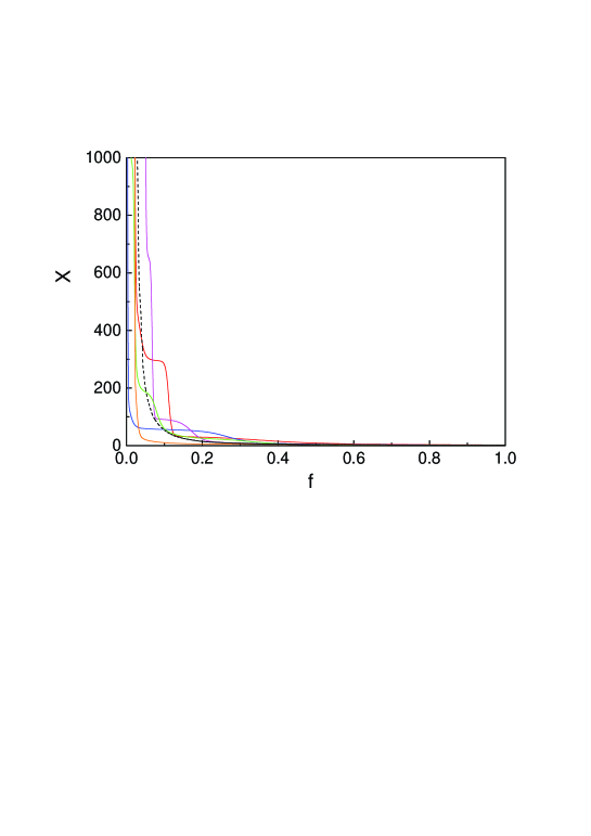
Figure 3: Solid curves: $X(f)$ for several realizations of the white uncorrelated noise. Dotted curve: $\langle X(f)\rangle$ obtained by averaging over $10^{3}$ realizations. $T=D=1$, $L=5\times 10^{4}$.

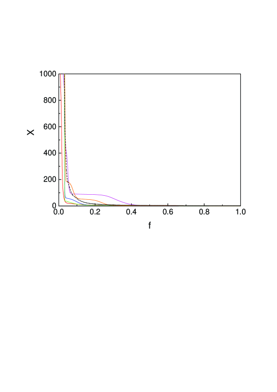
Figure 4: Solid curves: $X(f)$ for several realizations of the dichotomic uncorrelated noise ($\eta_{i}=\pm 1$ with equal probability). Dotted curve: $\langle X(f)\rangle$ obtained by averaging over $10^{3}$ realizations. $T=1$, $L=5\times 10^{4}$.

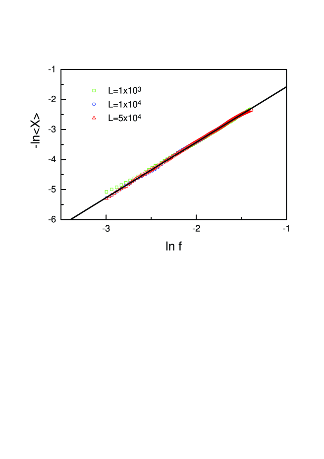
Figure 5: The dependence of $-\ln\langle X(f)\rangle$ on $\ln f$ for various values of $L$ and for $T=D=1$. The quantity $\langle X(f)\rangle$ was obtained by direct averaging over $10^{3}$ realizations. Solid line idicates linear fitting $-\ln\langle X(f)\rangle=A+1.84179\,\ln f$ for $L=5\times 10^{4}$, where $A$ is a constant. The emergence of the power-law (76) is thus displayed explicitly.

V Numerical results.

As we have seen in the previous section, there are reasons to expect that for the long-range correlated situation, especially for sufficiently small index $\alpha$, the typical — that is, frequently met among many independent realizations of the noise — behavior of $X(f)$ in the thermodynamic limit is not described adequately by the average quantity $\langle X\rangle$ (non-self-averaging). We note in this context that the correlator $(\langle X^{2}\rangle-\langle X\rangle^{2})/{\langle X\rangle^{2}}$ studied in section IV can indicate on non-self-averaging, but by itself does not provide any direct information on typical realizations. It is perhaps needless to stress that once we expect the effect of non-self-averaging, the attention should be shifted towards typical realizations, since they do have a direct physical meaning for single-molecule experiments.

In the present section we study numerically the behavior of the number of broken base-pairs $X$ as a function of $f$ both for the long-range correlated situation and for the uncorrelated noise. For the discrete version of the model the partition function reads:

$$Z=\sum_{k=1}^{L}\exp[-\beta(fk+\sum_{i=1}^{k}\eta_{i})],$$ (75)

where for the long-range correlated situation $\eta_{i}$ are Gaussian random variables with the autocorrelation function given by (10). Note that for the purposes of numerical computations the behavior of $K(t)$ in (10) was regularized at short distances so as to avoid superfluous short-range singularities; see Appendix A for details. The generation of $\eta_{i}$, $i=1,...,L$ is described in Appendix A following to optimized recipes proposed in sancho . For numerical computations we have chosen $T=1$ and $L=10^{4}$ or $L=5\times 10^{4}$.

As $L$ is now explicitly finite, one should be careful with the selection of the thermodynamical domain, since due to the very statement of the problem the limit $L\to\infty$ is taken before $f\to 0$. As a plausible estimate of this domain, one can use a condition $f\sqrt{L}\gg 1$. We confirmed it in several ways, reproducing predictions which were made in the thermodynamica limit $L\to\infty$.

V.1 Uncorrelated noise.

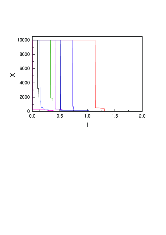
Figure 6: Realizations of $X(f)$ from the first class of typicality. $T=\sigma=2\alpha=1$, $L=10^{4}$.

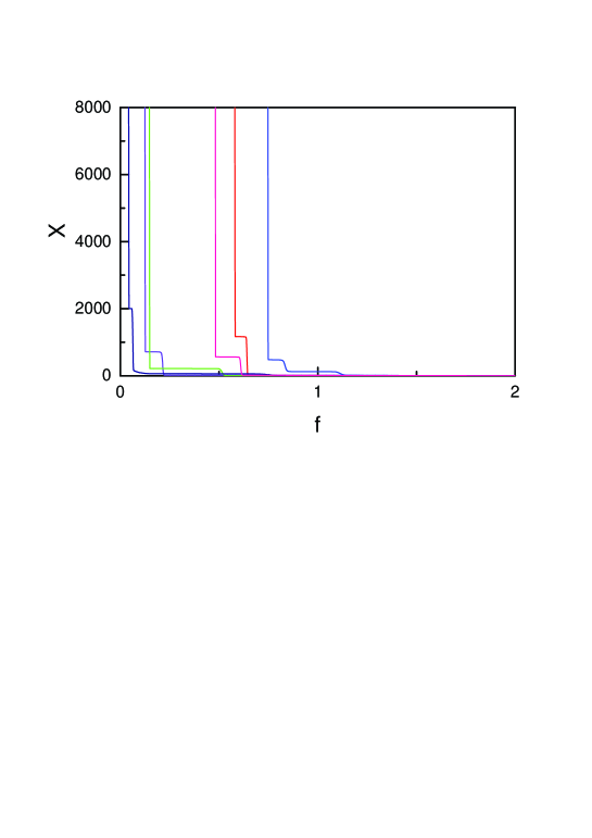
Figure 7: Realizations of $X(f)$ from the first class of typicality. $T=\sigma=2\alpha=1$, $L=5\times 10^{4}$.

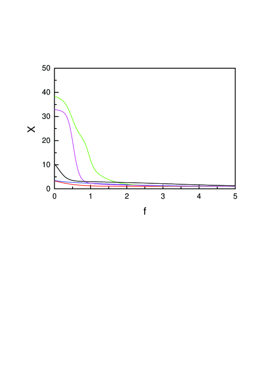
Figure 8: Realizations of $X(f)$ from the second class of typicality. $T=\sigma=2\alpha=1$, $L=10^{4}$.

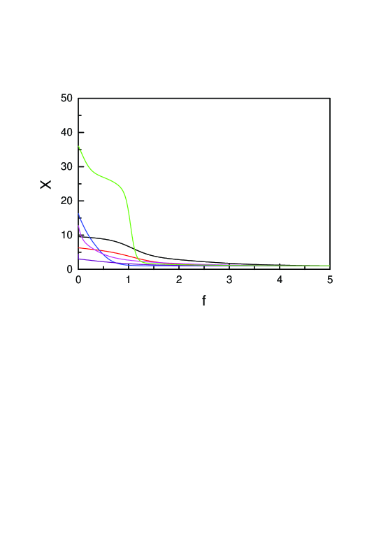
Figure 9: Realizations of $X(f)$ from the second class of typicality. $T=\sigma=2\alpha=1$, $L=5\times 10^{4}$.

Let us start with the uncorrelated noise case, where $\eta_{i}$’s are independent Gaussian variables with zero average, $\langle\eta_{i}\rangle=0$, and variance $\langle\eta^{2}_{i}\rangle=D=1$ (white noise), and where $X$ is given by (5, 75). For comparison we also studied a case, where $\eta_{i}$ are independent random variables assuming values $\eta_{i}=\pm 1$ with equal probability (dichotomic noise).

The results are illustrated by Figs. (3, 4), where we display $\langle X\rangle$ and $X$ for several typical realizations. It is seen that $\langle X\rangle$ and $X$ do not coincide exactly, as it is in general expected due to the finite magnitude of $L$ if not by any other reason. However, in the considered thermodynamical domain of $f$ the behavior of various typical realizations qualitatively resembles each other, and, therefore, resembles that of $\langle X(f)\rangle$. In particular, for all typical realizations $X(f)$ grows for $f\to 0$. In that sense $f=0$ is a special point for both typical $X$ and $\langle X\rangle$. It should be mentioned that for $f\leq 0.05$ we have seen realizations containing relatively sudden jumps at realization-dependent values of $f$. This differs from the behavior of $\langle X\rangle$ and is in agreement with results of Ref. nelson . However, such small values of $f$ are not in the thermodynamical domain. Acknowledging reservations connected with the numerical character of our study, we, nevertheless, conclude that the uncorrelated-noise situation is self-averaging at least for not very small, $f\sqrt{L}\gg 1$, values of $f$.

It is seen from Fig. (4) that the white and dichotomic noise produce very similar results. This is to be expected for the considered large values of $L$ (law of large numbers). Fig. (5) shows that the power law $\langle X\rangle\propto f^{-2}$ for the white-noise case is recovered by direct averaging over various realizations. Indeed, it is seen from this figure that one recovers

$$\langle X\rangle\propto f^{-1.84},$$ (76)

after averaging over $10^{3}$ realizations in the domain $0.05<f<0.25$. This result is stable upon increasing the number of realizations, e.g. from $10^{3}$ to $2\times 10^{3}$.

V.2 Long-range correlated noise

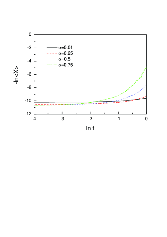
Figure 10: $-\ln\langle X\rangle$ versus $\ln f$ for the long-range correlated noise with various $\alpha$’s and $L=5\times 10^{4}$, $T=\sigma=1$. The quantity $\langle X(f)\rangle$ was obtained by direct averaging over $10^{3}$ realizations.

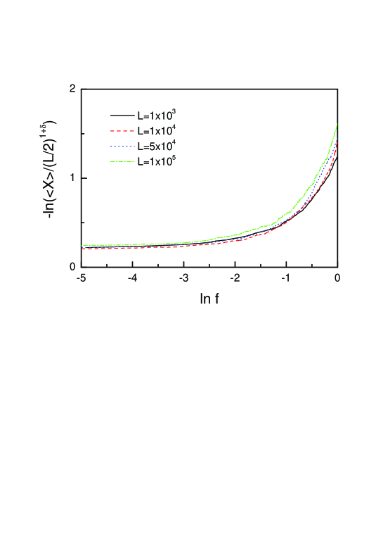
Figure 11: $-\ln\left(\langle X\rangle\,(L/2)^{-1-\delta(\alpha)}\right)$ versus $\ln f$ for various $L$’s and $T=\sigma=1$, $\alpha=0.25$, $\delta=0.0625$. The quantity $\langle X(f)\rangle$ was obtained by direct averaging over $10^{3}$ realizations.

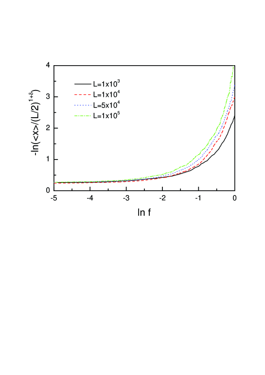
Figure 12: The same as in Fig. (11) but with $\alpha=0.5$ and $\delta=0.075$.

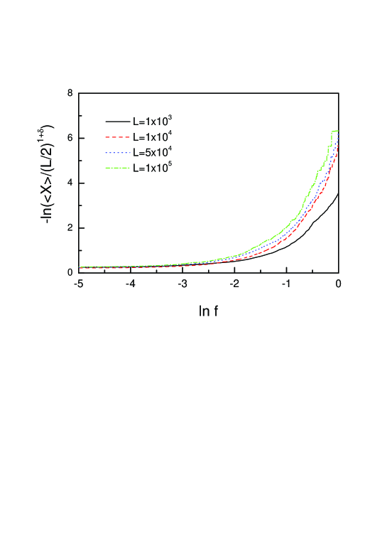
Figure 13: The same as in Fig. (11) but with $\alpha=0.75$ and $\delta=0.08$.

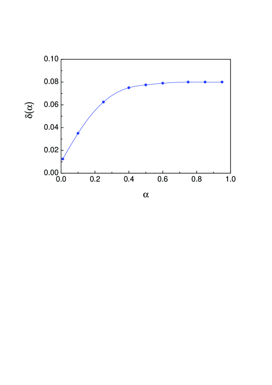
Figure 14: $\delta(\alpha)$ defined by Eq. (78) versus $\alpha$.

V.2.1 Typical realizations.

The situation for the long-range correlated noise for $\alpha=0.5$, $T=\sigma=1$ is illustrated by Figs. (6, 8, 7, 9). The first point to note is that now there are typical realizations with radically different properties. The first type of realizations is presented by Figs. (6, 7): $X(f)$ increases by several sudden jumps followed by flat regions. It is seen that $X|_{f=0}$ is either equal to its maximal possible value $L$ or is close to it. Points where $X(f)$ has jumps vary from one realization to another. However, the overall number of jumps when varying $f$ between zero and one is typically two or three.

In contrast to this, Figs. (8, 9) presents a strictly different situation: It is characterized by very smooth behavior of $X(f)$ for $f\geq 0$. In particular, $X|_{f=0}$ is much smaller than $L$ (typically by few orders of magnitude). $X(f)$ is still a monotonic function of $f$, but the point $f=0$ — where the energy supplied by the external unzipping force is equal to the average binding energy of a base-pair — is by no means special.

To estimate the frequency by which each scenario is met among all possible realizations, we have taken the following criteria for deciding whether a given realization belongs to one of the above classes: for $L=5\times 10^{4}$ we prescribe the given realization to the first class if $X(f=0)>4.8\times 10^{4}$, while it is prescribed to the second class if $X(f=0)<10^{2}$. These criteria appeared to be sufficiently adequate, as they are consistent with the fact of presence (for the first class) of absence (for the second class) of sudden jumps for $X(f)$.

In this way the frequencies of each class were estimated in a sample of $10^{3}$ realizations. It appeared for $L=5\times 10^{4}$ and $T=\sigma=2\alpha=1$ that the first scenario is met in $\sim 84\%$ of all cases ($839$ in $10^{3}$ realizations), while the second scenario is present in $\sim 12\%$ of all cases ($118$ in $10^{3}$ realizations). These fractions are stable upon increasng the size of the sample on which the above estimation were carried out. Interestingly enough, realizations where $X(f)$ as a function of $f$ fall into neither of the above two classes amount only to $\sim 4\%$ of all possible cases.

It is relevant to note that the fractions of the two classes show tendency to move towards each other upon decreasing the size of the system. For instance, the fractions of the first and the second class amount to $18\%$ and $76\%$, respectively, for $L=10^{4}$ ($T=\sigma=2\alpha=1$). These fractions were estimated by criteria $X(f=0)>0.8\times 10^{4}$ and $X(f=0)<10^{2}$, respectively. Recall in this context that the chosen values for $L$ are sensible, since the typical DNA samples used in experiment have $L\sim 10^{4}-10^{5}$; see, e.g., bio ; biofiz and also section V.2.2.

Since there are typical realizations which are so much different from each other, we conclude that this long-range situation is essentially non-self-averaging in the whole physical domain $0<f<1$ and, in particular, in the thermodynamical domain of $f$. This fact distinguishes between the uncorrelated (white noise) and long-range correlated situations. It should be noted that due to the law of large numbers any non-self-averaging present in the whole domain $0<f<1$ is certainly impossible for the uncorrelated (or weakly correlated) noise brout ; de . For the long-range correlated case the very law of large numbers does not apply, and the above effect becomes possible.

Our discussion of the frozen noise presented in section IV allows to provide a qualitative explanation for features of the above two classes of typical realizations. One notes that a sizeable portion of long-range correlated noise realizations can be seen as several pieces of the frozen noise with different $\eta$’s put next to each other. Now recall from (56) that every sufficiently long piece of that type has a single first order phase transition with a jump proportional to its length.

The same reasoning can be applied for the understanding of the existence of the second class, where $X(f)$ is a smooth function of $f$ and $X(f=0)\ll L$. Here one should note that — within the above qualitative image of a long-range correlated random sequence — there are realizations of the noise where all $\eta$’s are positive, and thus all jumps of $X(f)$ can occur only for negative $f<0$, that is, beyond the domain of our interest.

V.2.2 Inferring phase transitions.

Let us finally discuss on whether we can infer phase transitions by studying the typical realizations. First of all, it is obvious that once we do not have self-averaging, phase transitions should be studied on typical scenarios of behavior for $X$ and not on the behavior of its average $\langle X\rangle$. There is another aspect which is certainly more subtle: phase transitions are typically defined in the thermodynamical limit and one needs special tools of finite-size scaling for their identification in results of numerical computations which are necessarily done on finite systems. The idea of the finite-size scaling is thus to extrapolate these results to the thermodynamical limit. However, there is another, somewhat different line of thought gross which identifies the proper thermodynamical quantities (such as entropy, free energy, order parameter, etc) directly for finite systems, and then searches in the space of parameters some points having a special character for this quantities. This approach well-recommended itself for studying phase transitions in atomic and nuclear physics, and in systems with long-range interactions (e.g., a gas of self-gravitating particles). For the present study of DNA there is a related aspect that should be taken into account: in natural conditions the number of base-pairs is large, but finite. Here $L$ is of order of $10^{4}\sim 10^{5}$, see e.g. bio ; biofiz , as we have mentioned already. It is, therefore, clear that the considered finite size aspect of DNA is something generic, and not only connected with natural limitations of numerical methods.

Let us now return to the situation presented in Figs. (8, 7, 9). We are going to use the analogy with the case of the totally correlated noise described in section IV. It was seen already that this analogy helped us to draw useful qualitative conclusions on the numerical data. For the totaly correlated noise the point of the phase transition is anambiguously identified with the realization dependent value $f=-\eta$. At this point the order parameter $X$ has a jump of order $L$; see Eqs. (56, 57). It may be useful to repeat that the most unusual aspect of this phase-transition is that its point is strictly realization-dependent. The same philosophy can now be applied to Figs. (6, 7): there are realization-dependent values of $f$, where $X$ has jumps of order of $L/2$ (recall that for the figures we have taken $L=10^{4}$ or $L=5\times 10^{4}$). It is seen as well that there can be several such phase-transitions for a single system (single realization of noise). The latter fact can by itself appear to be rather surprising. However, it is known that some disordered de , or deterministic but strongly-frustrated saqo , systems can experience several phase transitions; there can even exist quasi-continuous domains of criticality saqo . With the same logic one sees that the typical realizations presented in Figs. (8, 9) do not have phase transitions in the domain $0<f<1$ at least for the considered values of $L$.

V.3 The behavior of $\langle X\rangle$.

As we already noted, once the effect of non-self-averaging is present, the basic physical quantities are the typical realizations, since it is these features that are directly observed in experiments. It is, however, still of relevance to know the behavior of the average number of unzipped bonds $\langle X\rangle$, since it illustrates what are the precise differences as compared to typical realizations.

Here we report on two features of $\langle X\rangle$ as a function of $f$. The first one is how does $\langle X\rangle$ depend on $f$ for small values of $f$. In particular, is there any power law dependence similar to $\langle X(f)\rangle\propto f^{-2}$ present in the uncorrelated noise situation, and verified by us numerically in section V.1? Note that for the long-range correlated situation with the index $\alpha$ such a power law

$$\langle X\rangle\propto f^{-2/\alpha},$$ (77)

was recently predicted for small $f$; see Ref. nelson . The most adequate way to look for the power-laws is to plot $-\ln\langle X\rangle$ as a function of $\ln f$, then a power-law should display itself via a straight line. Fig. (10) display such a plot obtained for various values of $\alpha$ and $L=5\times 10^{4}$. The quantity $\langle X\rangle$ was calculated by direct averaging over $10^{3}$ realizations and the results were checked for stability upon increasing (by two times) the number of realizations. As seen, this figure shows very weak dependence of $-\ln\langle X\rangle$ on $\ln f$. There are no convincing indications of a power law. In particular, when decreasing $\alpha$ the dependence of $-\ln\langle X\rangle$ on $\ln f$ does become weaker, in obvious contrast with the prediction made by Eq. (77). For $\alpha\to 0$ this behavior coincides with those of the exact solution discussed in section IV.

It should be noted that $-\ln\langle X\rangle$ is a perfectly smooth function of $\ln f$: all jumps and flat regions present for the first class of typical realizations — which involves the majority of realizations — became washed out when averaging over $10^{3}$ realizations. This gives another indication that the point of jumps in the above class are completely random and vary from one realization to another.

Once we realized that in a rather wide interval of $f$’s — typically $\ln f<-0.5$, as seen in Fig. (10) — the dependence of $\langle X\rangle$ on $f$ is weak, we have studied the behavior of $\langle X(f=0)\rangle$ as a function of $L$ and $\alpha$. As shown by Figs. (11, 12, 13) numerical results fit well into the following scaling equation:

$$\langle X(f\to 0)\rangle\propto\left(\frac{L}{2}\right)^{1+\delta(\alpha)}.$$ (78)

The values of $\delta(\alpha)$ for several $\alpha$’s are shown by Fig. (14). For $\alpha\approx 0$, we get $\delta=0.01$ which is in a good agreement with exact value $\delta(\alpha=0)=0$ got in section IV.

Two important features of result (78) are to be mentioned. First, as seen from Figs. (11, 12, 13) the value of $\langle X\rangle(f=0)$ adequately characterizes the whole domain of small $f$, since the dependence of $\langle X\rangle$ on $f$ is weak. Second, as seen from Fig. (14), the function $\delta(\alpha)$ increases with $\alpha$, but saturates for $\alpha\geq 0.5$ at $\delta=0.08$. It appears that the same result (78) with the index $\delta=0.08$ holds for the uncorrelated noise, but there its region of validity is restricted (for $L=5\times 10^{4}$, $T=\Delta=1$) by very small $f<0.01$ values of $f$, in contrast to the long-range situation. Thus, as far as the small-$f$ characteristics are concerned the result (78) seems to be universal, and it is likely that $\delta(\alpha)$ can have the same status as critical indices in the usual theory of phase transitions.

We conclude by repeating two main qualitative features of the average number $\langle X(f)\rangle$ of unzipped bonds as revealed by our numerical analysis: in the long-range situation and for small forces $f$, the behavior of $\langle X(f)\rangle$ as a function of $f$ does not display any power-law, and is governed by its value at $f=0$. The latter one satisfies to power-law (78) as a function of $L$.

VI Summary and conclusion.

In the present paper we have studied how statistical correlations present in the base-sequence of a DNA molecule influence the process of unzipping. There were two related motivations for our study. On the one hand, the existence of these correlations — that can have both finite-range and long-range character — is by now a well-established fact longrange ; voss ; coding ; review . It is, therefore, legitimate to study how they influence on the DNA physics. On the other hand, general qualitative predicitions drawn on the above influence can be used for explaininig the reason of rich correlated structures found in the base-sequence of DNA. Recall that various segments of a DNA molecule can have different — finite-range or long-range coding ; review — correlation structures. Moreover, DNA molecules belonging to different evolutionary classes have different correlation properties of their base-sequences voss .

The model we studied contains only the most minimal number of ingredients needed to describe unzipping, and to account for correlations in the base-sequence of DNA. Therefore, many realisitic features of the unzipping process remain beyond of our study. We, nevertheless, believe that the obtained results will be useful especially for drawing qualitative conclusions.

Let us now shortly summarize our results starting from the finite-range correlated situation. In section III.1 we have shown that the presence of a finite correlation length $\tau$ plays a stabilizing role for the unziping process: for a fixed external force $f$ the average number of broken base-pairs decreases under increasing of $\tau$. If only finite-range correlations are present, the process of unzipping does not depend much on the detailed structure of the base-sequence: all typical — i.e., frequently met among all possible base-sequeces — scenarios of unzipping have the same qualitative pattern of behavior, that is, the number of the broken base-pairs diverges as the external force approaches its critical value: $f\to 0$. This divergence can be adequately understood by studying the average — over all possible base-sequences — number of broken base-pairs. All by all, one can say that the basic influence of finite-range correlations is in stabilizing the DNA molecule with respect to the external unzipping force.

The influence of long-range correlations is certainly more drastical. Possibly the most important aspect is that the situation is essentially non-self-averaging: there are two radically different scenarios of typical unzipping which depend on the detailed structure of the base-sequence and which do not coincide with the behavior averaged over all possible base-sequences. Within the first scenario, the number of broken base-pairs $X(f)$ shows as a function of the external force $f$ a sequence of sharp jumps at sequence-dependent values of $f$. The overall number of jumps is nearly constant within the class. Each jump has the magnitude comparable with $L$, that is, under small change of $f$ a large number of base-pairs can be opened. The point $f=0$ is special, since $X(0)$ either coincides with $L$, or at least is very close to it. We argued in section V that it is sensible to describe this scenario as a sequence of phase-transitions. Such an effect is known from other disordered or strongly-frustrated systems de ; saqo .

The second typical scenario is crucially different. Now $X$ is a smooth, slowly changing function of the external force $f$ in the whole relevant domain $0<f<1$. There is no any sign of phase transition, and the value $f=0$ is not distinguished from $f>0$ as far as $X$ is concerned. DNA molecules which due to the structure of their base-sequence fall into this class are thus rather stable with respect to the external unzipping force.

It appears, interestingly enough, that the qualitative and even some quantitative feautures of the long-range correlated situation can be understood via the analytical solution of the model with the totally correlated (frozen) noise, which we presented in section IV. In particular, this allows to explain why there exist two typical scenarios with widely different behavior of the number of unzipped base-pairs, and provides rather robust analytical indications for the phenomenon of non-self-averaging.

Summarizing features of these two scenarios, one can say that long-range correlations increase the adaptability of the corresponding DNA molecule, since in some typical scenarios it becomes more stable with respect to the force (any sharp transition is absent), while in others the unzipping is realized via a sequence of sharp phase transitions. The actual scenario for a single molecule will crucially depend on the detailed structure of the base-sequence.

We also studied how the average number $\langle X\rangle$ of unzipped base-pairs depends on the applied force $f$. In contrast to white-noise situation, where the behavior of $\langle X\rangle$ for small (that is, critical) forces $f\to 0$ is governed by a power-law $\langle X\rangle\sim f^{-2}$, we found numerically no indications of a power-law for small forces in the long-range correlated situation. In contrast, the dependence of $\langle X(f)\rangle$ on $f$ for small $f$’s is very weak and to a large extent is governed by $\langle X(f=0)\rangle$. The latter quantity displays a power-law behavior (78) as a function of $L$. The region of validity of this power-law appeared to be unexpectedly wide.

We hope that these results will contribute into understanding of the role and the purpose of correlations structures in DNA.

Appendix A Generation of the long-range correlated noise.

Using ideas of sancho we shall here describe a method for numerical generation of a Gaussian random noise $\eta(t)$ with zero average and an arbitrary symmetric autocorrelation function:

$$K(t-t^{\prime})=\langle\,\eta(t)\,\eta(t^{\prime})\,\rangle,$$ (79)

$$K(t)=K(-t).$$ (80)

Assume that the noise is periodic with period $M$:

$$\eta(t)=\eta(t+M).$$ (81)

Therefore $K(t)$ is also periodic with the same period and can be expanded as

$$K(t)=\sum_{n=-\infty}^{\infty}k_{n}\,e^{-in\omega_{0}t},\qquad\omega_{0}=\frac{2\pi}{M},$$ (82)

where $k_{n}$ is given by Fourier formula:

$$k_{n}=\frac{1}{M}\int_{-M/2}^{M/2}{\rm d}t\,K(t)\,e^{in\omega_{0}t}.$$ (83)

Since $K(t)$ is a real and symmetric function, $k_{n}=k^{*}_{n}=k_{-n}$, and thus

$$k_{n}=\frac{2}{M}\int_{0}^{M/2}{\rm d}t\,K(t)\,\cos(n\omega_{0}t).$$ (84)

It is now straightforward to see that the noise $\eta$ we are looking for is represented as

$$\eta=\sum_{n=-\infty}^{\infty}\sqrt{k_{n}}\,\eta_{n}\,e^{-in\omega_{0}t},$$ (85)

where $\eta_{n}$ are complex Gaussian random variables with

$$\langle\,\eta_{n}\eta_{m}\,\rangle=\delta(n+m),$$ (86)

where $\delta(0)=1$ and $\delta(k)=0$ for $k\not=0$. Indeed, once $\eta_{n}$ are assumed to be Gaussian, $\eta(t)$ is Gaussian as well; it is seen as well that (79) is valid. Complex random variables $\eta_{n}$ can be conveniently expressed via real random variables:

$$\eta_{n}=\frac{1}{\sqrt{2}}\left(a_{n}+ib_{n}\right),\qquad{\rm for}\qquad n\geq 1,$$ (87)

$$\eta_{n}=\frac{1}{\sqrt{2}}\left(a_{n}-ib_{n}\right),\qquad{\rm for}\qquad n\leq-1,$$ (88)

$$\eta_{0}=a_{0},$$ (89)

where are quantities $a_{n}$ and $b_{n}$ are independent, zero-average Gaussian random variables normalized to one:

$$\langle a_{k}a_{l}\rangle=\delta_{kl},\qquad\langle b_{k}b_{l}\rangle=\delta_{kl},\qquad\langle a_{k}b_{l}\rangle=0.$$ (90)

Using this one writes

$$\eta=\sum_{n=1}^{\infty}\sqrt{2k_{n}}[\,a_{n}\cos(n\omega_{0}t)+b_{n}\sin(n\omega_{0}t)\,]+\sqrt{k_{0}}\,a_{0}.$$ (91)

Let us consider an example:

$$K(t)= \sigma,\qquad{\rm for}\qquad t<1,$$

$$= \frac{\sigma}{\sqrt{t}},\qquad{\rm for}\qquad t\geq 1.$$ (92)

This represents a long-range correlated noise regularized for small $t$. For this autocorrelation function the coefficients $k_{n}$ read from (84):

$$k_{0}=2\sigma\left(\frac{\sqrt{2}}{\sqrt{M}}-\frac{1}{M}\right),\qquad k_{n}=\frac{\sigma\sin(n\omega_{0})}{\pi n}+\frac{2\sigma}{\sqrt{n\,M}}\left[F_{C}\left(\sqrt{2n}\right)-F_{C}\left(\frac{\sqrt{2n}}{\sqrt{M/2}}\right)\right],$$ (93)

where $F_{C}(x)$ is Fresnel’s $C$-function:

$$F_{C}(x)=\int_{0}^{x}{\rm d}t\,\cos\left(\frac{\pi t^{2}}{2}\right).$$ (94)

A.1 Numerical implementation.

Eqs. (91, 93) are sufficient for generating long-range correlated, periodic Gaussian random noise. However, for numerical implementations this noise has to be discretized. First we note that the above method produces periodic random noise (with period $M$), while our problem does not have any periodicity. Therefore, we have chosen $M=2L$, and took discrete values of $t=1,2,...,L$ in Eq. (91), thereby generating $L$ long-range correlated random numbers without any periodicity. Note that (91) contains infinity as the upper limit of the summation in its RHS. For numerics this infinity should obviously be substituted by some number larger than $L$, and additionally one should check that the situation is stable with respect of varying this number. As for concrete calculations we have used, e.g., $L=10^{4}$, we found sufficient to take for this upper summation limit $10^{4}$.

Numerical simulations in section V were performed by using the gaussian independent random variables generated by the ”gasdev” algoritm of Ref. 27 . The long-range correlated noise was generated following the scheme proposed in Appendix A.

Appendix B Derivation of two asymptotic relations.

Here we derive the following asymptotic identities used in the main text:

$$\int_{a}^{\infty}\frac{{\rm d}\xi}{\sqrt{2\pi}}\,e^{-\xi^{2}/2}=\frac{e^{-a^{2}/2}}{a\sqrt{2\pi}}\,\left(1-\frac{1}{a^{2}}+\dots\right),\qquad a\gg 1,$$ (95)

$$\int_{0}^{a}{{\rm d}\xi}\,e^{\xi^{2}/2}=\int_{0}^{a}{{\rm d}\xi}\,e^{\xi^{2}/2}=\frac{e^{a^{2}/2}}{a}\left(1+\frac{1}{a^{2}}\right)+\dots,\qquad a\gg 1.$$ (96)

The first one is easliy done via integration by parts:

$$\int_{a}^{\infty}\frac{{\rm d}\xi}{\sqrt{2\pi}}\,e^{-\xi^{2}/2}=-\int_{a}^{\infty}\frac{{\rm d}[\,e^{-\xi^{2}/2}\,]}{\xi\,\sqrt{2\pi}}\,=\frac{e^{-a^{2}/2}}{a\sqrt{2\pi}}+\int_{a}^{\infty}\frac{{\rm d}[\,e^{-\xi^{2}/2}\,]}{\xi^{3}\,\sqrt{2\pi}}.$$ (97)

For the second relation one notes that for $a\gg 1$ the relevant domain of integration is $\xi\sim a$. In more details,

$$\int_{0}^{a}{{\rm d}\xi}\,e^{\xi^{2}/2}=e^{a^{2}/2}\,\int_{0}^{a}{{\rm d}\xi}\,e^{-a\xi+\xi^{2}/2}=\frac{e^{a^{2}/2}}{a}\,\int_{0}^{a^{2}}{{\rm d}y}\,e^{-y+y^{2}/(2a^{2})}.$$ (98)

Now one can expand inside of the second exponent in the RHS of (98), since the main contribution to the integral comes from $y\sim 0$ (the other side, that is $y\sim a^{2}$, is strongly suppressed as seen):

$$\frac{e^{a^{2}/2}}{a}\,\int_{0}^{a^{2}}{\rm d}y\,e^{-ay+y^{2}/(2a^{2})}=\frac{e^{a^{2}/2}}{a}\,\int_{0}^{a^{2}}{\rm d}y\,e^{-y}\left(1+\frac{y^{2}}{2a^{2}}+\dots\right).$$ (99)

Neglecting exponentially small terms, one gets get finally (96).

References

- (1) D. Freifelder and G.M. Malacinski, Essentials of Molecular Biology, (Jones and Bartlett Publishers, Boston & London, 1993).
- (2) A.Yu. Grosberg and A.R. Khokhlov, Statistical Physics of Macromolecules, (American Institute of Physics, New-York, 1994).
- (3) S.M. Bhattacharjee, J. Phys. A, 33, L423 (2000). K.L. Sebastian, Phys. Rev. E, 62, 1128 (2000). E. Mukamel and E. Shakhnovich, cond-mat/0108447. E. Orlandini, et al., cond-mat/0109521. S. Cocco, et al., cond-mat/0206238.
- (4) S.M. Bhattacharjee and D. Marenduzzo, J. Phys. A, 35, L141 (2002); cond-mat/0106110.
- (5) D. Marenduzzo, A. Trovato and A. Maritan, Phys. Rev. E, 64, 031901 (2001); Phys. Rev. Lett., 88, 028102 (2002).
- (6) D.K. Lubensky and D.R. Nelson, Phys. Rev. Lett., 85, 1572 (2000); Phys. Rev. E, 65, 031917 (2002).
- (7) B. Essevaz-Roulet, U. Bockelmann and F. Heslot, Proc. Nat. Acad. Sci., 94, 11935 (1997); T.T. Perkins, D.E. Smith and S.Chu, Science, 264, 819 (1994). R. Merkel, et al., Nature, 397, 50 (1999).
- (8) T.R. Stick, et al., Rep. Prog. Phys., 66, 1 (2003).
- (9) W. Li, Int. J. Bif & Chaos, 2, 137 (1992). I. Amato, Science, 257, 74 (1992). W. Li and K. Kaneko, Eur. Phys. Lett. 17, 655 (1992). C.K. Peng, et al., Nature, 356, 168 (1992). S. Buldyrev, et al., Phys. Rev. E, 47, 4514 (1993); ibid, 51, 5084 (1995).
- (10) R. Voss, Phys. Rev. Lett. 68, 3805 (1992). X. Lu, et al., Phys. Rev. E, 58, 3578 (1998).
- (11) C.A. Chatzidimitrou-Dreismann and D. Larhammar, Nature 361, 212 (1993). V.V. Prabhu and J.M. Claverie, Nature 359, 782 (1992). A.K. Mohanti and A.V. Narayana Rao, Phys. Rev. Lett. 84, 1832 (2000). B. Audit, et al., Phys. Rev. Lett. 86, 2471 (2001). S. Guharay, et al., Physica D 146, 388 (2000).
- (12) W. Li, Comput. Chem. 21, 257 (1997).
- (13) M. Vieira, Phys. Rev. E 60, 5932 (1999).
- (14) E.S. Mamasakhlisov, et al., J. Phys. A 30, 7765 (1997).
- (15) M. Opper, J. Phys. A 26, L719 (1993). C. Monthus and A. Comtet, J. Phys. I (France) 4, 635 (1994).
- (16) M.Ya. Azbel, Phys. Rev. Lett, 31, 589 (1973).
- (17) H. Risken, The Fokker-Planck Equation, (Springer-Verlag, Berlin, 1989).
- (18) P. Jung and P. Hänggi, Phys. Rev. A 35, 4467 (1987)
- (19) R. Fox, Phys. Rev. A 33, 467 (1986)
- (20) A.H. Romero and J.M. Sancho, J. Comp. Phys., 156, 1 (1999); cond-mat/9903267. H.A. Makse, et al., Phys. Rev. E, 53, 5445 (1996).
- (21) Note, however, that there are exclusions from this rule for certain bacteria bio ; for them the concentration of GC pairs can differ substantially from that of AT pairs. These situations are, nevertheless, fairly rare.
- (22) D.H.E. Gross, Microcanonical Thermodynamics: Phase Transitions in Finite Systems, (World Scientific, Singapure, 2001).
- (23) R. Brout, Phys. Rev. 115, 824 (1959).
- (24) B. Derrida, Phys. Rep., 103, 29 (1984).
- (25) A. E. Allahverdyan, N. S. Ananikian, and S. K. Dallakian, Phys. Rev. E, 57, 2452 (1998).
- (26) W.H.Press, S.A.Tenkolsky, W.T.Vetterling and B.P.Flanneri, Numerical Recipes in Fortran: The Art of scientific Computing, 2nd edn.(Cambridge University Press, USA, 1992).